2. Derivation of the wave-kinetic equation

The wave-kinetic equation models small-scale waves as pseudo-particles inside the plasma. The waves should maintain their coherence at their scale, and should only be affected by local properties of the background plasma. The pseudo-particles move according to geometrical optics. Their spatial motion is given by their group velocities. In an inhomogeneous or dispersive medium, the waves are distorted and their wavenumber changes.

The wave-kinetic equation has found various applications in plasma physics since its introduction by Weinberg (Reference Weinberg1962). Its use in turbulence modelling has often relied on ad hoc formulations like in Diamond et al. (Reference Diamond, Itoh, Itoh and Hahm2005) and Sasaki et al. (Reference Sasaki, Itoh, Kobayashi, Kasuya, Fujisawa and Itoh2018a). Conversely, several authors have attempted a simple self-consistent formulation of this model (Dodin & Fisch Reference Dodin and Fisch2012; Parker Reference Parker2016; Ruiz Reference Ruiz2017), and found earlier versions to be missing essential physics for the saturation of the zonal flows (Parker Reference Parker2015; Ruiz et al. Reference Ruiz, Parker, Shi and Dodin2016).

We consider in the following a bath of ideal waves, oscillating at high frequency and high wavenumber, in an inhomogeneous medium with slower and smoother evolution. As an extension to the quasi-linear framework, the wave-kinetic equation relies on the same assumptions as the usual quasi-linear computations of the matter and heat fluxes: the temporal scale separation between the wave dynamics and the dynamics of the profiles, and a spatial scale separation between the local description of the ITG mode and of the smoother profiles and zonal flows. In our case, the fastest time scale for the dynamics of the profiles is the GAM, which corresponds to the assumption $\omega _{\textrm {turb}} \gg \omega _{\textrm {GAM}}$. Because of the scaling $\omega _{\textrm {turb}}/\omega _{\textrm {GAM}} \sim k_\perp \rho _i R |\boldsymbol {\nabla } T|/T$, this separation is marginal in the plasma core, but relevant near the edge with the steeper gradients. The scale separation allows the treatment of the waves as point particles, neglecting their finite correlation length, and their response to profile evolution is instantaneous. However, the radial scale separation may only be marginal, because of the radial pattern of zonal flow staircases (Dif-Pradalier et al. Reference Dif-Pradalier, Hornung, Ghendrih, Sarazin, Clairet, Vermare, Diamond, Abiteboul, Cartier-Michaud and Ehrlacher2015; Ivanov et al. Reference Ivanov, Schekochihin, Dorland, Field and Parra2020). The case of non-ideal waves is plagued by numerous technical and fundamental difficulties that we can avoid here by restricting ourselves to the ideal case (Brillouin Reference Brillouin1960). This is possible as long as $\gamma _{\textrm {turb}} \ll \omega _{\textrm {GAM}}$. For plasmas driven close to marginal instability, this is typically the case.

Our derivation follows those in Whitham (Reference Whitham1965), Jimenez & Whitham (Reference Jimenez and Whitham1976) and Kaufman, Ye & Hui (Reference Kaufman, Ye and Hui1987), based on a postulated wave action principle. The idea is to define a variational principle for the waves, and then to derive the wave-kinetic and Poisson equation from it. Using an action principle will allow the self-consistent derivation of the dynamics when the turbulent background is coupled to the evolution of the profiles, while ensuring the correct conservation properties. In the limit of ideal waves, this derivation is equivalent to those by McDonald & Kaufman (Reference McDonald and Kaufman1985), McDonald (Reference McDonald1988) and Dodin & Fisch (Reference Dodin and Fisch2012), while being algebraically much simpler for resonant instabilities. Local drift-wave modes, such as the ITG, obey a scalar dispersion $\mathcal {D} (c, r, \zeta )$ in mixed Fourier space for the local ITG modes. Here, $n$ is the toroidal mode number, $c = \omega / n$ is the mode angular phase velocity, $r$ is the reference radial position of the mode and $\zeta = k_r / nq'$ is its ballooning angle. By symmetry, we assume $n > 0$. The eigenfrequency is obtained as a function of $r$ and $\zeta$ by solving $\mathcal {D} (c) = 0$. In the case of multiple branches, an index can be introduced to lift the ambiguity. We are neglecting growth and damping of the waves. In the kinetic regime, the growth and damping are carried by the imaginary part of $\mathcal {D}$. Incidentally, we assume $\mathcal {D}$ to be real.

As a starting point, we recast the problem as an action principle

(2.1)\begin{equation} \mathcal{S} = \int \frac{\mathcal{N}\,\textrm{e}^2}{2 T} \mathcal{D} (c, r, \zeta, n) | \phi |^2 r \,\mathrm{d} rn^2 q' \,\mathrm{d} \zeta \,\mathrm{d} c, \end{equation}

where $\mathcal {N}$ is the plasma density, $T$ is the temperature and $e$ is the electron charge. With this formulation, the normalisation of $\mathcal {D}$ has to be chosen with care to ensure the consistency between the first-principle action and this reduced $\mathcal {S}$. See § 4 for an example.

Equivalently, the mode dispersion relation is obtained by setting $\partial \mathcal {S}/ \partial | \phi |^2 = 0$. A scalar dispersion relation $\mathcal {D}$ is defined up to a function of $r, \zeta , n$. The normalisation of the integrand is chosen so as to retrieve the Poisson variational principle in the high frequency limit.

(2.2)\begin{equation} \mathcal{S} \xrightarrow[c \rightarrow \infty]{} \int \frac{\mathcal{N}\,\textrm{e}^2}{2 T} k_{\bot}^2 \rho_i^2 | \phi |^2 r \,\mathrm{d} rn^2 q' \,\mathrm{d} \zeta \,\mathrm{d} c. \end{equation}

The wave-kinetic equation describes the behaviour of the amplitude of turbulent waves and abstracts out their precise shape. This argument can be made to be precise by introducing an amplitude–phase decomposition of the potential as a sum of wave-packets $p$

(2.3)\begin{equation} \phi (t, r, \theta, \varphi) = \sum_p \sqrt{\frac{2 T\mathcal{A}_p (t, r)}{\mathcal{N}\,\textrm{e}^2}} \exp (\textrm{i} \sigma_p (t, r, \theta) + \textrm{i}n \varphi), \end{equation}

where $\mathcal {A}_p$ plays the role of the energy in the fluctuation and $\sigma _p$ is a real phase function. Here, $\mathcal {A}_p$ is a very smooth function, while $\sigma _p$ contains the fine details. To avoid cluttering the notation, the subscript $p$ will remain implicit except when otherwise noted.

The computations leading to (2.1) can be redone using $\omega = - \partial _t \sigma$, $k_r = \partial _r \sigma$ instead of the ballooning phase function $\sigma = - nct - nq (\theta - \zeta )$, and neglecting the second derivatives of $\sigma$. These second derivatives are related to the coherence and finite extent of the waves, and are neglected by construction. Here $\mathcal {A}$ is assumed to be constant at the scale of the waves, so its derivatives are neglected. This allows the definition of the eikonal action principle as

(2.4)\begin{equation} \mathcal{S}_{{\operatorname{eik}}} = \sum_p \int \mathcal{D} \left( t, c ={-} \frac{\partial_t \sigma_p}{n}, r, \zeta = \frac{\partial_r \sigma_p}{nq'}, n\right) \mathcal{A}_p (t, r) r \,\mathrm{d} r \,\mathrm{d} t, \end{equation}

with the exact same dispersion relation $\mathcal {D}$. The variations of $\mathcal {S}_{ {\operatorname {eik}}}$ with respect to $\mathcal {A}$ give the dispersion relation (2.5), but applied to derivatives of $\sigma$. The wave conservation equation (2.6) corresponds to the variations of $\mathcal {S}_{ {\operatorname {eik}}}$ with respect to $\sigma$.

(2.5)\begin{gather} \mathcal{D} \left( t, c ={-} \frac{\partial_t \sigma}{n}, r, \zeta = \frac{\partial_r \sigma}{nq'}, n \right) = 0 \end{gather}

(2.6)\begin{gather}\partial_t (\mathcal{A} \partial_c \mathcal{D}) - \frac{1}{r} \partial_r \left( r\mathcal{A} \frac{\partial_{\zeta} \mathcal{D}}{q'} \right) = 0. \end{gather}

These two equations are valid for each wave packet individually. By analogy with traditional mechanics, (2.5) is called the Hamilton–Jacobi equation. In resolved form, it would be written as $c (x, \partial _r \sigma ) = - \partial _t \sigma$ with $c (x, k)$ as the wave phase velocity from the dispersion relation. The phase function $\sigma$ serves as a pilot wave. It has a similar role as Hamilton's function for the motion of the individual turbulent waves: it provides the evolution of the canonical momentum $k = \partial _x \sigma$ as a function of space and time. Equation (2.6) is already in a conservative form. The convected quantity is $\mathcal {A} \partial _c \mathcal {D}$, the ratio of an energy to a toroidal phase velocity. It represents the toroidal momentum stored in the wave packet. We note that the derivative $\partial _c \mathcal {D}$ must not vanish. This excludes from this description the case of reactive instabilities caused by the encounter of two stable branches. Conversely, this description is adequate for kinetic excited or damped waves, for which $\partial _c \mathcal {D} \neq 0$. The system is composed of two nonlinear equations (2.5) and (2.6), thus is impractical for a bath of wave packets. To derive the wave-kinetic equation, we introduce the Wigner density function (Moyal & Bartlett Reference Moyal and Bartlett1949; McDonald & Kaufman Reference McDonald and Kaufman1985; McDonald Reference McDonald1988, Reference McDonald1991)

(2.7)\begin{align} \mathcal{W} (t, r, \zeta) &= \frac{\mathcal{N}\,\textrm{e}^2}{2 T} \int \phi \left(t, r + \frac{x}{2} \right) \phi^{{\ast}} \left(t, r - \frac{x}{2}\right) \exp (- \textrm{i}n \zeta q' x) \frac{nq' \mathrm{d} x}{2 {\rm \pi}} \nonumber\\ &\approx \sum_p \mathcal{A}_p \delta \left(\zeta - \frac{\partial_r \sigma_p}{nq'} \right), \end{align}

where $\delta$ is the Dirac distribution. The second equality is valid thanks to the radial scale separation between $\mathcal {A}$ and $\sigma$. The function $\mathcal {W}$ encodes both the amplitude and the phase. It serves as a Klimontovitch distribution for the wave packets. Using Whitham's equation (2.6), the convection of the wave action density $\mathcal {W}$ can be computed as

(2.8)\begin{equation} \partial_t (\mathcal{W} \partial_c \mathcal{D}) - \frac{1}{r} \partial_r \left( r\mathcal{W} \frac{\partial_{\zeta} \mathcal{D}}{q'} \right) ={-} \left[ \partial_c \mathcal{D} \frac{\partial_{tr}^2 \sigma}{n} - \partial_{\zeta} \mathcal{D} \partial_r \left( \frac{\partial_r \sigma}{nq'} \right) \right] \partial_{\zeta} \mathcal{W}. \end{equation}

The expression inside the square bracket quantifies how radially neighbouring wave trajectories get pulled apart. It will yield the wave stretching term in the wave-kinetic equation. As $\sigma$ is real, the growth rate term in $\partial _t\textrm {Im}\sigma$ does not appear, which corresponds to the assumed ideal waves with $\gamma = 0$. Similarly, $\partial _r \sigma$ is real, which corresponds to propagating waves (Suchy Reference Suchy1981). To compute the bracket, we differentiate the Hamilton–Jacobi equation (2.5) with respect to $r$

(2.9)\begin{gather} 0 = \partial_r \left[ \mathcal{D} \left( c ={-} \frac{\partial_t \sigma}{n}, r, \zeta = \frac{\partial_r \sigma}{nq'}, n \right) \right] ={-}\partial_c \mathcal{D} \frac{\partial_{tr}^2 \sigma}{n} + \partial_{\zeta}\mathcal{D} \partial_r \left( \frac{\partial_r \sigma}{nq'} \right) + \partial_r \mathcal{D} \end{gather}

(2.10)\begin{gather}\partial_t (\mathcal{W} \partial_c \mathcal{D}) - \frac{1}{r} \partial_r \left( r\mathcal{W} \frac{\partial_{\zeta} \mathcal{D}}{q'} \right) ={-} \frac{\partial_r \mathcal{D}}{q'} \partial_{\zeta} \mathcal{W}. \end{gather}

The parameters of $\mathcal {D}$ in (2.10) are still the derivatives of $\sigma$. To replace mentions of $\partial _r \sigma$ by $\zeta$, we use the absorbing property of the Dirac distributionFootnote ¹ inside $\mathcal {W}$. We get the wave-kinetic equation as

(2.11)\begin{equation} \partial_t (\mathcal{W} \partial_c \mathcal{D}) - \frac{1}{r} \partial_r \left( r\mathcal{W} \frac{\partial_{\zeta} \mathcal{D}}{q'} \right) + \partial_{\zeta} \left( \mathcal{W} \frac{\partial_r \mathcal{D}}{q'}\right) = 0. \end{equation}

The value of $\partial _t \sigma$ is completely defined by the Hamilton–Jacobi equation (2.5) as a function of $r$ and $\zeta$. Here $\sigma$ is completely eliminated from the description. The equation on $\mathcal {W}$ can be recast as a conservation for the wave action $\mathcal {I}$

(2.12)\begin{gather} \mathcal{I}=\mathcal{W} \partial_c \mathcal{D} = \frac{\mathcal{N}\,\textrm{e}^2}{2 T} | \phi |^2 \delta \left( \zeta - \frac{\partial_r \sigma}{nq'} \right) \partial_c \mathcal{D} \end{gather}

(2.13)\begin{gather}\partial_t \mathcal{I}+ \frac{1}{r} \partial_r (rv_g^r \mathcal{I}) + \partial_{\zeta} (v_g^{\zeta} \mathcal{I}) = 0. \end{gather}

The growth rate arises from the solution of the complex analytic dispersion relation (2.5). The group velocity $v_g^r$ and the wave distortion $v_g^{\zeta }$ are given by the usual formulae

(2.14)\begin{gather} q' v_g^r ={-} \frac{\partial_{\zeta} \mathcal{D}}{\partial_c \mathcal{D}} = \left( \frac{\partial c}{\partial \zeta} \right)_{\mathcal{D}= 0} \end{gather}

(2.15)\begin{gather}q' v_g^{\zeta} = \frac{\partial_r \mathcal{D}}{\partial_c \mathcal{D}} ={-} \left( \frac{\partial c}{\partial r} \right)_{\mathcal{D}= 0}. \end{gather}

Equation (2.13) is a kinetic equation. The waves are advected in phase space so as to conserve the wave angular phase velocity $c (r, \zeta )$. Here $c(r, \zeta )$ actually serves as a Hamiltonian for the waves.

The turbulent energy can be derived using Noether's theorem from the eikonal action (3.9), and coincides with the usual definition in dispersive media (Landau & Lifschitz Reference Landau and Lifschitz1984, (61.9))

(2.16)\begin{equation} E_{{\operatorname{turb}}} = \int c\mathcal{I} \,\mathrm{d} \zeta r \,\mathrm{d} r = \int \partial_c [c\mathcal{D}] \frac{\mathcal{N}\,\textrm{e}^2}{T} | \phi |^2 \,\mathrm{d} \zeta r \,\mathrm{d} r, \end{equation}

where $c$ is the real solution to the real part of the dispersion relation (2.5). By removing the function $\sigma$ from the description, the nonlinear phase dynamics associated with the Hamilton–Jacobi equation (2.5) is lost. Only a linearised version is kept in the form of the advection velocities $v_g^r$ and $v_g^{\zeta }$.

Dimensionally, the total wave action $\int \mathcal {I} \,\mathrm {d} \zeta$ from (1.3) is an energy divided by a toroidal angular velocity. It represents the momentum of turbulence when waves are sped-up toroidally. Because of the parallel alignment of the turbulent structures, $q\mathcal {I}$ serves as a poloidal momentum.

3. Coupling to the profile

Equation (2.13) is coupled to the Vlasov equation for the axisymmetric component of the distribution function $\mathcal {F}$

(3.1)\begin{equation} \partial_t \mathcal{F}+ {\operatorname{div}} \boldsymbol{\varGamma}_{{\operatorname{traj}}} + {\operatorname{div}} \boldsymbol{\varGamma}_{{\operatorname{turb}}} = {\rm Sources}\, +\, {\rm Collisions}.\end{equation}

Here $\boldsymbol {\varGamma }_{ {\operatorname {traj}}}$ is the flux governed by the advection of $\mathcal {F}$ by the trajectories of the gyro-centres, while $\boldsymbol {\varGamma }_{ {\operatorname {turb}}}$ contains the heat flux coming from the nonlinear coupling of non-axisymmetric fluctuations. The latter flux has components along directions $r$, $\theta$ and energy $E$. In our wave-centred description, $\boldsymbol {\varGamma }_{ {\operatorname {turb}}}$ is approximated as the quasi-linear flux, an integral over the spectrum $\mathcal {I}$. The integrands encode the efficiency of turbulent transport depending on the class of particles. These depend on the profiles, their gradients and on the wave phase space. Let the linear response $f$ of the distribution function to the wave $\phi$ be written symbolically as

(3.2)\begin{equation} \frac{f}{\mathcal{F}} = \varLambda \left[ c ={-} \frac{\partial_t \sigma}{n}, \zeta = \frac{\partial_r \sigma}{nq'}, n ; r, \theta, E, \mu \right] \frac{e \phi}{T}. \end{equation}

For a drift-kinetic system, the dispersion relation with adiabatic electrons can be written as

(3.3)\begin{equation} \mathcal{D}_{{\operatorname{adiab}}} = \tau + k_{\bot}^2 \rho_i^2 - \frac{1}{\mathcal{N}} \sum_s \int \varLambda_s \mathcal{F}_s \,\mathrm{d}^3 v, \end{equation}

with $\tau = T / T_e$ as the ion to electron temperature ratio and $k_{\bot }^2 \rho _i^2$ corresponds to the ion polarisation. The extension to a gyro-kinetic model is straightforward by inserting the appropriate gyro-averaging. The quasi-linear fluxes of gyro-centres read as follows

(3.4)\begin{align} \varGamma_{{\operatorname{turb}}}^r &= \langle v_E^{r \ast} f \rangle_{{\operatorname{turb}}} \nonumber\\ &={-} \textrm{Re} \sum_{n > 0} \frac{\textrm{i}nq \phi^{{\ast}}}{rB} \varLambda \frac{e \phi}{T} \mathcal{F} \nonumber\\ &={-} \frac{2\mathcal{F}}{e\mathcal{N}} \textrm{Re} \sum_{n > 0} \int \frac{\textrm{i}nq}{rB} \varLambda \frac{\mathcal{I}}{\partial_c \mathcal{D}} \mathrm{d} \zeta, \end{align}

(3.5)\begin{gather} \varGamma^{\theta}_{{\operatorname{turb}}} = \langle v_E^{\theta \ast} f \rangle_{{\operatorname{turb}}} = \frac{2\mathcal{F}}{e\mathcal{N}} \textrm{Re} \sum_{n > 0} \int \frac{\textrm{i}nq' \zeta}{B} \varLambda \frac{\mathcal{I}}{\partial_c \mathcal{D}} \mathrm{d} \zeta, \end{gather}

where the brackets $\langle \cdot \rangle _{ {\operatorname {turb}}}$ denote a sum over all the turbulent modes for all $n$ and $\zeta$. The turbulence intensity is inserted using its definition equation (1.3).

It should be noted that the total quasi-linear charge fluxes vanish (both the radial and the poloidal components: $\sum _s e_s \int \varGamma ^{r,\theta }_{ {\operatorname {turb}}, s} \,\mathrm {d}^3 v$). In the case of adiabatic electrons, the ion particle flux is ambipolar. This can be seen by integrating (3.4) and (3.5) on velocity.

(3.6)\begin{align} \sum_s e_s \varGamma^r_{{\operatorname{turb}}, s} &= 2 \sum_{n > 0} \int \frac{nq}{rB} \textrm{Im} \left[ \frac{1}{\mathcal{N}} \sum_s \int \mathcal{F}_s \varLambda_s \,\mathrm{d}^3 v \right] \frac{\mathcal{I}}{\partial_c \mathcal{D}} \mathrm{d} \zeta \nonumber\\ &= 2 \sum_{n > 0} \int \frac{nq}{rB}\textrm{Im} \left[ \tau + k_\perp^2\rho_i^2 \right] \frac{\mathcal{I}}{\partial_c \mathcal{D}} \mathrm{d} \zeta \nonumber\\ &= 0. \end{align}

The factor inside the brackets is the total density response. The dispersion relation (3.3) tells us it is purely real. Hence, the total charge flux vanishes. This is unexpected: we should get a polarisation flux carried by the turbulence. This polarisation flux contains the Reynolds stress responsible for the growth of zonal flows (Taylor Reference Taylor1915).

There is actually no issue with (3.4) and (3.5). The vanishing of the polarisation flux is consistent with our ordering on radial derivatives $\partial _r \ll nq' \zeta$. Because of this ordering, quantities involving an odd number of derivatives are purely imaginary. Instead, the polarisation flux is frozen in the turbulence and appears as an additional charge density in the Poisson equation. For consistency, we need to adapt the Poisson equation to the eikonal action principle (2.4).

The quasi-linear energy flux (3.7) suffers a similar fate

(3.7)\begin{align} \varGamma^E_{{\operatorname{turb}}} &={-} e \langle \dot{\boldsymbol{X}} \boldsymbol{\cdot}\boldsymbol\nabla\phi^\ast f \rangle_{{\operatorname{turb}}} \nonumber\\ &={-} \frac{2\mathcal{F}}{e\mathcal{N}} \textrm{Re}\sum_{n > 0} \int \textrm{i} \dot{\boldsymbol X}\boldsymbol{\cdot}\boldsymbol\nabla\sigma \varLambda \frac{\mathcal{I}}{\partial_c\mathcal{D}} \mathrm{d}\zeta \nonumber\\ &= \frac{2\mathcal{F}}{e\mathcal{N}} \textrm{Re}\sum_{n > 0} \int \textrm{i} n q \left(v_D^\theta - \frac{q'}{q} \zeta v_D^r\right) \varLambda \frac{\mathcal{I}}{\partial_c\mathcal{D}} \mathrm{d}\zeta. \end{align}

The total energy flux can be decomposed into the effect of resonant wave-particle interactions and of the non-resonant ponderomotive effect. The former corresponds to the work of the quasi-linear fluxes. We suppose that the modes are marginally stable, so that the dispersion relation is real. As a consequence, there is no direct energy exchange between the particles and the wave, so the resonant energy flux is zero. The ponderomotive energy flux is related to the gradient of the turbulent intensity $\mathcal {I}$. Because of the wave-kinetic ordering on the derivatives $\boldsymbol \nabla |\phi |^2 \ll \phi ^\ast \boldsymbol \nabla \phi$, the ponderomotive contribution vanishes. In terms of energy balance, this corresponds to a Boussinesq approximation on the turbulent energy content, akin to what is done with the gyro-kinetic polarisation (Scott & Smirnov Reference Scott and Smirnov2010). Summing both effects, we are left with no quasi-linear energy flux $\varGamma ^E_{ {\operatorname {turb}}} = 0$.

Let $\varPhi$ be the axisymmetric electrostatic potential. This potential is associated with a poloidal zonal flow angular velocity $u_E = \partial _r \varPhi / rB$. Derivations of a dispersion relation are typically done in the toroidally rotating plasma frame, where the zonal flow vanishes. To move back to the laboratory frame, we introduce the zonal flow as a toroidal Doppler shift

(3.8)\begin{equation} \mathcal{D} \left( c ={-} \frac{\partial_t \sigma}{n}, r, \zeta = \frac{\partial_r \sigma}{nq'}, n ; u_E \right) = \mathcal{D} \left( c ={-}\frac{\partial_t \sigma}{n} + qu_E, r, \zeta = \frac{\partial_r \sigma}{nq'}, n \right). \end{equation}

The complete action principle becomes

(3.9)\begin{align} \mathcal{S} &= \int \mathcal{D} \left( c ={-} \frac{\partial_t \sigma}{n} + \frac{q \partial_r \varPhi}{rB}, r, \zeta = \frac{\partial_r \sigma}{nq'}, n\right) \mathcal{A} (t, r) r \,\mathrm{d} r \,\mathrm{d} t \nonumber\\ &\quad + \int \frac{m\mathcal{N}}{2 B^2} (\boldsymbol{\nabla}_{\bot} \varPhi)^2 r \,\mathrm{d} r \,\mathrm{d} t +\int \frac{\mathcal{N}\,\textrm{e}^2}{2 T_e} (\varPhi - \varPhi_{{\operatorname{FS}}})^2 r \,\mathrm{d} r \,\mathrm{d} t \nonumber\\ &\quad -\int \left(\frac{m}{2} v_\parallel^2 + \mu B + e \varPhi\right) \mathcal{F} \mathrm{d}^3 vr \,\mathrm{d} r \,\mathrm{d} t. \end{align}

The first line is our eikonal action. The second line contains the kinetic energy stored inside the zonal flow and the third is the energy of the particles. As usual, the Poisson equation is obtained from the variations of $\mathcal {S}$ with respect to $\varPhi$.

(3.10)\begin{align} -{\operatorname{div}}_{\bot} \left(\frac{m\mathcal{N}}{B^2} \boldsymbol{\nabla}_{\bot} \varPhi \right) + \frac{\mathcal{N}\,\textrm{e}^2}{T_e} (\varPhi - \varPhi_{{\operatorname{FS}}}) - e \int \mathcal{F} \mathrm{d}^3 v &= \frac{1}{r} \partial_r \left[ r \frac{\partial \mathcal{D}}{\partial (\partial_r \varPhi)} \mathcal{A} (t, r) \right] \nonumber\\ &= {\operatorname{div}}_r \int \frac{q\mathcal{I}}{rB} \mathrm{d} \zeta, \end{align}

where the last equality uses (3.8) and the definition of the wave packet density $\mathcal {I}$. Turbulence is affected by the poloidal flow $u_E$. Modifying the flow costs energy according to a momentum $q\mathcal {I}$. This momentum is equivalent to a polarisation for the $E \times B$ flow. By redefining the distribution function $\mathcal {F}$, this charge could be added to the Vlasov equation as our dearly missed polarisation flux. The final system of equations is composed of (2.13), (3.1) and (3.10). The total energy can be derived using Noether's theorem

(3.11)\begin{gather} E_{{\operatorname{tot}}} = E_{{\operatorname{kin}}} + E_{{\operatorname{pol}}} + E_{{\operatorname{turb}}} \end{gather}

(3.12)\begin{gather}E_{{\operatorname{kin}}} = \int \left[ \frac{m}{2} v_{| |}^2 + \mu B \right] \mathcal{F} \,\mathrm{d}^3 vr \,\mathrm{d} r \,\mathrm{d} \theta \end{gather}

(3.13)\begin{gather}E_{{\operatorname{pol}}} = \int \frac{m\mathcal{N}}{2 B^2} | \boldsymbol{\nabla}_{\bot} \varPhi |^2 r \,\mathrm{d} r \,\mathrm{d} \theta + \int \frac{\mathcal{N}\,\textrm{e}^2}{2T_e} (\varPhi - \varPhi_{{\operatorname{FS}}})^2 r \,\mathrm{d} r \,\mathrm{d} \theta \end{gather}

(3.14)\begin{gather}E_{{\operatorname{turb}}} = \int \left[ c + q \frac{\partial_r \varPhi}{rB} \right] \mathcal{I} \mathrm{d} \zeta r \,\mathrm{d} r \,\mathrm{d} \theta. \end{gather}

Here, $E_{ {\operatorname {kin}}}$ is the energy stored in kinetic form by the particles, $E_{ {\operatorname {pol}}}$ is the energy stored in the zonal electric field, mostly as the kinetic energy of the zonal flow $m \mathcal {N} u_E^2/2$ and $E_{ {\operatorname {turb}}}$ is the energy stored in the turbulence, essentially in the form of kinetic energy of the turbulent $E\times B$ velocity, eventually screened by the response of the plasma. The Vlasov equation (3.1) is constructed so as to follow the motion of particles according to the Hamiltonian $({m}/{2}) v_{| |}^2 + \mu B + e \varPhi$. Similarly, the wave-kinetic equation (2.13) is constructed so as to follow $c + q ({\partial _r \varPhi }/{rB})$ along the trajectories in phase space. Both dynamics allow one to verify the energy conservation

(3.15)\begin{gather} \frac{\mathrm{d} E_{{\operatorname{kin}}}}{\mathrm{d} t} = \int \varGamma_{{\operatorname{turb}}}^E \,\mathrm{d}^3 vr \,\mathrm{d} r \,\mathrm{d} \theta - e \int \partial_t \varPhi \mathcal{F} \,\mathrm{d}^3 vr \,\mathrm{d} r \,\mathrm{d} \theta \end{gather}

(3.16)\begin{gather}\frac{\mathrm{d} E_{{\operatorname{pol}}}}{\mathrm{d} t} = \int \frac{m\mathcal{N}}{B^2} \boldsymbol{\nabla}_{\bot} \varPhi \cdot \partial_t \boldsymbol{\nabla}_{\bot} \varPhi r \,\mathrm{d} r \,\mathrm{d} \theta + \int \frac{\mathcal{N}\,\textrm{e}^2}{T_e} (\varPhi - \varPhi_{{\operatorname{FS}}})\partial_t \varPhi r \,\mathrm{d} r \,\mathrm{d} \theta \end{gather}

(3.17)\begin{gather}\frac{\mathrm{d} E_{{\operatorname{turb}}}}{\mathrm{d} t} = \int q \frac{\partial_{rt}^2 \varPhi}{rB} \mathcal{I} \,\mathrm{d} \zeta r \,\mathrm{d} r \,\mathrm{d} \theta \end{gather}

(3.18)\begin{gather}\frac{\mathrm{d} E_{{\operatorname{tot}}}}{\mathrm{d} t} = \int \varGamma_{{\operatorname{turb}}}^E \,\mathrm{d}^3 vr \,\mathrm{d} r \,\mathrm{d} \theta = 0, \end{gather}

where we have used the Poisson equation (3.10) multiplied by $\partial _t \varPhi$ to get the simplified last equation. The last equation corresponds to the energy exchange between the waves and the particles. For marginally stable modes, it is trivially zero. The conservation of the poloidal momentum can be computed directly from the Poisson equation (3.10)

(3.19)\begin{align} \frac{r^2}{q} m\mathcal{N}\partial_t u_E &= \frac{1}{r} \partial_r \int rv_g^r \mathcal{I} \,\mathrm{d} \zeta - e \frac{r}{q}\int \varGamma_{{\operatorname{QL}}}^r \,\mathrm{d}^3 v \nonumber\\ &={-} \frac{1}{r} \partial_r \int r\mathcal{W} \partial_{\zeta}\mathcal{D} \,\mathrm{d} \zeta, \end{align}

where we have used the definition of the radial group velocity $v_g^r = - \partial _{\zeta } \mathcal {D}/ \partial _c \mathcal {D}$. The first equality corresponds to the definition of the Reynolds stress as a flux of toroidal momentum, while the second equality allows the relation to the potential spectrum.

4. Drift-wave model

As a pedagogical example, let us first apply our approach of the wave-kinetic equation to the well-known Charney–Hasegawa–Mima model for slab drift-waves (Charney & Drazin Reference Charney and Drazin1961; Hasegawa & Mima Reference Hasegawa and Mima1978). The advection equation for the vorticity $w (x, y)$ has a particularly simple form

(4.1)\begin{equation} \partial_t w + \boldsymbol{v}_E \boldsymbol{\cdot} \boldsymbol{\nabla} w + \beta \partial_y \phi = 0. \end{equation}

We introduce the amplitude $\mathcal {A}$ and phase function as in (2.3)

(4.2)\begin{equation} \tilde{\phi} = \sqrt{2\mathcal{A}} \exp (\textrm{i} \sigma (t, x) + \textrm{i}k_y y). \end{equation}

Around a reference radial position $x$, with a background flow $u_E = \partial _x \varPhi$ in the $y$ direction, the linearised response for (4.1) is easily computed as

(4.3)\begin{equation} \tilde{w} = \frac{\beta - \partial_x W}{c + u_E} \tilde{\phi}, \end{equation}

with $W$ as the equilibrium vorticity profile and $c = - \partial _t \sigma / k_y$ as the phase velocity in the $y$ direction. The action principle for the Poisson equation becomes

(4.4)\begin{align} \mathcal{S} &= \frac{1}{2} \int [\rho_i^2 | \boldsymbol{\nabla} \phi |^2 + \tau | \phi |^2 - \phi w [\phi]] \,\mathrm{d} x\,\mathrm{d} y\,\mathrm{d} t \end{align}

(4.5)\begin{align} &= \int \mathcal{D} \left( - \frac{\partial_t \sigma}{k_y} + u_E, x, \frac{\partial_x \sigma}{k_y}, k_y \right) \mathcal{A} \,\mathrm{d} x\,\mathrm{d} t \end{align}

(4.6)\begin{align} \mathcal{D} (c, r, \zeta, n) &= k_y^2 \rho_i^2 (1 + \zeta^2) + \tau - \frac{\beta - \partial_x W}{c} = 0, \end{align}

where $\zeta = \partial _x \sigma / k_y$. The $k_y^2 \rho _i^2 (1 + \zeta ^2)$ is the Laplacian operator in the Poisson equation. The dispersion relation for the drift waves is $\mathcal {D} (c, r, \zeta , n) = 0$. We introduce the Wigner function $\mathcal {W}$ and the wave action density $\mathcal {I}$

(4.7)\begin{gather} \mathcal{W} = \int \phi (x + \delta x) \phi (x - \delta x) \exp({- \textrm{i}n \zeta x}) n\ \mathrm{d} x = 2\mathcal{A} \delta \left( \zeta - \frac{\partial_x \sigma}{n} \right) \end{gather}

(4.8)\begin{gather}\mathcal{I} = \mathcal{W} \partial_c \mathcal{D}= \frac{\beta - \partial_x W}{c^2} \mathcal{W}= \frac{(\tau + k_{\bot}^2 \rho_i^2)^2}{\beta - \partial_x W} \mathcal{W}. \end{gather}

By following the steps in §§ 2 and 3, the wave-kinetic equation (2.13) and the Poisson equation (3.10) become

(4.9)\begin{gather} \partial_t \mathcal{I}- \partial_x \left[ \frac{\partial_{\zeta} \mathcal{D}}{\partial_c \mathcal{D}} \mathcal{I} \right] + \partial_{\zeta} \left[\frac{\partial_x \mathcal{D}}{\partial_c \mathcal{D}} \mathcal{I}\right] = 0 \end{gather}

(4.10)\begin{gather}-\nabla^2 \varPhi = \partial_x \int \mathcal{I} \,\mathrm{d} \zeta \,\mathrm{d} n, \end{gather}

with the group velocities given by

(4.11)\begin{gather} v_g^x ={-} \frac{\partial_{\zeta} \mathcal{D}}{\partial_c \mathcal{D}} ={-} 2 \zeta n^2 \rho_{{\ast}}^2 \frac{\beta - \partial_x W}{[n^2 \rho_{{\ast}}^2 (1 + \zeta^2) + \tau]^2} \end{gather}

(4.12)\begin{gather}v_g^{\zeta} = \frac{\partial_x \mathcal{D}}{\partial_c \mathcal{D}} ={-} \frac{\partial c}{\partial x} ={-} \partial_x u_E + \frac{\partial_x^2 W}{n^2 \rho_{{\ast}}^2 (1 + \zeta^2) + \tau}, \end{gather}

with $\rho _\ast = \rho _i/r$. The expression of the Reynolds stress is retrieved by considering the time evolution of $u_E$

(4.13)\begin{equation} -\partial_t \partial_x \varPhi = \partial_x \int \frac{\partial_{\zeta} \mathcal{D}}{\partial_c \mathcal{D}} \mathcal{I} \,\mathrm{d} \zeta \,\mathrm{d} n = \partial_x \int \rho_{{\ast}}^2 n^2 \zeta \mathcal{W} \,\mathrm{d} \zeta \,\mathrm{d} n. \end{equation}

We recover the conservation of the Wigner function of the vorticity and not of the potential. As we are placing ourselves in the limit of quasi-static modulation (dubbed $\omega _{\textrm {turb}}\ll \omega _{\textrm {GAM}}$ above), this is consistent with the observations from the geometrical optics limit of the second cumulant expansion (Gillot Reference Gillot2016; Parker Reference Parker2016). The formulation of the Reynolds stress exactly matches the expected $k_x k_y | \phi |^2$ from the Euler equation, with less usual notations. Although derived from a different formalism, the obtained wave-kinetic system with velocity (4.12) features the saturation mechanism highlighted in Parker (Reference Parker2015) and Ruiz et al. (Reference Ruiz, Parker, Shi and Dodin2016). Its origin lies in the depletion of the free-energy source $\partial _x W = - \partial _x^2 u_E$. The next section extends the physics application to the toroidal ITG mode.

5. Generalised ITG model

To avoid notation complexity, we consider a prototype generalised ITG model. The instability mechanism stems from the resonance between the toroidal phase velocity $c$ of the mode and the toroidal drift $\varOmega _d$ of involved particles. In general, $\varOmega _d$ is an even function of $\zeta$. For this reason, we shall take $\varOmega _d = \varOmega _{d 0} + \varOmega _{d 1} \cos \zeta$, with $\varOmega _{d 0}$ and $\varOmega _{d 1}$ of the order of $u_{ {\operatorname {DT}}}$. The dispersion relation can be written as

(5.1)\begin{equation} \mathcal{D} (c, r, \zeta, n) = D \left( \frac{c + qu_E}{\varOmega_d (\zeta)}, n \right) = 0. \end{equation}

Without loss of generality, we suppose there is only one branch of solutions $\delta _n + \textrm {i} \varepsilon _n$ satisfying $D (\delta _n + \textrm {i} \varepsilon _n, n) = 0$. In the converse case, the wave-kinetic system can be replaced by a sum over the branches. In this framework, one has

(5.2)\begin{equation} c = \varOmega_d (\zeta) (\delta_n + \textrm{i} \varepsilon_n) - qu_E. \end{equation}

Our derivation has been performed for ideal waves only, which neglects the wave–particle energy exchange. For consistency, we further assume no growth rate $\varepsilon _n = 0$. The wave-kinetic equation becomes

(5.3)\begin{equation} \left.\begin{gathered} \partial_t \mathcal{I}+ \frac{1}{r} \partial_r (rv_g^r \mathcal{I}) + \partial_{\zeta} (\gamma_E \mathcal{I}) = 0 \\ v_g^r = \frac{\partial c}{q' \partial \zeta} ={-} v_g \sin \zeta \\ v_g^{\zeta} ={-} \frac{\partial c}{q' \partial r} = \frac{(qu_E)'}{q'} = \gamma_E, \end{gathered}\right\} \end{equation}

where the group velocity $v_g$ scales with the thermal magnetic drift. As expected, the zonal flow shear $\gamma _E$ acts on waves by an advection in $\zeta$ space.

6. Effect of toroidicity on the zonostrophic instability

Given these three equations (2.13), (3.1) and (3.10), we can discuss their behaviour around a plasma state $(\mathcal {F}_{ {\operatorname {eq}}}, \mathcal {I}_{ {\operatorname {eq}}}, \varPhi _{ {\operatorname {eq}}})$. For a small departure in the profiles and turbulence intensity, the coupled second-order system can be analysed linearly.

The wave-kinetic equation contains a radial advection (5.3) that scales with the magnetic drift. In certain conditions, this advection gives a travelling branch to the slab zonostrophic instability. In contrast to the slab model, the profiles in the toroidal case respond according to the GAM dynamics. Therefore, one can expect the GAM radial phase velocity and the wave-kinetic radial advection to resonate, which destabilises the GAM mode.

Moreover, the radial velocity scales like (5.3): the inwards/outwards direction depends on the effective ballooning angle. With a background zonal flow shear, the turbulence spectrum is asymmetric in $\zeta$. This effect should allow one to explain the relation between the direction of avalanches and the sign of the zonal shear, as reported in numerical simulations (Idomura et al. Reference Idomura, Urano, Aiba and Tokuda2009; McMillan et al. Reference McMillan, Jolliet, Tran, Villard, Bottino and Angelino2009). We take the coupled system as

(6.1)\begin{gather} \partial_t \mathcal{I}+ \frac{1}{r} \partial_r (rv_g^r \mathcal{I}) + \partial_{\zeta} (\gamma_E \mathcal{I}) = 0, \end{gather}

(6.2)\begin{gather}\partial_t \mathcal{F} (r, \theta, E, \mu) + \frac{v_{| |}}{qR} \partial_{\theta} \mathcal{F}- u_D (\cos \theta \partial_{\theta} + \sin \theta r \partial_r) \mathcal{F}+ \frac{b}{B} \times \boldsymbol{\nabla} \varPhi \boldsymbol{\cdot} \boldsymbol{\nabla} \mathcal{F} ={-} {\operatorname{div}} \varGamma_{{\operatorname{QL}}}, \end{gather}

where we denote the magnetic drift angular velocity as

(6.3)\begin{equation} u_D = \frac{mv_{| |}^2 + \mu B}{eBRr}. \end{equation}

We chose to neglect the effect of the quasi-linear fluxes in (6.2). These fluxes balance the excitation in the wave-kinetic equation. To keep the energetic consistency, we make this excitation zero.

The coupled system (6.1)–(6.2)–(3.10) does not have any known self-consistent solution for non-zero background flow. Notably, numerical simulations feature radial corrugations of the zonal flow pattern. As a consequence, the application of the wave-kinetic method to those equilibria is not straightforward. More accurate descriptions of these equilibria are still under investigation (Kaw, Singh & Diamond Reference Kaw, Singh and Diamond2001; Gürcan et al. Reference Gürcan, Garbet, Hennequin, Diamond, Casati and Falchetto2009; Staebler et al. Reference Staebler, Waltz, Candy and Kinsey2013; Garbet et al. Reference Garbet, Varennes, Gillot, Dif-Pradalier, Sarazin, Bourne, Grandgirard, Ghendrih, Zarzoso and Vermare2020), both in terms of the general shape of the spectrum and the zonal flow pattern. As a consequence, we avoid choosing such an equilibrium, and will only make use of selected components of the eventual turbulence spectrum at equilibrium.

We perturb the system with a fluctuation of the $n = 0$ potential $\tilde {\varPhi }$, with $p / r$ as the radial mode number. Let $\omega$ be the mode frequency and $\omega _{| |} = v_{| |} / qR$. For simplicity, we neglect the back-action onto the density and temperature gradients used as free-energy sources for the ITG turbulence. As a consequence, the growth of the mode in the thin corrugation limit – around the eddy size – may be overestimated (Parker Reference Parker2016). In the Vlasov equation, we neglect the poloidal drifts (magnetic and $E \times B$) compared with the poloidal projection of the parallel velocity. We suppose the equilibrium electric field is purely radial $\varPhi _{ {\operatorname {eq}}} (r)$. The Poisson equation is obtained from (3.10).

(6.4)\begin{gather} - \textrm{i} \omega \tilde{\mathcal{I}} - \textrm{i}p \frac{v_g}{r} \sin \zeta \tilde{\mathcal{I}} + \gamma_E \partial_{\zeta} \tilde{\mathcal{I}} = \frac{p^2}{r^2} \frac{\tilde{\varPhi}_0}{B} \partial_{\zeta}\mathcal{I}_{{\operatorname{eq}}} \end{gather}

(6.5)\begin{gather}- \textrm{i} \omega \tilde{F} + \omega_{| |} \partial_{\theta} \tilde{F} - u_D \sin \theta r \partial_r \tilde{F} ={-} [\omega_{| |} \partial_{\theta} - u_D \sin \theta r \partial_r] \tilde{\varPhi} \frac{\mathcal{F}_{{\operatorname{eq}}} e}{T_{{\operatorname{eq}}}} \end{gather}

(6.6)\begin{gather}(- p^2 \rho_{{\ast}}^2 + \rho_{{\ast}}^2 \partial_{\theta}^2 + \tau) \frac{\mathcal{N}_{{\operatorname{eq}}}\,\textrm{e}^2}{T_{{\operatorname{eq}}}} \tilde{\varPhi} = e \int \tilde{F} + \textrm{i}p \int \frac{q \tilde{\mathcal{I}}}{r^2 B} \mathrm{d} \zeta, \end{gather}

where we use the local normalised Larmor radius $\rho _\ast = \rho _i/r$. We denote as $\varPhi _{0, c, s}$ the symmetric, cosine and sine components of $\tilde {\varPhi }$, likewise for $\tilde {F}$. We perform a similar decomposition for $\tilde {\mathcal {I}}$ with the ballooning angle $\zeta$.

(6.7)\begin{gather} \left(\begin{array}{ccc} - 2 \textrm{i} \omega & - \textrm{i}p \dfrac{v_g}{r} & 0\\ - \textrm{i}p \dfrac{v_g}{r} & - \textrm{i} \omega & - \gamma_E\\ 0 & + \gamma_E & - \textrm{i} \omega \end{array}\right) \left(\begin{array}{c} \tilde{\mathcal{I}}_0\\ \tilde{\mathcal{I}}_s\\ \tilde{\mathcal{I}}_c \end{array}\right) = \frac{p^2}{r^2} \frac{\tilde{\varPhi}_0}{B} \left(\begin{array}{c} 0\\ -\mathcal{I}_{{\operatorname{eq}}, c}\\ \mathcal{I}_{{\operatorname{eq}}, s} \end{array}\right) \end{gather}

(6.8)\begin{gather}\left(\begin{array}{ccc} - 2 \textrm{i} \omega & - \textrm{i}pu_D & 0\\ - \textrm{i}pu_D & - \textrm{i} \omega & - \omega_{| |}\\ 0 & + \omega_{| |} & - \textrm{i} \omega \end{array}\right) \left(\begin{array}{c} \tilde{F}_0\\ \tilde{F}_s\\ \tilde{F}_c \end{array}\right) = \frac{\mathcal{F}_{{\operatorname{eq}}} e}{T_{{\operatorname{eq}}}} \left(\begin{array}{ccc} 0 & \textrm{i}pu_D & 0\\ \textrm{i}pu_D & 0 & - \omega_{| |}\\ 0 & + \omega_{| |} & 0 \end{array}\right) \left(\begin{array}{c} \tilde{\varPhi}_0\\ \tilde{\varPhi}_s\\ \tilde{\varPhi}_c \end{array}\right) \end{gather}

We can verify that the matrices on the left-hand side are skew-symmetric. This is consistent with the advection form of the Vlasov and wave-kinetic equations. For simplicity, we set the wave group velocity as $v_g = u_{ {\operatorname {DT}}} / q'$, with the thermal toroidal magnetic drift frequency $u_{ {\operatorname {DT}}} = qT / eBRr$. Let $u_{ {\operatorname {TR}}}$ be the poloidal transit frequency, $u_{ {\operatorname {TR}}} = v_{ {\operatorname {th}}} / qR$. We introduce the normalised mode frequency $\varOmega = {\omega }/{u_{ {\operatorname {TR}}} \sqrt {2}}$, mode number $P = ({u_{ {\operatorname {DT}}}}/{2 u_{ {\operatorname {TR}}} q}) p = q \rho _{\ast } p / 2$ and background flow shear $S = ({\gamma _E}/{u_{ {\operatorname {TR}}}) \sqrt {2}}$. Inverting the two matrices gives the resolved form

(6.9)\begin{gather} \tilde{\mathcal{I}}_0 = \frac{\textrm{i}P^3 / s}{\varOmega^2 - S^2 - P^2 / s^2} \left[\mathcal{I}_{{\operatorname{eq}}, c} - \textrm{i}\frac{S}{\varOmega} \mathcal{I}_{{\operatorname{eq}}, s} \right] \frac{2 \tilde{\varPhi}_0}{q^2 \rho_{{\ast}}^2 r^2 u_{{\operatorname{TR}}} B} \end{gather}

(6.10)\begin{gather}\tilde{F}_0 = \frac{e\mathcal{F}_{{\operatorname{eq}}}}{2 T_{{\operatorname{eq}}}} \frac{- \varOmega P \sqrt{2} \dfrac{qu_D}{u_{{\operatorname{DT}}}} \tilde{\varPhi}_s + 2 P^2 \left( \dfrac{qu_D}{u_{{\operatorname{DT}}}} \right)^2 \tilde{\varPhi}_0}{\varOmega^2 - \varOmega_{| |}^2} \end{gather}

(6.11)\begin{gather}\tilde{F}_s = \frac{e\mathcal{F}_{{\operatorname{eq}}}}{T_{{\operatorname{eq}}}} \frac{- \sqrt{2} \varOmega P \dfrac{qu_D}{u_{{\operatorname{DT}}}} \tilde{\varPhi}_0 + \varOmega_{| |}^2 \tilde{\varPhi}_s + \textrm{i}\varOmega \varOmega_{| |} \tilde{\varPhi}_c}{\varOmega^2 - \varOmega_{| |}^2}, \end{gather}

with $s = rq' / q$ as the magnetic shear. For a symmetric distribution function, only the even terms in $\varOmega _{| |}$ contribute, so $\tilde {\varPhi }_c$ disappears from the description. Integrating on velocity, we obtain

(6.12)\begin{gather} \tilde{N}_0 = \frac{e\mathcal{N}_{{\operatorname{eq}}}}{2 T_{{\operatorname{eq}}}} [PI_1 \tilde{\varPhi}_s + P^2 I_2 \tilde{\varPhi}_0], \end{gather}

(6.13)\begin{gather}\tilde{N}_s = \frac{e\mathcal{N}_{{\operatorname{eq}}}}{T_{{\operatorname{eq}}}} [PI_1 \tilde{\varPhi}_0 + I_3 \tilde{\varPhi}_s], \end{gather}

where we used the resonant integrals from Girardo (Reference Girardo2015)

(6.14)\begin{gather} I_1 = \sqrt{2} \int \frac{\varOmega \dfrac{qu_D}{u_{{\operatorname{DT}}}}}{\varOmega^2 - \varOmega_{| |}^2} \frac{\mathcal{F}_{{\operatorname{eq}}}}{\mathcal{N}_{{\operatorname{eq}}}} ={-} \sqrt{2} \left[ Z [\varOmega] \left( \frac{1}{2} + \varOmega^2 \right) + \varOmega\right] \end{gather}

(6.15)\begin{gather}I_2 = 2 \int \frac{\left( \dfrac{qu_D}{u_{{\operatorname{DT}}}} \right)^2}{\varOmega^2 - \varOmega_{| |}^2} \frac{\mathcal{F}_{{\operatorname{eq}}}}{\mathcal{N}_{{\operatorname{eq}}}} ={-} 2 \left[ Z [\varOmega] \left( \frac{1}{2 \varOmega} + \varOmega + \varOmega^3 \right) + \frac{3}{2} + \varOmega^2 \right] \end{gather}

(6.16)\begin{gather}I_3 = \int \frac{\varOmega_{| |}^2}{\varOmega^2 - \varOmega_{| |}^2} \frac{\mathcal{F}_{{\operatorname{eq}}}}{\mathcal{N}_{{\operatorname{eq}}}} ={-} 1 - \varOmega Z [\varOmega], \end{gather}

with $Z$ as the Fried and Conte function. Finally, the Poisson equation gives

(6.17)\begin{align} \frac{P^2}{q^2} \tilde{\varPhi}_0 &= \frac{1}{2} [PI_1 \tilde{\varPhi}_s + P^2 I_2 \tilde{\varPhi}_0] + \textrm{i} \frac{2 P}{r^2 \rho_{{\ast}} B} \frac{T_{{\operatorname{eq}}}}{\mathcal{N}_{{\operatorname{eq}}}\,\textrm{e}^2} \tilde{\mathcal{I}}_0 \nonumber\\ &= \frac{1}{2} [PI_1 \tilde{\varPhi}_s + P^2 I_2 \tilde{\varPhi}_0] \nonumber\\ &\quad - 4 \tilde{\varPhi}_0 \frac{P^4 / s}{\varOmega^2 - S^2 - P^2 / s^2} \int \frac{\mathcal{I}_{{\operatorname{eq}}, c} - \textrm{i} \dfrac{S}{\varOmega} \mathcal{I}_{{\operatorname{eq}}, s}}{\mathcal{N}_{{\operatorname{eq}}} mr^2 u_{{\operatorname{DT}}}}\,\mathrm{d} \zeta. \end{align}

(6.18)\begin{gather} \left(\tau + \rho_{{\ast}}^2 + \frac{P^2}{q^2} \right) \tilde{\varPhi}_s = PI_1 \tilde{\varPhi}_0 + I_3 \tilde{\varPhi}_s. \end{gather}

We introduce the turbulence intensity as $\mathcal {T}_{c, s} = {\int \mathcal {I}_{ {\operatorname {eq}}, c, s}\,\mathrm {d} \zeta }/{\mathcal {N}_{ {\operatorname {eq}}} mr^2 u_{ {\operatorname {DT}}}}$. The dispersion relation is given by $D_G (\varOmega ) = 0$ with

(6.19)\begin{gather} D_G (\varOmega) = \frac{1}{q^2} - \frac{J_2 (\varOmega)}{2} - \frac{I_1^2 (\varOmega)}{2 \left( \tau + \frac{P^2}{q^2} - I_3 (\varOmega) \right)} \end{gather}

(6.20)\begin{gather}J_2 = I_2 - \frac{8 P^2 / s}{\varOmega^2 - S^2 - P^2 / s^2} \left[\mathcal{T}_c - \textrm{i}\frac{S}{\varOmega} \mathcal{T}_s \right]. \end{gather}

The dispersion function (6.19) is plotted in figure 1. This plot is done with $q = 1.6$ and $s = 1$ without any sheared flow $S = 0$. The turbulence intensity is chosen as $\mathcal {T}_c = 10^{- 2}$ and $\mathcal {T}_s = 0$. This corresponds to an in-out asymmetry of turbulent energy of the order of $\mathcal {T}_c q^2 \rho _{\ast }^2 \varepsilon ^2$ times the plasma pressure. For $P = 0$, we recover the usual GAM dispersion relation, with $J_2$ becoming $I_2$

(6.21)\begin{equation} D_{{\operatorname{GAM}}} (\varOmega, P, \mathcal{T}) = \frac{1}{q^2} - \frac{I_2}{2} -\frac{I_1^2}{2 \left( \tau + \frac{P^2}{q^2} - I_3 \right)}. \end{equation}

The GAM is located at $\varOmega _{ {\operatorname {GAM}}} = 3.1 - 0.02 \textrm {i}$. For $P / s$ far from $\varOmega _{ {\operatorname {GAM}}}$, the zero arising from the zonostrophic instability provides an unstable mode with growth rate $\varGamma = 0.01$, and is located near the resonance position $\varOmega = P / s$. For $P = 3$, the two zeros interact. The zonostrophic instability is further destabilised at $\varOmega = 2.8 + 0.35 i$, while the GAM is strongly damped at $\varOmega = 2.8 - 0.38 i$. This example does not contain a linear growth rate for the turbulent structures, so the growth of the zonal flow comes from the pumping energy from turbulence.

Figure 1. Contour lines of $| D_G |$ for $q = 1.6$, $\tau = 1$ and $s = 1$. Here $S = 0$. The GAM frequency is $\varOmega = 3.07 - 0.02 i$. The zeros are in dark blue. The zeros arising from the zonostrophic instability are highlighted by red crosses.

It is straightforward to extend the relation dispersion (6.19) to handle EGAMs (Girardo Reference Girardo2015). The same plot can be done with a population of 7 % of energetic particles going at 2.8 times the thermal velocity, figure 2. The EGAM lies at $\varOmega = 2.5 + 0.07 i$. For $P = 2.5$, the zonostrophic instability interacts with the EGAM. The EGAM is stabilised at $\varOmega = 2.4 - 0.17 i$, while the zonostrophic mode is destabilised to $\varOmega = 2.3 + 0.24 i$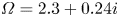. This behaviour is consistent with the observations from Zarzoso et al. (Reference Zarzoso, Sarazin, Garbet, Dumont, Strugarek, Abiteboul, Cartier-Michaud, Dif-Pradalier, Ghendrih and Grandgirard2013): the avalanche synchronises at the EGAM frequency when energetic particles are present.

Figure 2. Contour lines of $| D_G |$ for $q = 1.6$, $\tau = 1$ and $s = 1$ with 7 % energetic particles at 2.8 times the thermal velocity. Here $S = 0$. The EGAM frequency is $\varOmega = 2.47 + 0.07 i$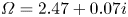. The zeros are in dark blue. The zeros arising from the zonostrophic instability are highlighted by red crosses.

The coupled instability develops at a resonance between the GAM frequency and the turbulent radial group velocity. The resonant radial wavenumber $k_r$ is a few times $s / q^2 \rho _i$. For weak magnetic shear, $k_r \rho _i$ is a fraction of a unit. The ordering assumption on the radial wavenumber is not ensured. Such inconsistency is typical of the wave-kinetic model (Parker Reference Parker2016). In addition, the quasi-linear framework, on which wave-kinetic theory is based, is known for its relevance well beyond its validity limits (Laval, Pesme & Adam Reference Laval, Pesme and Adam2018).

We emphasize that the unstable mode in figures 1 and 2 is not the GAM, but rather the zonostrophic mode which has been pushed-up by the GAM (although the converse can actually happen for EGAMs depending on the plasma parameters Girardo et al. Reference Girardo, Zarzoso, Dumont, Garbet, Sarazin and Sharapov2014). Furthermore, being a resonance process, the destabilisation by the GAM weakens when the GAM damping increases. For GAMs with a sufficiently high damping rate, this mechanism may not operate at all. Similarly, when the damping rate of the GAM depends on the radial position, the dynamics could select the most unstable growth rate for an enlarged radial span, and ensure an undamaged propagation through nonlinear effects. Therefore, we interpret the results from Villard et al. (Reference Villard, McMillan, Lanti, Ohana, Bottino, Biancalani, Novikau, Brunner, Sauter and Tronko2019) as a destabilisation of our unstable mode close to the edge, at the edge GAM frequency. This mode would propagate inwards from the edge, keeping this edge GAM frequency.

In contrast to the slab drift-wave problem, the unstable modes featured in the dispersion relation (6.19) have bounded growth rates, even for high wavenumbers. This can be shown easily by considering the limit of large growth rate as

(6.22)\begin{gather} D_G (\varOmega\rightarrow\infty) \approx \frac{1}{q^2} - \frac{J_2 (\varOmega)}{2}-\frac{1}{\varOmega^2 \tau + \varOmega^2 \frac{P^2}{q^2} - 1/2} \end{gather}

(6.23)\begin{gather}J_2 (\varOmega\rightarrow\infty) \approx \frac{2}{\varOmega^2} - \frac{8 P^2 / s}{\varOmega^2 - P^2 / s^2} \left[\mathcal{T}_c - \textrm{i} \frac{S}{\varOmega} \mathcal{T}_s \right]. \end{gather}

Solving this dispersion relation reduces to the roots of the following quartic equation

(6.24)\begin{equation} \varOmega^4 P^2 s^2 - \varOmega^2 \left(P^4 + P^2 q^2 s^2 + 4 P^4 q^2 \mathcal{T}_c + q^4 s^2\right) + P^4q^2 + P^2 q^4 = 0, \end{equation}

which has four real roots for $P$ that are sufficiently large. As a consequence, the approximation of static free-energy sources is acceptable, even in the thin-corrugation limit. This contrasts with the situation of slab drift-waves, where Parker (Reference Parker2016) found this approximation leads to unphysical results.

If we add a non-zero background zonal shear, we expect the system to develop an asymmetry depending on the sign of $\varOmega$. This is not the case without a turbulent growth rate. Turbulent structures are allowed to travel the full poloidal plane. The system is symmetric in phase velocity, and does not prefer a direction over another. This is a consequence of the joint symmetry principle (Hwa & Kardar Reference Hwa and Kardar1992; Diamond & Hahm Reference Diamond and Hahm1995). To regain the asymmetry, we need to take into account the differential growth between the two sides. The damping on the high-field side cuts the poloidal travel of the turbulent structures. We add a growth rate $\gamma = \alpha \cos \zeta$ to (6.1). The $\alpha$ coefficient constrains a localised growth of the turbulence on the low-field-side. This effectively expresses the intensity growth where the instability growth is maximum. The $J_2$ function becomes

(6.25)\begin{equation} J_2 = I_2 - \frac{P^2 / s}{\varOmega^2 + 2 A^2 - S^2 - P^2 / s^2} \left[\left( 1 - \frac{AS}{\varOmega P} \right) \mathcal{T}_c - \textrm{i} \left(\frac{S}{\varOmega} - \frac{A}{P} \right) \mathcal{T}_s \right], \end{equation}

where $A = \alpha / u_{ {\operatorname {TR}}}$. By introducing $A \neq 0$, the structures are damped when arriving at the high-field side. The symmetry between $\zeta > 0$ and $\zeta < 0$ is broken, and the instability can develop with a preferred direction. We consider this modified system with $A = S = 2$. The dispersion relation for $P = 3$ is shown in figure 3. The two instabilities are located at $\varOmega = - 2.3 + 0.41 i$ 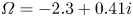and $\varOmega = 2.3 + 0.11 i$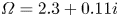. The direction is consistent with the observed inwards avalanches for positive zonal flow shear. In contrast to Sasaki et al. (Reference Sasaki, Itoh, Kobayashi, Kasuya, Fujisawa and Itoh2018a), we do not need to introduce an ad hoc up-down asymmetry of the turbulence spectrum, as it is generated self-consistently by the ballooned growth rate and the background flow shear. Nevertheless, such an asymmetry should be expected for tokamaks with realistic magnetic geometry, which would modify the directionality of avalanches as emphasised in Hager & Hallatschek (Reference Hager and Hallatschek2012). Although the wave–particle energy exchange is not self-consistent for $\alpha \neq 0$, the instability mechanism already exists in the self-consistent $\alpha = 0$ case. As a result, the computed instability is not spurious, but a modification of the former case.

Figure 3. Contour lines of $| D_G |$ for $q = 1.6$, $\tau = 1$ and $s = 1$. Here $A = S = 2$. The unstable inwards mode $\varOmega < 0$ is more unstable than the outwards mode. The $- 2 < \varOmega < 2$ region has been compressed to help visualisation in the $2 < | \varOmega | < 4$ regions.