


1. Introduction
Turbulence driven by cross-magnetic-field pressure gradients arises in a variety of natural (e.g. the Earth's magnetosphere) and laboratory (e.g. magnetically confined plasmas for fusion energy application) settings. For magnetized plasmas where the ratio of thermal energy density to magnetic energy density, $\beta$ , is low, the pressure-gradient-driven instabilities and the resulting turbulence is expected to be largely electrostatic (Liewer Reference Liewer1985; Carreras Reference Carreras1997; Doyle Reference Doyle2007) as field-line bending or compression is energetically unfavourable. As $\beta$
 is increased, these instabilities are expected to become more electromagnetic and this change is associated with important qualitative and quantitative changes in turbulence dynamics. First, unstable drift waves couple to Alfvén waves, which can substantially modify linear mode properties and the nature of the resulting turbulence (Jenko & Scott Reference Jenko and Scott1999). Second, the nonlinear saturation mechanisms can be affected, which modify the turbulence amplitudes and wavenumber spectra (Pueschel & Jenko Reference Pueschel and Jenko2010; Pueschel et al. Reference Pueschel, Hatch, Görler, Nevins, Jenko, Terry and Told2013; Whelan, Pueschel & Terry Reference Whelan, Pueschel and Terry2018). Third, inherently electromagnetic structures of the turbulence, like zonal fields or magnetic streamers, can develop at a wide range of $\beta$
 values (Smolyakov, Diamond & Kishimoto Reference Smolyakov, Diamond and Kishimoto2002). Fourth, the relative importance of electromagnetic transport processes with respect to electrostatic ones might increase with $\beta$
 as the electron heat flux along fluctuating magnetic field lines can carry a substantial part of the overall cross-field heat fluxes at high $\beta$
 (Rechester & Rosenbluth Reference Rechester and Rosenbluth1978; Weiland & Hirose Reference Weiland and Hirose1992; Pueschel, Kammerer & Jenko Reference Pueschel, Kammerer and Jenko2008). Fifth, new instabilities can develop as electromagnetic terms that were previously ignored become significant; for example, in tokamaks a transition from electrostatic instabilities, such as the ion temperature gradient, to electromagnetic instabilities, like the kinetic ballooning mode, as $\beta$
 is increased (Candy Reference Candy2005).
The study of turbulence and turbulent transport is critical to the development of viable magnetic confinement fusion devices. To maximize fusion power and access continuous operation via a large bootstrap fraction (Kikuchi Reference Kikuchi1993), fusion plasmas benefit from increased plasma $\beta$ (Citrin et al. Reference Citrin, Garcia, Görler, Jenko, Mantica, Told, Bourdelle, Hatch, Hogeweij and Johnson2015; Terry et al. Reference Terry, Carmody, Doerk, Guttenfelder, Hatch, Hegna, Ishizawa, Jenko, Nevins and Predebon2015). In finite $\beta$
 plasmas the role of magnetic fluctuations can become more important, as they can change the character of instabilities and the nature of the resulting anomalous transport (Rechester & Rosenbluth Reference Rechester and Rosenbluth1978; Weiland & Hirose Reference Weiland and Hirose1992; Candy Reference Candy2005). The mechanisms that lead to modified linear/nonlinear stability(Terry et al. Reference Terry, Li, Pueschel and Whelan2021), changes in turbulent flow generation and novel electromagnetic transport effects are still not fully understood (Lee et al. Reference Lee, Angus, Umansky and Krasheninnikov2015; Snyder & Hammett Reference Snyder and Hammett2001). Understanding pressure-gradient-driven turbulence in higher $\beta$
 plasmas is also of relevance to processes in near-Earth space including generation of coherent structures, energetic particle transport in the heliosphere and modification of magnetic reconnection in the presence of pressure gradients (Zimbardo et al. Reference Zimbardo, Perri, Pommois and Veltri2012; Pueschel et al. Reference Pueschel, Terry, Told and Jenko2015).
This paper reports on experiments in which the variation of pressure-gradient-driven turbulence is documented as a function of plasma $\beta$ . These experiments have been made possible through the use of a $\mathrm {LaB}_6$
 cathode plasma source in the Large Plasma Device (LAPD) (Gekelman et al. Reference Gekelman, Pribyl, Lucky, Drandell, Leneman, Maggs, Vincena, Van Compernolle, Tripathi and Morales2016). This source produces plasmas with up to a factor of 100 increase in plasma pressure compared with lower power density plasma sources, which, along with a lowered magnetic field, enable access to moderate $\beta$
 values (${\sim } 0.1\text {--}1$
 ) while maintaining ion magnetization. In these experiments, plasma $\beta$
 is varied from ${\approx } 0.2\,\%$
 up to ${\approx } 15\,\%$
 . From the scan, normalized density fluctuations are seen to decrease slightly with increasing $\beta$
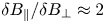
 while normalized magnetic fluctuations increase substantially, going from $\delta B/B_0 \sim 0.06\,\%$
 at the lowest $\beta$
 to $\delta B/B_0 \sim 1\,\%$
 at the highest $\beta$
 values. Importantly, parallel magnetic fluctuations represent a large fraction of the fluctuation amplitude; they are comparable in magnitude to perpendicular fluctuations at $\beta \sim 1\,\%$
 but are a factor of two larger at the highest $\beta$
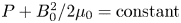
 . The magnitude of parallel magnetic fluctuations is consistent with the dynamic pressure balance in the turbulence: $P + {B_0}^2/(2\mu _0)= \textrm {constant}$
 . The measurements are compared with predictions from a simple slab model of resistive drift-Alfvén waves, extended to include compressive magnetic fluctuations and increased $\beta$
 .
.
2. Experimental set-up
The LAPD (Gekelman et al. Reference Gekelman, Pribyl, Lucky, Drandell, Leneman, Maggs, Vincena, Van Compernolle, Tripathi and Morales2016), shown schematically in figure 1, produces an 18 m long cylindrical magnetized plasma using emissive cathode discharges. Two plasma sources are used during these experiments. The primary LAPD cathode is a 75 cm BaO-coated nickel cathode that produces a 60 cm diameter background plasma with density $n \sim 10^{12}\ \textrm {cm}^{-3}$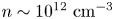 . A secondary plasma source has been installed on LAPD, which uses a smaller $\mathrm {LaB}_6$
 cathode that can produce higher-power-density discharges leading to a higher density plasma column (${\approx } 20\ \textrm {cm}$
 diameter) Gekelman et al. (Reference Gekelman, Pribyl, Lucky, Drandell, Leneman, Maggs, Vincena, Van Compernolle, Tripathi and Morales2016). The smaller LaB$_6$
 cathode is installed on the opposite end of LAPD, which allows for simultaneous operation with the primary BaO cathode. For the experiments reported in this paper, a helium plasma with a density of $2\times 10^{13}\ \mathrm {cm}^{-3}$
 and peak electron temperature of ${\sim }4\ \textrm {eV}$
 was produced by discharging the $\mathrm {LaB}_6$
 source in the afterglow of the primary BaO plasma source.

Figure 1. Schematic of the experimental set-up on the LAPD (not to scale). Staggered discharges of both cathode sources and a reduction of the background field in the middle of the device are used to reach a higher plasma $\beta$ than during normal operation.
Previous experiments in LAPD have investigated turbulence driven by pressure gradients and flow in the lower $\beta$ plasma produced by the BaO cathode. These studies have included: excitation of drift-Alfvén waves by filamentary structures (Morales et al. Reference Morales, Maggs, Burke and Pe nano1999; Burke, Maggs & Morales Reference Burke, Maggs and Morales2000; Pe nano, Morales & Maggs Reference Pe nano, Morales and Maggs2000; Pace et al. Reference Pace, Shi, Maggs, Morales and Carter2008), intermittent turbulence and turbulent structures (Carter Reference Carter2006; Pace et al. Reference Pace, Shi, Maggs, Morales and Carter2008; Maggs & Morales Reference Maggs and Morales2012), modification of turbulence and suppression of transport by sheared flow (Maggs, Carter & Taylor Reference Maggs, Carter and Taylor2007; Carter & Maggs Reference Carter and Maggs2009; Zhou et al. Reference Zhou, Heidbrink, Boehmer, McWilliams, Carter, Vincena, Friedman and Schaffner2012; Schaffner et al. Reference Schaffner, Carter, Rossi, Guice, Maggs, Vincena and Friedman2013), flow and shear-flow driven instabilities (Horton et al. Reference Horton, Perez, Carter and Bengtson2005, Reference Horton, Correa, Chagelishvili, Avsarkisov, Lominadze, Perez, Kim and Carter2009; Schaffner et al. Reference Schaffner, Carter, Rossi, Guice, Maggs, Vincena and Friedman2013), and avalanche transport events driven by pressure gradients (Van Compernolle & Morales Reference Van Compernolle and Morales2017).
The experiments reported here build on this previous work, and seek to document changes to pressure-gradient-driven turbulence and associated transport as a function of plasma $\beta$ . Increased plasma $\beta$
 is in part accessed through the higher pressure plasma produced by the LaB$_6$
 source. Additional control over plasma $\beta$
 is accomplished through varying the background magnetic field. In this study, the field was varied from 1000G to 175G, which resulted in a core plasma $\beta$
 range of 0.17–15 %, respectively. Diamagnetic modifications of the mean field were measured and, at the highest $\beta$
 , represented a $5\,\%$
 reduction in the applied background field. As the field strength was varied, Langmuir probe and line-averaged interferometer measurements confirmed that the peak plasma density did not change substantially. Using the field strength to vary plasma $\beta$
 has its drawbacks as other dimensionless parameters are not held fixed in the scan; in particular $\rho ^* = \rho _s/a$
 , where $\rho _s$
 is the ion sound gyroradius and $a$
 is the scale length in the plasma, here taken to be the plasma diameter. This parameter varied from $\rho ^* \sim 0.02$
 to $\rho ^* \sim 0.1$
 over the range of magnetic field used in this study.
Measurements of the electron density, electron temperature and potential (both plasma and floating potential) were made using Langmuir probes axially located in the centre of the machine. Mean electron density profiles were determined using ion saturation current ($I_\textrm {sat} \propto n \sqrt {T_e}$ ) measured by a fixed-bias double Langmuir probe and electron temperature determined from triple Langmuir and swept Langmuir probes. The mean density profile measurements were calibrated using line-averaged density measurements made by a microwave interferometer. Mean plasma potential profiles were determined from high-spatial-resolution floating potential measurements which were calibrated to the swept Langmuir probe measurements at specific radial locations. Plasma density and potential fluctuations were inferred from fluctuations in the ion saturation current and in the floating potential from a Langmuir probe; these signals were analysed assuming that temperature fluctuations were negligible to infer characteristics of the density and potential fluctuations. Measurements of magnetic field fluctuations were made with three-axis magnetic induction (or ‘B-dot’) probes (Everson et al. Reference Everson, Pribyl, Constantin, Zylstra, Schaeffer, Kugland and Niemann2009). Changes to the background magnetic field arising from diamagnetic effects were determined using time-integrated measurements of $\dot {B}_z$
 from the three-axis coils.
3. Experimental results
Figure 2 shows profiles of the mean plasma density and electron temperature for different values of core $\beta$ (different values of applied magnetic field). The core plasma density and steepness of the edge gradient are similar for all $\beta$
 values. Electron temperature grows significantly in width, as lowering $B_0$
 in the centre of the machine while holding $B_0$
 constant at the cathode sources to reach higher $\beta$
 causes flaring. A slight asymmetry in the profiles can be attributed to the perturbing nature of probe effects with a small target plasma. Diagnostics enter from the $r=30\ \textrm {cm}$
 side and must traverse the entire plasma column to measure the $r=-20\ \textrm {cm}$
 side of the dataset. Thus, subsequent analysis in this paper will focus on the right side of the column where $r>0\ \textrm {cm}$
 .
.

Figure 2. (a) Density and (b) electron temperature mean radial profile measurements for different values of core $\beta$ . Core density is similar for all $\beta$
 whereas electron temperature grows significantly in width as the background field in the centre of the machine is lowered to reach higher $\beta$
 .
.
A magnetic pick-up probe was used to measure the low-frequency variation of the background magnetic field arising from diamagnetism; time traces of the the reduction of the magnetic field in the core plasma at four different plasma $\beta$ conditions are shown in figure 3 with the reduction becoming more prominent with increasing $\beta$
 . By averaging the time traces from $t = 12$
 to $t = 15\ \textrm {ms}$
 , radial profiles of the background magnetic fields, including their diamagnetic reductions, at different $\beta$
 can represented as the magnetic pressure ($P_{\textrm {mag}} = {B_{0}^2}/{2\mu _0}$
 ) in figure 4. By also overlaying the plasma pressure ($P_{\textrm {plasma}} \approx n_et_e$
 ) and total pressure ($P_{\textrm {plasma}}+P_{\textrm {mag}}$
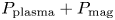 ) one can confirm that the radial pressure balance:

is satisfied to within $2\,\%$ .
.

Figure 3. Time traces of normalized diamagnetic reductions to the background field (solid line) and discharge current to the $\mathrm {LaB}_6$ cathode source (dashed line) at four different plasma $\beta$
 conditions: (a) 0.17 %; (b) 1.1 %; (c) 3.1 %; and (d) 8.4 %. Reduction increases with $\beta$
 .
.

Figure 4. Radial profiles of magnetic and plasma pressure (dashed) as well as the sum (solid) normalized to the maximum total pressure at four different plasma $\beta$ conditions: (a) 0.17 %; (b) 1.1 %; (c) 3.1 %; and (d) 8.4 %. Pressure balance holds (within 2 %) as the radial localizations of increases in plasma pressure are matched with the decreases in magnetic pressure.
The radial profiles of the mean plasma density along with the temporal root-mean-square (r.m.s.) density and magnetic field fluctuation amplitude for four different magnetic field values (four different core $\beta$ values) are shown in figure 5. These four $\beta$
 conditions are chosen for figure 5 to highlight key changes in the turbulence as the relative amplitudes among $\delta B_\parallel , \delta B_\perp$
 and $\delta n_e$
 change with $\beta$
 . Focusing first on the lowest $\beta$
 condition in figure 5(a), peaks in density fluctuations are observed that are localized to the maximum density gradient regions. Focusing on the magnetic fluctuation profiles, it is observed that the perpendicular fluctuations are localized to the core. After lowering the field to increase $\beta$
 modestly to 1.1 %, as seen in figure 5(b), these perpendicular magnetic fluctuations begin to grow and the appearance of parallel magnetic fluctuations localized to the edge pressure gradients are first observed.

Figure 5. Mean density radial profile and density/magnetic temporal r.m.s. fluctuation profiles at four different plasma $\beta$ conditions: (a) 0.17 %; (b) 1.1 %; (c) 3.1 %; and (d) 8.4 %. The $\delta B_\parallel$
 and $\delta n_e$
 fluctuations are localized to the gradient region while $\delta B_\perp$
 fluctuations are localized to the core for all $\beta$
 conditions.
The $\delta B_\parallel$ fluctuation spectra for $\beta = 1.1\,\%$
 , shown in figure 6, reveals that most of the power is concentrated at a low-frequency peak ($\omega \sim 0.003\omega _{\textrm {ci}}$
 where $\omega _{\textrm {ci}}$
 is the ion cyclotron frequency) with additional semicoherent peaks at higher frequencies. While not shown, the fluctuation spectra for $\delta n_e$
 and $\delta B_\perp$
 are also very similar to that of $\delta B_\parallel$
 and strongly correlated. This suggests that while the radial localization is different for some fluctuating quantities, these fluctuations are created by the same global mechanism.

Figure 6. Power spectra of $\delta B_\parallel$ fluctuations for many $\beta$
 conditions. Most of the power is located at low frequency while peaks at higher frequencies grow in power with increasing $\beta$
 until the emergence a single coherent peak at the highest $\beta$
 .
.
Core localization of perpendicular magnetic fluctuations is consistent with previous observations of low-$m$ drift-Alfvén waves in smaller plasma columns in LAPD (Burke et al. Reference Burke, Maggs and Morales2000). One can demonstrate that the observed fluctuations are low-$m$
 cylindrical eigenmodes by looking at the spectral two-dimensional (2-D) cross-correlation $C_{\textrm {spec}}$
 among the different magnetic directions at the low-frequency peaks seen in figure 6. This zero time-delay correlation function is computed in terms of an integral over the cross-spectrum between the time series of a stationary reference probe ($I_{\mathrm {ref}}$
 ) and an axially offset moving probe ($I_{\textrm {mov}}$
 ) for frequency bandwidths $[f-\delta ,f+ \delta ]$
 . The function is as follows:

whereby $C_{\textrm {spec}}(x, y, \omega )$ is normalized by $C_{\max }$
 for the 2-D plane, $\theta$
 is the spectral cross-phase between $I_{\mathrm {ref}}$
 and $I_{\textrm {mov}}$
 fluctuations, and $\gamma$
 is the coherency between the two signals. Frequency bandwidths are small ($\delta = 0.0012 \omega _{\textrm {ci}}$
 ) and $\omega$
 is chosen to isolate specific modes that display the clearest spatial structures.
Using this technique, for $\beta = 1.1\,\%$ it is observed in figure 7(a) that the $\delta B_\parallel$
 structure is localized to the gradient edge region of the plasma, consistent with an $m = 1$
 eigenmode and is coherent for higher frequency modes such as $m = 3$
 seen in figure 7(b). A slight discrepancy in the location of frequency peaks seen in figure 6 and the $\omega$
 selected in figure 7 arises from the fact that the data collected to produce each figure are from different runs where slight changes in the plasma are expected.

Figure 7. (a) Cross-spectral power between a moving $B_\parallel$ and stationary $n_e$
 probe at $\beta = 1.1\,\%$
 for (a) $\omega \approx 0.0024 \omega _{\textrm {ci}}$
 showing a coherent $m = 1$
 structure and (b) $\omega \approx 0.056 \omega _ci$
 showing an $m = 3$
 structure. The contour lines map out the density profile.
Figure 8(a) shows $B_\perp$ fluctuation power localized to the core of plasma while computing the parallel current $J_\parallel$
 shows distinct current channels localized on the density gradient. These observations are consistent with a low-$m$
 drift-Alfvén wave, as will be shown in more detail below. Similar cross-correlation data were taken at higher values of $\beta$
 and seen to be qualitatively equivalent.

Figure 8. (a) Cross-spectral power between a moving $B_\perp$ and stationary $n_e$
 probe at $\beta = 1.1\,\%$
 for $\omega \approx 0.0024 \omega _{\textrm {ci}}$
 with $B_x , B_y$
 vectors on top. Pattern matches the expected core localization for a drift-Alfvén wave. (b) Parallel current calculated from $\boldsymbol {\nabla } \times \boldsymbol {B}_\perp$
 that matches the expected current channels on the density gradient. The contour lines map out the density profile.
Continuing to increase $\beta$ , as seen in figure 5(c), the radial locations of the fluctuation peaks remain constant relative to the density profile. Focusing on the amplitude of the peaks, density fluctuations are seen to modestly decrease while both the parallel and perpendicular magnetic fluctuations increase with higher $\beta$
 . Of particular interest, at the highest $\beta$
 condition, as seen in figure 5(d), the relative magnitude of $B_\parallel$
 fluctuations exceeds that of $B_\perp$
 . This trend can be quantified by tracking the peak amplitude of the different types of fluctuations for additional intermediate plasma $\beta$
 conditions. As shown in figure 9(a), this analysis demonstrates that both parallel and perpendicular fluctuations increase rapidly with increasing $\beta$
 until they diverge from one another at $\beta \sim 2\,\%$
 . For $\beta > 2\,\%$
 the peak parallel fluctuation level continues to increase, albeit at a slower rate, while perpendicular fluctuations saturate and remain mostly constant until reaching the highest $\beta > 10\,\%$
 conditions of the data set. Figure 9(b) quantifies this trend by analysing the ratio of parallel to perpendicular magnetic r.m.s. (temporal) fluctuation levels. This ratio is shown to grow beyond order unity for $\beta \geq 2\,\%$
 and reach a factor of 2 at the highest $\beta$
 .
.

Figure 9. (a) Peak r.m.s. fluctuation levels for magnetics and density as a function of plasma $\beta$ . Here $\delta B_{\parallel },\delta B_{\perp }$
 grow with $\beta$
 while $\delta n_e$
 decreases. (b) Ratio of parallel to perpendicular magnetic peak r.m.s. fluctuation power which also increases past order unity for $\beta \geq 2\,\%$
 .
.
Characterizing this unique growth of $B_\parallel$ fluctuations, the changes in fluctuation spectra at different $\beta$
 conditions are analysed. Figure 6 shows how low-frequency fluctuations are dominant for all $\beta$
 conditions. At the lower $\beta$
 there are multiple higher frequency peaks which correspond to the higher $m$
 -number mode structures such as the $m = 3$
 seen in figure 7(b). As $\beta$
 increases, these multiple higher frequency peaks disappear and a single coherent peak at ${\approx } 0.02 \ \omega _{\textrm {ci}}$
 arises.
One physical mechanism for the generation of parallel magnetic field perturbations is the perturbed diamagnetic currents that arise owing to density fluctuations in an increased $\beta$ plasma. This mechanism is equivalent to the dynamic pressure balance between the magnetic and plasma pressure fluctuations. From (3.1), the pressure balance can be written for the fluctuation quantities as

such that

From (3.3) it is predicted that $B_\parallel$ and $\delta P$
 fluctuations should be out of phase by ${\rm \pi}$
 radians with one another and that the left-hand and right-hand sides should be of the same order of magnitude. Figure 10 confirms this with $\delta P /(B_{0}^2/\mu _0)$
 and $\delta B_{\parallel } / B_{0}$
 having the correct sign and having a fairly good linear fit to the predicted $1:1$
 relationship.

Figure 10. Pressure balance, $\delta P ({B_0}^2/\mu _0)$ versus $\delta B_{\parallel } / B_0$
 for different $\beta$
 conditions. Dotted line represents the expected result for pressure balance, which is qualitatively consistent and follows the correct trend for different $\beta$
 .
.
The prediction in (3.4) can be further validated by looking at cross-correlation functions between $\delta B_\parallel$ and $\delta n_e$
 fluctuations. Figure 11(a) shows the same spectral band passed cross-correlation function, $C_{\textrm {spec}}$
 , from figure 7 between two $n_e$
 probes located 5 m apart in the axial direction at $\beta = 1.1\,\%$
 . One probe is stationary on the density gradient at $r=10\ \textrm {cm}$
 while the other traverses the plasma column in the $XY$
 plane and the signals are correlated to one another using the same technique as (3.2).

Figure 11. Strong anti-correlation at $\beta = 1.1\,\%$ of $\delta n_e$
 and $\delta B_\parallel$
 fluctuations by showing (a) cross-correlation between a moving $n_e$
 and stationary $n_e$
 probe with (b) correlation between a moving $B_\parallel$
 and the same stationary $n_e$
 probe with the dotted circle indicating the location of maximum correlation from (a). The contour lines map out the density profile.
The area outlined by the black dotted line indicates the location of the stationary probe $(x_{\mathrm {ref}},y_{\mathrm {ref}})$ as it is the location of highest correlation. Figure 11(b) uses the same stationary probe as figure 11(a) but is instead correlated to a moving $B_\parallel$
 probe located 5.5 m away axially. As seen from the outlined circle, which represents the position of the stationary $n_e$
 probe, the fluctuations between $B_\parallel$
 and $n_e$
 appear to be highly anti-correlated. This is consistent with the theory of pressure balance.
One can now compute $C_{\textrm {spec}}(x_{\mathrm {ref}},y_{\mathrm {ref}},\omega )$ at the location of the stationary $n_e$
 probe for a larger frequency range. Doing so allows for the individual contributions, such as the coherence $\gamma$
 and phase difference $\theta$
 between $B_\parallel$
 and $n_e$
 fluctuations, at all frequencies to be quantified. As seen in figure 12(a), there are a few semicoherent peaks on top of a broadband spectrum which primarily arise from the corresponding peaks in cross-coherence between the two signals, as seen in figure 12(b). From figure 12(c) it is observed that for all low frequencies the cross-phase between $n_e$
 and $B_\parallel$
 is ${\rm \pi}$
 radians out of phase.

Figure 12. (a) Cross-correlation ($C_{\textrm {spec}}(x_{\mathrm {ref}},y_{\mathrm {ref}},\omega )$ ), (b) cross-coherence ($\gamma$
 ) and (c) cross-phase ($\theta$
 ) between $\delta n_e$
 and $\delta B_{\parallel }$
 at $\beta = 1.1\,\%$
 . For all $\omega < 0.1 \omega _{\textrm {ci}}$
 the mode has a coherent ${{\rm \pi} }/{2}$
 phase difference.
Investigating further, a decomposition of the polarization of the wave to be either right-handed (rotating in the electron direction) or left-handed (rotating in the ion direction) can be made. This technique involves summing together Fourier transforms of $B_x$ and $B_y$
 core fluctuations in frequency space and adding phase differences of $+{{\rm \pi} }/{2}$
 (right-handed) or $-{{\rm \pi} }/{2}$
 (left-handed) (Terasawa et al. Reference Terasawa, Hoshino, Sakai and Hada1986; Weidl et al. Reference Weidl, Winske, Jenko and Niemann2016) as follows:


where $\widetilde {B_x}(\omega )$ is the Fourier transform of $B_x$
 . Then $\widetilde {B_{L,R}}(\omega )$
 are transformed back to the time domain and, by analysing the power of the r.m.s. fluctuations in each case, one can determine whether the instability is primarily right- or left-handed by defining percent power as

Repeating this analysis for many $\beta$ conditions, as seen in figure 13, it is concluded that the wave is predominantly left-handed for low-$\beta$
 conditions. However, as $\beta$
 increases, there is a distinct shift where the turbulence changes to become more right-handed in nature. Because drift-Alfvén waves are typically left-hand polarized, this analysis further points to the turbulence being caused by a modified drift-Alfvén for the majority of $\beta$
 conditions studied in this experiment. The deviation to right-hand polarization at the higher $\beta$
 conditions could indicate a new instability developing and explain the multiple higher frequency peaks coalescing around a single peak for $\beta > 10\,\%$
 , as seen in figure 6.

Figure 13. Power-weighted handedness of $\delta B_{\perp }$ fluctuations at various $\beta$
 conditions. Instability changes from left-handed to right-handed dominant with increasing $\beta$
 .
.
4. Discussion
Initial observations led to a proposal that the data could be the result of a new instability, the gradient-driven drift coupling mode or GDC instability (Pueschel et al. Reference Pueschel, Jenko, Told and Büchner2011, Reference Pueschel, Terry, Told and Jenko2015, Reference Pueschel, Rossi, Told, Terry, Jenko and Carter2017). The GDC was originally observed in kinetic simulations of magnetic reconnection and had characteristics similar to those observed in the LAPD data, in particular, correlated density and parallel magnetic field fluctuations with the magnetic field fluctuations out of phase with the density fluctuations. Kinetic simulations with LAPD pressure profiles and parameters indicated growth of the GDC in plasmas relevant to these experiments (Whelan et al. Reference Whelan, Pueschel and Terry2018). However, it was pointed out that the simulations that gave rise to the GDC as a new instability were run in out-of-equilibrium conditions, with pressure gradients but not including the gradients in the background magnetic field that should arise in the pressure balance in finite $\beta$ plasmas and are observed in this dataset. An exact force balance causes the GDC to become linearly marginally stable (Rogers, Zhu & Francisquez Reference Rogers, Zhu and Francisquez2018). In addition, the GDC simulations do not predict correlated perpendicular magnetic fluctuations, as observed in the experimental data. Recent simulations of the GDC in electron–positron plasmas indicate that the GDC can nonlinearly persist in plasmas where a radial pressure balance exists (where gradients in the background field develop) (Pueschel et al. Reference Pueschel, Sydora, Terry, Tyburska-Pueschel, Francisquez, Jenko and Zhu2020) and as such we do not rule out the possibility that the GDC could play a role in the saturated turbulent state that is observed in the experiments.
Nonetheless, given the similarity of the observed fluctuations in low-$\beta$ conditions to drift-Alfvén waves, it would be remiss to not pursue whether the observed modes are modified drift-Alfvén waves. At lower $\beta$
 , the characteristics of the observed fluctuations are consistent with previous observations of low-$m$
 drift-Alfvén waves in LAPD. In particular, the mode pattern of correlated perpendicular magnetic and density fluctuations and the polarization of the perpendicular magnetic fluctuations are fully consistent. As $\beta$
 is increased, parallel magnetic fluctuations grow, correlated with the perpendicular magnetic and density fluctuations. This observation is not consistent with the standard picture of the drift-Alfvén wave and motivates the following investigation of a modified drift-Alfvén wave theory.
A local, slab-model linear theory has been developed, starting from a Hall–MHD derivation of drift-Alfvén waves outlined by Goldston (Goldston & Rutherford Reference Goldston and Rutherford1995). Additional terms were added to include fluctuations in the background magnetic field and including the non-uniform background field that arises from diamagnetic effects at increased plasma $\beta$ . The ordering of additional terms was determined by using experimental measurements of the amplitude of fluctuating quantities. The resulting linear model is detailed in Appendix A.
Growth rates and instability characteristics of this model were computed using experimentally measured profiles for the lowest $\beta$ condition and assuming $\lambda _\parallel = 2L_\parallel$
 (where $L_\parallel$
 is the axial length of the machine). By then decreasing $B_0$
 , one can perform a scan in plasma $\beta$
 . As shown in figure 14, for all values of $\beta$
 there appeared to be an unstable mode and the growth rate increased with $\beta$
 .
.

Figure 14. Growth rate of fastest growing mode from local theory at various $\beta$ conditions.
In addition, this local theory can be used to compute ratios of amplitudes and phase differences for various fluctuating quantities to compare with experimental results. As detailed in Appendix A, the amplitude ratio between $\delta B_\parallel$ and $\delta n$
 can be derived as follows:

Figure 15 shows this ratio computed, using experimentally measured profiles and the $\omega$ and $k_\perp$
 of the fastest growing mode for each $\beta$
 , along with experimental measurements. There is relatively good agreement between the linear theory prediction and experimental measurement for $\beta < 2\,\%$
 with deviations at the higher $\beta$
 . The ratio between $\delta B_\parallel$
 and $\delta B_\perp$
 can also be computed from the model (see Appendix A):


Figure 15. Ratio of parallel magnetic to density fluctuation amplitude as a function of $\beta$ .
.
By performing a comparison of the theoretical predictions to experimental results, as seen in figure 16, the ratio of these fluctuations increased with $\beta$ in a similar fashion to the experimental results for $\beta < 2\,\%$
 . While the parallel wavelength of the mode was not able to be measured directly, the theoretical predictions suggest that $\lambda _{\|}$
 is many machine lengths, as seen by the improved agreement for larger $\lambda _{\|}$
 .
.

Figure 16. Ratio of parallel to perpendicular magnetic fluctuation amplitude for experimental data and using a theoretical model with different values of $\lambda _{\parallel }$ , where $L_{\parallel }$
 is the axial length of the machine. The ratio is seen to generally increase with increasing $\beta$
 with the best agreement between theory and experiment at higher $\lambda _{\parallel }$
 .
.
While the experimental data are consistent with the predictions of the slab-based local model at lower $\beta$ , the agreement begins to break down at $\beta > 2\,\%$
 . This could be explained by finite Larmor radius (FLR) effects becoming important as lowering the background magnetic field to increase $\beta$
 also increases the ion gyroradius such that only a few ion gyroradii fit within the pressure gradients of the experiment. Future work will seek to address this through the development of a global kinetic model that includes significant $\delta B_\parallel$
 fluctuations to capture more of the physics involved with the predominantly low-$m$
 modes observed.
5. Conclusions
In this experiment, the variation of pressure-gradient-driven turbulence and transport for increased $\beta$ (up to $\beta \approx 15\,\%$
 ) is documented in a linear, magnetized plasma. Magnetic fluctuations are observed to grow with increasing beta. A novel result is that parallel magnetic fluctuations are dominant at higher $\beta$
 , increasing up to $\delta B_\parallel / \delta B_\perp \approx 2$
 with $\delta B / B_0 \approx 1\,\%$
 . Parallel magnetic fluctuations are also strongly correlated with density fluctuations, which are observed to be out of phase with one another. Further analysis of fluctuation amplitude ratios between $\delta n_e$
 and $\delta B_\parallel$
 shows consistency with a dynamic pressure balance ($P+{B_{0}^2}/{2\mu _0} = \textrm {constant}$
 ). Consistency of the measured mode pattern with previous observations of drift-Alfvén waves motivates the derivation of a local slab-model theory for electromagnetic, modified drift Alfvén waves that includes parallel magnetic fluctuations and diamagnetic corrections to the background field. Comparison of turbulence characteristics between this theoretical model and experimental data shows promising agreement for $\beta <2\,\%$
 while differences at higher $\beta$
 prompts the need for future work in developing a global kinetic model to illuminate whether the differences are the result of a new instability or further modifications to a drift-Alfvén wave.
Acknowledgements
The authors thank Z. Lucky, M. Drandell and P. Pribyl for technical support in executing the experiments.
Editor Cary Forest thanks the referees for their advice in evaluating this article.
Funding
This work was performed using the Basic Plasma Science Facility, which is supported by US DOE and NSF. Support for this work came from DOE awards DE-FC02-07ER54918:0023, DE-SC0014113:0003; and from NSF award PHY-1561912:004.
Declaration of interests
The authors report no conflict of interest.
Appendix A
To derive a dispersion relation for electromagnetically modified drift waves, we follow Goldston's (Reference Goldston and Rutherford1995) analysis but carry through terms involving $\delta B_{\parallel }$ fluctuations and diamagnetic responses to the background field $\partial _x B_0$
 that would normally be neglected.
This derivation assumes a slab model plasma with a non-uniform density $n(x)$ whereby equilibrium is maintained by a strong background magnetic field, $B_0$
 . The plasma is also assumed to be at rest in the lab frame ($\boldsymbol {u}=0$
 ) but with a non-zero current density $J_y(x)$
 which provides the $\boldsymbol {J} \times \boldsymbol {B}$
 force to balance $\boldsymbol {\nabla } P$
 .
.
Starting with the perturbed equation of motion:

one uses Ohm's law to expand the $\hat {x}$ component to become

where $v_A^2 = {B_0^2}/{\mu _0 \rho _0}$ is the Alfvén speed and $k_\perp ^2 = k_x^2+k_y^2$
 . To now link $\delta u_x$
 , $\delta B_x$
 and $\delta B_\parallel$
 , one can combine Faraday's law (${ \partial _t \delta B_\parallel } = -\boldsymbol {\nabla } \times \delta \boldsymbol {E}$
 ) and Ampere's law ($\boldsymbol {\nabla } \times \boldsymbol {B} = \mu _0\boldsymbol {J}$
 ) with Ohm's law for first-order perturbed quantities ($\delta \boldsymbol {E} + \delta \boldsymbol {u} \times \boldsymbol {B} = \eta \delta \boldsymbol {J} + ({1}/{{ne}})\delta [\boldsymbol {J}\times \boldsymbol {B} - \boldsymbol {\nabla } {P_e}]$
 where $\eta$
 is resistivity) to obtain

where it is assumed $\omega \ll \omega _{\textrm {ci}}$ . If one also assumes that $T_e$
 is uniform along the field lines ($\boldsymbol {B} \boldsymbol {\cdot } \boldsymbol {\nabla } T_e = 0$
 ) but can have a gradient across the field, one can use this in conjunction with the continuity equation ($\partial _t n + \boldsymbol {\nabla } \boldsymbol {\cdot } n \boldsymbol {u} = 0$
 ) to rewrite the $\hat {z}$
 component of (A1) as

where $c_s = \sqrt {{T_e}/{M}}$ is the plasma sound speed. Now substituting (A4) into (A3) results in

where $v_{de}=({T_{e}}/{n_{e}e B_{0}})\partial _{x}n_{e}$ . One can now determine an expression for $\delta u_x$
 by rearranging (A2) to obtain:

If one now assumes pressure balance ($P+{B_{0}^2}/{2\mu _0} =$ constant) and negligible temperature gradients ($\partial _x T_e = 0$
 ) the first and second derivatives from (A6) can be rewritten using the substitutions

and

By now combining (A6), (A7) and (A8), and substituting into (A5), one can obtain the final dispersion relation:

Equation (A9) is similar to the dispersion relation found in Goldston's original derivation with two distinct branches, one for the shear Alfvén wave (a) and one for the Drift wave (b). However, by assuming non-zero values of $\beta$ we introduce a new secondary coupling term (c) as well as modify the second term in the shear Alfvén wave (a) part of the dispersion relation.
The derivation of this dispersion relation is not yet complete as the fluctuating quantities $\delta B_{\parallel }$ and $\delta B_{x}$
 are also functions of $\omega$
 and $k_\perp$
 . To determine this relationship one can start with the MHD equation of motion linearized to first order,

If one assumes that the zeroth-order $\boldsymbol {J}$ arises from the zeroth-order diamagnetic drift $u_d \approx \boldsymbol {\nabla } P \times \boldsymbol {B}$
 and the pressure profile $P(x)$
 only varies in the $x$
 direction and the zeroth-order $\boldsymbol {B}$
 is $B_\parallel$
 which points in the $z$
 direction, this means $\boldsymbol {J}$
 only points in the $y$
 direction. The $\hat {x}$
 component of (A10) can thus be written as

Now using Ampere's law ($\boldsymbol {\nabla } \times [\boldsymbol {B + \delta B}] = \mu _0 [\boldsymbol {J+\delta J}$ ]) for both zeroth and first order one can rewrite (A11) and combine it with (A6) to arrive at

Now by expanding $\partial _x \delta P_e$ and combining with (A4) and (A6), one can group the $\delta B_x$
 and $\delta B_\parallel$
 terms to arrive at the relation:

which can be substituted into (A9) to obtain a final dispersion relation explicitly in terms of $\omega$ and $k$
 .
.
Using the same assumptions a relation between $\delta n_e$ and $\delta B_\parallel$
 can be derived by taking (A12) to obtain:

Choosing to ignore the right-hand side and expand out terms to group the $\delta B_\parallel$ and $\delta n_e$
 terms one then arrives at

Because the ratio is more important than the additive offset, one can ignore the second term on the right-hand side and rearrange such that

and multiplying by the complex conjugate will yield

Using the algebraic expressions for the gradients:


and substituting into (A17) yields

which can now be rearranged to yield the normalized fluctuation amplitude ratio in terms of $\beta$ :
:


