1. Introduction
In the face of demographic ageing, numerous countries have implemented policies whose main target is to increase labor market participation and delay retirement. For example, numerous European countries have over the last several years implemented reforms increasing the full retirement age from 65 to 67 or beyond (OECD, 2015). Numerous countries have further reformed their legislation and/or changed implementing regulations in order to decrease demand for early exits, and this both from the labor demand and the labor supply side. On the demand side, this has sometimes translated into tighter conditions regarding company-level old-age layoff criteria, but also into larger financial contributions to the cost of early retirement schemes.Footnote 1 On the supply side, numerous measures have been taken to tighten conditions that individuals have to fulfill in order to access (early-) retirement benefits, and the generosity of some types of benefits has been decreased (if not discontinued altogether).
The paper contributes to the rich literature on supply-side factors, as surveyed in Coile (Reference Coile2015). With their widely cited study of a dozen developed countries, Gruber and Wise (Reference Gruber and Wise1999) no doubt provided a first large-scale investigation of labor supply factors. The work highlighted a strong positive correlation between (financial) retirement incentives and labor exits across their panel of countries. Blöndal and Scarpetta (Reference Blöndal and Scarpetta1999) and Duval (Reference Duval2003) have obtained similar results in cross-country studies. In a follow-up work, the various contributors to Gruber and Wise (Reference Gruber, Wise, Gruber and Wise2004) studied the econometric link between individual-level retirement incentives and labor supply. Using an option value specification à la Stock and Wise (Reference Stock and Wise1990), they found a strong empirical link between dynamic retirement incentives and labor market behavior: stronger marginal rewards to work lead to later retirement. This positive influence of the marginal reward to work on the retirement age is perfectly consistent with the idea of a substitution effect when price of early retirement increases. In the same way, higher levels of pension and social security wealth (SSW) should be expected to lead to higher probabilities of retirement in line with an income or wealth effect, at least insofar as leisure under the form of retirement is a normal good. However, and in stark contrast with this expectation, Gruber and Wise (Reference Gruber, Wise, Gruber and Wise2004) reveal wrong-signed income/wealth effects for numerous countries in their econometric work.
A second somewhat surprising finding of Gruber and Wise (Reference Gruber, Wise, Gruber and Wise2004) is that there is sometimes a large disparity between the sexes in the way incentives impact retirement decisions (e.g., Brugiavini and Peracchi, Reference Brugiavini, Peracchi, Gruber and Wise2004; Kapteyn and de Vos, Reference Kapteyn, de Vos, Gruber and Wise2004). Belloni and Alessie (Reference Belloni and Alessie2013), van Soest et al. (Reference van Soest, Kapteyn and Zissimopoulos2007) and Michaud and Vermeulen (Reference Michaud and Vermeulen2011) have all addressed this question in some way, and pointed the need to take the potential age and sex specificity of the parameters into account when modeling retirement decisions.
The structural retirement model of Stock and Wise (Reference Stock and Wise1990) – while providing a strong analytical background for retirement modeling but steering clear from the burdens of a full dynamic programming approach – also has some limitations and constraints. For example, Belloni and Alessie (Reference Belloni and Alessie2013) propose an extension of the basic structural model to include a random marginal value of leisure. We propose another methodological extension, namely a reduced-form variant of the Stock and Wise (Reference Stock and Wise1990) approach to introduce the household size into the model – an area so far under-explored. More specifically, our main contribution is a modification of the option value model to explicitly recognize differences between singles and couples both in their income streams and their retirement incentives.
On the empirical front, we apply our reduced form retirement model to recent Belgian data from the Survey on Health, Ageing and Retirement in Europe (SHARE). Belgium is a particularly interesting case study as it has a rich set of dependent and spousal benefits not only for the pension system itself, but also for several early retirement benefits (such as unemployment and disability insurance benefits). We provide results of the classical option value approach and of our augmented ones. This allows us to compare our results with previous estimations obtained for Belgium. The initial estimates of Dellis et al. (Reference Dellis, Desmet, Jousten, Perelman, Gruber and Wise2004) used administrative data from the period 1989–1996 – a time where Belgium displayed employment rates that were at their historical lows for men and upward trending for women of ages 50–59. Their results were fully in line with the general trends observed by Gruber and Wise (Reference Gruber, Wise, Gruber and Wise2004) for the wider set of countries. Later work by Jousten and Lefebvre (Reference Jousten and Lefebvre2013) as well as Jousten et al. (Reference Jousten, Lefebvre, Perelman and Wise2016) relied slightly different methodologies to derive retirement incentives and used more recent survey data (SHARE) instead of administrative information. The paper's main point of interest is whether the modified specifications improve results in a country like Belgium with its strong spousal/dependent benefit component.
The paper is structured as follows. The following section gives an overview of the Belgian retirement landscape and summarizes the Belgian SHARE data. Section 3 outlines our methodological improvements to the option value model and provides various summary statistics for various indicators of retirement incentives. Section 4 contains the empirical analysis of retirement decisions. Finally, Section 5 concludes.
2. Belgian retirement landscape and data
2.1. Employment in BelgiumFootnote 2
The Belgian labor market has undergone profound changes over the last decades. Figures 1 and 2 summarize employment rates for three older age groups since the beginning of standardized labor-market recordings through the Labor Force Survey in 1983. Since the 1980s and until the mid 1990s, male old-age employment displayed a sharp downward trend. For women, the situation was somewhat different, partly as a result of generally lower (but increasing) labor market attachment for women of all age cohorts, and partly as a result of a lower full retirement age for women (60) that has only gradually been aligned to the one for men (65) over the course of the period 1997–2009.

Figure 1. Men's employment rate, ages 50–54 to 60–64. Source: EU-LFS.

Figure 2. Women's employment rate, ages 50–54 to 60–64. Source: EU-LFS.
Still, employment rates remain low by international standards. Figures 3 and 4 plot the changes in employment rate for the population aged 50–64 for a selection of countries. They show that while there has been some catching-up Belgium still remains, in most years, sub-par as compared with its main economic partners, and this both for men and women.

Figure 3. International comparison men's employment rate, ages 50–64. Source: EU-LFS.

Figure 4. International comparison women's employment rate, ages 50–64. Source: EU-LFS.
2.2. Retirement and early retirement programs
What are the reasons for this poor labor market performance? Some of the answers can be found in the architecture of the Belgian social insurance schemes.
The Belgian social protection landscape can be grouped into three main schemes: the scheme for contractual wage-earners, the scheme for the self-employed and the scheme for civil servants. In what follows, we focus on the first one of these: the scheme for wage-earners which is the largest both in terms of current enrollment and in terms of its beneficiary population. The wage-earner scheme represents 49% of all retirees while the civil servant and the self-employed include 18% and 7% of the retirees respectively.Footnote 3 In terms of generosity, it can be positioned in between the somewhat less generous scheme for the self-employed and the overall more generous scheme for civil servants. Each scheme proposes coverage against a set of risks. For our purposes, we focus on insurance programs that have a special relevance for the early-retirement decision. In this context, the wage-earner scheme offers the full set of unemployment, (early-) retirement, and sickness and disability benefits, while the self-employed and civil servant schemes do not provide some covers (such as, e.g., unemployment insurance – though for different reasons for the two schemes).Footnote 4
The four main components of the wage-earner scheme of interest to the retirement decision are the unemployment, the early retirement, the sickness and disability and the pension insurance systems.Footnote 5 In the present section, we described the system as it was applicable during the period 2004–2009, which corresponds to the relevant timespan during which the SHARE waves 1 to 3 were collected (see below).Footnote 6
First, unemployment benefits were (and still are) not time limited in Belgium. During our period of study, two types of unemployment benefits were available to older workers: regular unemployment benefits and old-age unemployment benefits. The two key differences between both types of benefits reside in (i) that regular unemployed have to remain available for the job market and look for a job while old-age unemployed enjoy a sparing provision, and (ii) old-age unemployed enjoyed higher benefits. Since 2004, conditions for access to both provision has been tightened (starting in 2004 with a minimum of 20 years of qualifying career for the old-age supplement and a minimum age 58 for the job search waiver).
Though unemployment benefits have undergone a steady flow of reforms, some overarching features have remained intact and can be highlighted: First, regular and old-age unemployment benefits are a function of career length, unemployment duration and household status. During a first phase, unemployed with dependents reach a replacement rate of 60%, single unemployed 55% and cohabitants 40% of their last gross wage. Similarly, minimum and maximum unemployment benefits vary by household status and are decreasing in unemployment duration – with progressively stronger decreases for unemployed with dependents, singles and cohabitants.Footnote 7 Maximum and minimum old-age unemployment benefits display a similar conceptual structure – with increasing age further entering the picture as a third and attenuating dimension. Implicitly, Belgium thus has a single-earner supplement, though it is formally organized by means of a reduced duration-dependent generosity.
Second, early retirement programs have also been available to numerous older Belgian workers. Eligibility has been a function of age, career length and of the industry or company of employment. Access to the regular early retirement was set at 58 until 2007 and reached 60 as of 2008 until 2011. Career requirements have also simultaneously been tightened from 20 to 30 years. Earlier exits with lower career requirements were (and are) still possible for companies in restructuring or difficulties. Early retirement benefits consist of (i) a special unemployment insurance benefit corresponding to a replacement rate of 60% of the last gross wage and (ii) a top-up payment from the former employer (generally corresponding to half of the difference between the previous wage and the unemployment benefit). Contrary to regular or old-age unemployment benefits, the special early retirement unemployment benefits are neither dependent on the family situation nor duration dependent. Over most of the period of study, the normal access age was of 58 and was only raised to 60 as of 2008.
Third, sickness and disability benefits may also serve as early retirement pathways as described in Jousten et al. (Reference Jousten, Lefebvre, Perelman and Wise2012) and Jousten et al. (Reference Jousten, Lefebvre, Perelman and Wise2016). Sickness benefits are payable for the first 12 months of a sickness spell, period after which the individual will be rolled over into the disability insurance system. Sickness benefits rely on a complicated multi-stage process, with a first period covered by former employer (1 month for white collar workers, 14 days for blue collar workers), the second period up to and including the 12th month covered by the health insurance fund (with funds originating in the public social security system), and the third and final period of disability is covered by the social security system.
Regarding sickness and disability benefits, family status intervenes at two stages. Intriguingly, while sickness benefits are not household-status-dependent until month 6, the picture changes in month 7 where minimum and maximum sickness (and later disability) benefits start to take the household composition into account – through progressively lower benefits for singles and cohabitants as compared with those with dependents. Also more explicitly, the regular replacement rate for disability benefits is modulated as a function of the household type: 65% for people with dependents, 55% for singles, and 40% for cohabitants.
Last, but not least, regular retirement benefits provide for two main types of benefits: old-age and survivor benefits. Eligibility conditions have differed for men and women over the period of observation. For men, the key elements have been the following: a complete career consists of 45 years, the full retirement age is set at 65 and early retirement is possible as early as 60 without any actuarial adjustment if a career condition of 35 years is met. The full retirement age is particularly important insofar as it corresponds to the age that people on other social insurance benefits are automatically rolled over into the regular retirement system. For women, the period of observation corresponds to a transition phase where the full retirement age and the full career conditions were progressively adjusted upwards from their historical levels of 60° and 40 to 65 and 45 respectively – to align them to those applicable to men. More specifically, the full retirement age was of 63 in 2004–2005, 64 in 2006–2008 and 65 in 2009. The early retirement age has remained unchanged at age 60 during the full period of observation. Similarly, the early retirement career condition was satisfied with a career length of 34 years in 2004 and 35 years in 2005 and later.
Old-age retirement benefits offer a replacement rate to average indexed career earnings of 60% for singles or 75% for a retiree with a dependent spouse.Footnote 8 This 25% increase in the replacement rate for a retiree with a dependent spouse is thus economically equivalent to a ‘spousal benefit’ payable to the primary earner. In case the spouse has a pension entitlement of her own that is smaller the spousal benefit, then this own pension entitlement is dropped and the spousal supplement is payable to the primary earner. If the own entitlement is larger than the spousal benefit, the latter one is dropped.Footnote 9
Survivor benefits were available to surviving spouses of workers insofar as the survivor was aged more than 45. The benefit level of the survivor pensions corresponds to the level of the single retiree pension and can be combined with a person's own retirement pension up to an amount of 110% of the survivor pension.
2.3. SHARE data
In this paper we present new estimations of the effect of social security incentives on labor supply using data for Belgium collected by the SHARE. It is a cross-national panel database of micro data on health, socio-economic status, and social and family networks of European individuals aged 50 and more. It covers a broad range of variables of interest for employment and retirement analysis. Beyond more classical labor market data, the SHARE data has two distinct advantages as compared with other datasets available in Belgium: in contrast to the European Labor Force Survey (EU-LFS) or the European Survey on income and Living Conditions (EU-SILC) it contains detailed information on health status and work histories of the respondent and his or her partner; contrary to Belgian administrative data, it contains information on education level – though the latter comes at the cost of a loss of precision in terms of the richness and the sample size of administrative data.
We use SHARE data for Belgium that were collected between in 2004/2005, 2006/2007, and 2008/2009. While the first two waves mostly collect information on current situation of individuals, wave 3 (a.k.a. SHARELIFE) mostly targets life-cycle information, most notably work career data. We pool individuals from waves 1 and 2 and limit the sample to initially active individuals for whom we can reconstruct a lifetime earnings profile using information from SHARELIFE. More specifically, SHARELIFE contains information on current earnings, the start and end date of each past job, as well as the starting salary for each such job. We use this information to re-construct the earnings history of the individual over the entire life-cycle from the labor market entry until the year of interview – using linear interpolation in case of missing values. We then calculate the various hypothetical entitlements of individuals associated with each exit route.
The variable Age is defined as the age of the individual at the moment of the survey, taking into account his or her month of birth as compared with the month (s)he was surveyed. An individual is considered to be employed whenever (s)he self-reports being in gainful employment at the moment of the survey. We use the specific questions provided in SHARE that allow us to classify respondents’ employment status and identify whether (s)he is a wage earner, self-employed or civil servant.Footnote 10 Exit from the labor market is obtained by looking at the status declared in SHARELIFE during the year that follows the interview year of wave 1 or 2, respectively. Consequently, retirement at age X is defined as a person putting an end to gainful employment in this time lapse.Footnote 11
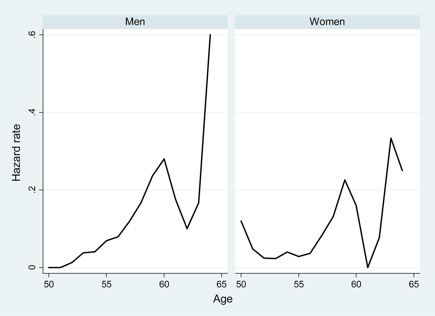
Our focus is on the retirement behavior of individuals working under the contractual wage earner scheme – by far the largest system in Belgium. Our sample consists of all individuals between the ages of 50 and 64 that are working as contractual wage-earners in either wave 1 or wave 2 of SHARE We pool observations and treat multiple years of observation for an individual as separate observations. We exclude self-employed and civil servants as well as retired, unemployed, sick and disabled people from the sample. We also exclude individuals who were not present anymore in SHARELIFE and for whom we do not have retrospective data. In total our sample consists of 1,403 observations, whose key characteristics are summarized in Table 1. The average age is 55 and a large majority of working men and women are living in couples. The average length of career is 33 years. Figure 5 summarizes the observed retirement hazards by age and sex for the sample, displaying rather large spikes at/around the key eligibility ages for men and women. For example, for women who are observed working at age 59 at the time of the survey, more than 20% withdraw from work within the following 12 months.

Figure 5. (Colour online) Retirement hazard rates, by age and sex. Source: Authors’ own calculations using SHARE.
Table 1. Descriptive statistics SHARE sample

Source: Authors’ own calculations using SHARE.
3. Methodology
The previous section illustrated that the retirement income of married individuals is strongly intertwined, rendering a purely individual approach problematic. However, the mechanical use of a Stock and Wise (Reference Stock and Wise1990) model would precisely do that by considering each person's own entitlements as separate from the spouses. The Belgian system is a good illustration of the issues that arise: when a spouse has an own pension that is lower than the spousal supplement of the partner, the spouse would show up with ZERO income in administrative data (and likely also in surveys), though economically speaking the person is collecting benefits – though on the name and the account of his or her partner.
We propose to revisit the incentive debate by using a couple-based incentive indicator rather than a purely individual one. The way (retirement) benefit systems takes into account the spouse's situation has an obvious impact on the household budget constraint and also on the individual's and the spouse's work and retirement decisions (see, e.g., Atalay and Barrett, Reference Atalay and Barrett2016). In many cases, the amount of current and future retirement benefits is directly related to the household composition and the employment and income status of the spouse. Blundell et al. (Reference Blundell, Chiappori and Meghir2005) and Cherchye et al. (Reference Cherchye, De Rock and Vermeulen2012) illustrated the importance of collective models of labor supply decision-making at a general level, while Michaud and Vermeulen (Reference Michaud and Vermeulen2011) worked on the special case of older workers’ labor supply. Blau (Reference Blau1998), Gustman and Steinmeier (Reference Gustman and Steinmeier2000) and Maestas (Reference Maestas2001) found evidence of joint retirement, defined as the coincidence in time of spouses’ retirement dates, which could be interpreted as complementarity in leisure among spouses.
In this paper we propose a consistent approach, whereby each partner considers optimizing his or her retirement date in order to maximize household-level resources taking the other partner's behavior as given. If the other spouse has not yet retired, we suppose that (s)he will do so at the earliest possible date, given available retirement options. We compute retirement incentives explicitly integrating the impact of a partner's retirement decision on the other partner's retirement income.Footnote 12 For ease of notation, we illustrate our approach below using the case of a married couple of retirees. Given the eligibility rules described in Section 2, the total couple pension income, P couple, at any given point in time– irrespectively on who is the payment beneficiary corresponds to
 $$\eqalign{P^{{\rm couple}} = & \,P^{{\rm single,\;} \;{\rm individual}} + P^{{\rm single,\;} \;{\rm spouse}} \cr & + {\rm max[}\max (P^{{\rm single,\;} \;{\rm individual}}, \;P^{{\rm single,\;} \;{\rm spouse}} )\cr & \times 0.25 - \min (P^{{\rm single,\;} \;{\rm individual}}, \;P^{{\rm single,}\;{\rm spouse}} ),\;0{\rm ]}} $$
rather than the mere P single,individual or P single,spouse. Beyond the case of pure singles, the latter amounts are also applicable to married couples with one partner retired and one working.
How does this change of pension concept affect key incentives? As a first indicator, we define couple pension or SSW as the present discounted value of all future entitlements that a person – or the couple – could have within the context of the various relevant (early-) retirement programs. For example, the SSW at time t for a single individual exiting the labor market through the pension system is given by
 $${\rm SSW}_t = \mathop \sum \limits_{i = t}^T \beta ^{i - t} \pi _i P_i^{{\rm single}} $$
where β is the intertemporal discount factor and π is the conditional survival probability to reach the age i. T is the maximal age at death and P single is the pension benefit, as in equation (1). We assume that the various benefits in payment remain constant in real terms, broadly in line with the price indexing of benefits in Belgium. The SSW takes into account the respective survival probabilitiesFootnote 13 of the relevant individuals and a financial discount rate across time (that we fix at 3% real, for illustrative purposes). In the case of a couple, the SSW integrates also spousal and survivor benefits:
 $${\rm SSW}_t = \mathop \sum \limits_{i = t}^T \beta ^{i - t} \pi _i P_i^{{\rm couple}} + \mathop \sum \limits_{i = t}^T \beta ^{i - t} (1 - \pi _i )\pi _i^{{\rm spouse}} S_i $$
where S stands for the survivor benefits and π spouse is the spouse conditional survivor probability. The same calculation is made for the other exit routes and, again, using a stylized notation, we can summarize the SSW of the couple as the weighted sum of the SSW of the different retirement income pathways (where q represents the respective probability weight of the respective pathway).
 $$\eqalign{{\rm SSW}^{{\rm couple}} = & \; q_{{\rm individual}}^{{\rm pension}} {\rm SSW}_{{\rm couple}}^{{\rm pension}} {\rm +} \,q_{{\rm individual}}^{{\rm unem}} {\rm SSW}_{{\rm individual}}^{{\rm unem}} \cr &{\rm +} \,q_{{\rm individual}}^{{\rm disab}} {\rm SSW}_{{\rm individual}}^{{\rm disab}} \hskip4pt {\rm +} \,q_{{\rm individual}}^{{\rm early}} {\rm SSW}_{{\rm individual}}^{{\rm early}} \cr &{\rm +}\, q_{{\rm spouse}}^{{\rm unem}} {\rm SSW}_{{\rm spouse}}^{{\rm unem}} {\rm +}\, q_{{\rm spouse}}^{{\rm disab}} {\rm SSW}_{{\rm spouse}}^{{\rm disab}} {\rm +}\, q_{{\rm spouse}}^{{\rm early}} {\rm SSW}_{{\rm spouse}}^{{\rm early}}} $$
SSWcouple thus improves on the individual SSW indicator as it integrates both partners’ survival-contingent income streams.
Figure 6 proposes an illustration of the impact of this change in indicators. It compares the individual and couple SSW computed for a sample of Belgian SHARE respondents, separated by sex. We allocate weights to the different pathways using administrative records on beneficiaries aged 50–64 in any given year as in Jousten et al. (Reference Jousten, Lefebvre, Perelman and Wise2016).Footnote 14 The graph illustrates that the couple notion leads to a substantial increase in evaluated financial resources as compared with a purely individualistic setting – and this particularly for women. Women's SSWindividual is low in line with lower observed labor force participation and lower hours of work over the lifecycle, as documented in Aliaj et al. (Reference Aliaj, Flawinne, Jousten, Perelman and Shi2016) and Fraikin and Jousten (Reference Fraikin and Jousten2016) with survey and administrative data, respectively. The improvement linked to the use of SSWcouple rather than SSWindividual is most pronounced for married women, who represent a large majority (93%) of the cohort under study. Expressed differently, it means that numerous married women are part of rather high income households, even if their own incomes taken individually would make them look like low income individuals. The results clearly show the importance of taking spousal and survivor benefits into consideration when evaluating people's future income levels.
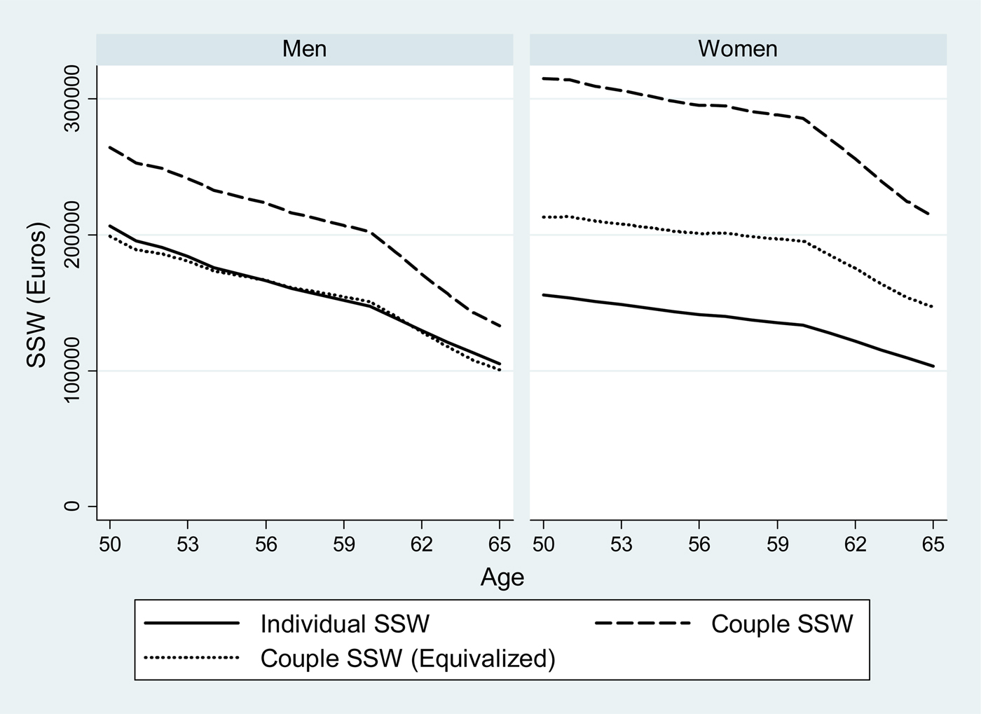
Figure 6. (Colour online) Average individual and couple SSW, by age and sex. Note: Prospective calculation for a sample of individuals aged 50 in wave 1. Source: Authors’ calculations using SHARE.
To complete the analysis, we propose couple income and SSW indicators that include equivalence scales. We use the modified OECD equivalence scale that assigns a value of 1 to the household head, of 0.5 to each additional adult member and of 0.3 to each child.Footnote 15 In our case, this implies that a couples’ total income is divided by a factor of 1.5 if both partners are alive, and by a factor of 1 in all other cases. The corresponding curves in Figure 6 document that scaling the SSW at the couple level has a substantial impact on the resources assigned to an individual. For women, the effect is most pronounced as a large share of household income is originating in the work and retirement income of their husbands: equivalized couple SSW is substantially lower than total couple SSW, but remains higher than individual SSW. For men, the situation is different, with equivalized couple SSW dropping to levels similar to the individual –level indicator – a sign that men's resources are contributing in a more pronounced way to both partner's well-being.
Beyond SSW, the change in our income retirement income variable also affects the specification of the Option Value (OV) model itself. In the classical OV model (Stock and Wise, Reference Stock and Wise1990) – and leaving aside survival probabilities for pure notational reasons – the value (utility) function of an individual when contemplating alternative retirement dates at any given time t is specified to be
 $$V_{t \vert h}^{{\rm single}} = \mathop \sum \limits_{a = t}^h ({\rm wage}_a^{{\rm individual}} )^\gamma + \mathop \sum \limits_{a = h + 1}^T k \times (P_a^{{\rm single,}\;{\rm individual}} )^\gamma $$
with h is the last year of work (and thus h + 1 the contemplated retirement age), k a leisure preference parameter, γ a risk aversion parameter and with an implicit assumption of no life-span uncertainty and no time-discounting for notational simplicity.Footnote 16 The OV is the difference between the function V single evaluated at the optimal retirement age minus its value upon immediate retirement.
Two major problems arise with this specification of the utility function when considering the case of couples. First, the specification includes a pension terms that could be composed of a single or a household pension – with no explicit or implicit recognition of differing household size. Second, the specification ignores the fact that, particularly for women, the true incentives might actually play not through one's own pension entitlement but rather through changes in the spousal benefit allocated to the partner.
We thus propose a change in the value function to reflect the household dimension. More specifically, household utility associated with any given retirement date h + 1 for a worker (evaluated at time t) corresponds to
 $$\eqalign{V_{t \vert h}^{{\rm couple}} = & \mathop \sum \limits_{a = t}^h ({\rm wage}_a^{{\rm individual}} + q_w^{{\rm spouse}} {\rm wage}_a^{{\rm spouse}} + (1 - q_w^{{\rm spouse}} ))^\gamma \cr &+ \mathop \sum \limits_{a = h + 1}^T k{^\ast}(q_w^{{\rm spouse}} (P_a^{{\rm single,\; individual}} + {\rm wage}_a^{{\rm spouse}} ) + (1 - q_w^{{\rm spouse}} )P_a^{{\rm spouse}} )^\gamma} $$
where  $q_w^{{\rm spouse}} $ is the probability that the spouse is still working during the period where the worker contemplates retiring. If the spouse is already retired,
  $q_w^{{\rm spouse}} = 0$, which is, for example, automatically the case as of age 65.
When projecting wages forward, we assume a constant real earnings profile – in line with the already mentioned assumption of real constancy on benefits in payment. We consider a Nash-like approach where the individual takes his or her partner's choice as given. The household OV indicator corresponds to the difference between the function V couple evaluated at the optimal retirement age of the worker minus its value upon immediate retirement.
Figure 7 documents the impact of this adaptation for household composition on the notion of OV for the same population of SHARE respondents as in the previous graph. It documents that the use of a couple notion lowers the value of the OV indicator – hence reducing the rewards to optimal retirement timing. This is particularly pronounced for women where the OV values turn more negative than men after age 60. These negative values for individuals aged 60+ means that for numerous married workers immediate retirement is the most rational choice as any individual gains in retirement incomes at the individual level are more than offset by losses on the side of the spouse. These findings further reinforce our previous observation of the relevance of integrating and interacting all benefits (including spousal and survivor benefits) for evaluating household resources.
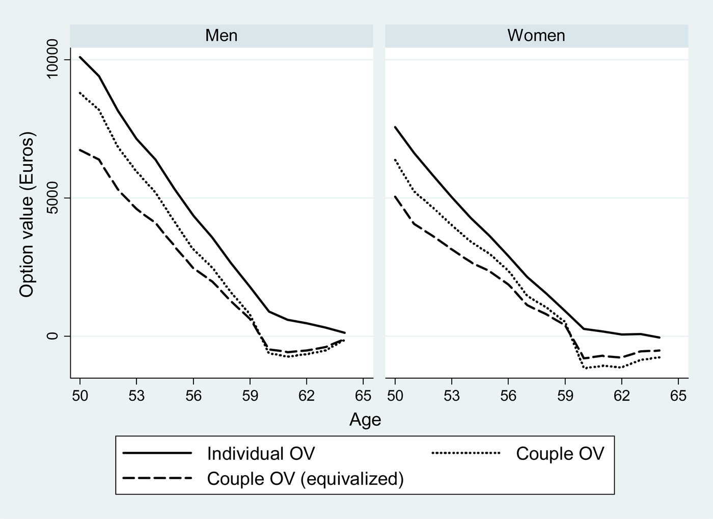
Figure 7. (Colour online) Average individual and couple OV, by age and sex. Note: Prospective calculation for a sample of individuals aged 50 in wave 1. Source: Authors’ calculations using SHARE.
Regarding the decrease in the dynamic incentive to retire, several elements are at play. First, by explicitly recognizing the interaction between spousal benefits, we better align the computed incentives to the true incentives faced by individuals. Second, couple and equivalized couple OV indicators better reflect the changing household size across different states of the world, in two conceptually different ways: while the former takes a grossing-up approach to including both partners income streams into the utility function, the second adds a scaling parameter to adjust the income (and hence utility) terms down to reflect the size of the household benefiting from a given income stream. Third, integrating the household dimension provides an implicit insurance to the individual, lowering the risks of suffering from low (or no) income outcomes. This third parameter hints at the influence of choosing specific utility function parameters – with more risk aversion leading to flatter profiles. Incentive profiles as a function of age are robust to changes in the parameter values of k and γ, and to differentiation between the sexes.Footnote 17
4. Estimation results
The results of probit estimations of labor market exits are presented and discussed below. The dependent variable takes the value of 1 if the individual is retiring within the year. We include the incentive variables of Section 3 as explanatory variables and we add a series of socio-demographic and economic control variables such as age, family status, education level, health, household wealth and income indicators of the individual/couple. Tables 2 and 3 summarize the results of different model estimates by means of the average marginal effect.
Table 2. Option value – probit – marginal effects

Note: Coefficients are the average of marginal effects. Standard errors in parentheses. *p < 0.1, **p < 0.05, ***p < 0.01. All regressions include control for net wage and lifetime earnings for the individual and for the spouse as well as squared of these variables and the interactions of these. Financial and real assets are also equivalized in the ‘equivalized’ regressions.
Table 3. Option value – probit by sex – marginal effects

Note: Coefficients are the average of marginal effects. Standard errors in parentheses. *p < 0.1, **p < 0.05, ***p < 0.01. All regressions include control for net wage and lifetime earnings for the individual and for the spouse as well as squared of these variables and the interactions of these. Financial and real assets are also equivalized in the ‘equivalized’ regressions.
Table 2 presents six specifications for a pooled dataset of men and women: two for individual, couple and equivalized couple indicators each. We differentiate according to the way age is introduced: linear or through dummies. The first columns present specifications in the spirit of Dellis et al. (Reference Dellis, Desmet, Jousten, Perelman, Gruber and Wise2004) and Gruber and Wise (Reference Gruber, Wise, Gruber and Wise2004) and reveal a strong and positive income effect, contrary to the findings of most contributors to this latter publication. As pointed by Belloni and Alessie (Reference Belloni and Alessie2009), it highlights the importance of having good quality data and careful imputation of transition. Previous studies for Belgium rely on administrative data that – though rich in some technical information - were likely not rich enough on other dimensions to correctly estimate the key parameters (e.g., wealth indicators).
The key results are not dependent on the age specification and are qualitatively similar. The coefficients of the age dummies are not reported here but are all non-significant except for the age 64 – which corresponds to an exit at the normal retirement age. For the rest, our estimates are consistent with previous findings with a negative effect of tertiary education and a strong positive effect of net financial wealth. Having an active spouse has a strong negative effect on retirement probabilities, lending support to the joint retirement hypothesis. Regional and health controls, as well as net real assets play no significant role.
Columns 3–6 replicate the same exercise for couples and equivalized couples, with broadly similar results for OV, SSW, and other key indicators. SSW seems to play a significant explanatory role in retirement decisions. Noticeable changes in the couples-specifications include a more powerful role of the ‘female’ dummy, which indicates that male and female incentives are likely different, and also differently affected by the use of broader couple-based incentive indicators. Column 6 further reveals that the equivalized couple specification has the advantage of better identifying the role of per capita household resources for the retirement decision – with the stronger marginal effect largely outweighing the underlying rescaling of income (and hence indirectly of SSW).Footnote 18
In Table 3 we separate the sample by sex and re-estimate the previous models using linear age specification by sex. In line with Dellis et al. (Reference Dellis, Desmet, Jousten, Perelman, Gruber and Wise2004), we find differences between the sexes. Contrary to these authors, we consistently find no significant role of social security incentive variables across all specifications for men- a finding that is very robust even to numerous robustness checks. For women, the OV and SSW indicators continue to play an important role, like in the pooled estimations reported in the previous table. Expressed differently, it looks like the pooled regressions’ findings of OV and SSW effects are mostly driven by women.
Men's retirement decisions are mostly a function of age, education and wealth levels, factors that play no or little role for women. Marital status and spousal activity indicators play no significant role for men, while they are strongly (negatively) significant for women. The strong negative effects of marital status is consistent with a view of the women as the secondary earner in the couple, having a much larger degree of freedom to choose the ideal retirement date for the couple. While male decisions seem to be mostly a function of exogenous factors, such as age, likely linked to the work environment in which they operate, their spouses have a much larger ability to fine-tune retirement in line with financial incentives, but also in line with their own perceived health situation and their spouses’ retirement decisions. Both types of couple estimations seem to capture these phenomena. In addition, equivalized couple indicators still keep their conceptual edge regarding the effect of household resources SSW over the simple couple indicator as for results in Table 2.
5. Conclusions
In the present paper, we studied retirement incentives on a sample of Belgian wage earners. We proceeded in three steps. First, we outlined some conceptual weaknesses of classical estimations using Stock and Wise (Reference Stock and Wise1990) option value methodology when applied to household types other than singles. We proposed methodological extensions to the baseline modeling of incentive indicators to better reflect the respective incentives faced by singles and couples. For couples, a key and often ignored dimension is the inclusion of the partner's benefits in assessing the level of well-being, as well as the crossed effects of one partner's behavior on the other's entitlements.
We derive two key sets of results. First, the introduction of modified incentive indicators for couples leads to substantial changes not only in terms of indicators of expected future income, but also in terms of dynamic retirement incentives. For numerous women, this broader view on entitlements leads to less work incentives – a contrast to previously estimated positive ones.
Second, we find empirical evidence of strong differences between the sexes. Using SHARE data from Belgium, probit models of retirement consistently reveal social security incentives playing a significant role for women, but not for men. For women – contrary to Gruber and Wise (Reference Gruber, Wise, Gruber and Wise2004) and others – our estimates further show an intuitively signed income effect of SSW that plays particularly strongly when using indicators relying on household equivalence scales.
Our results show that a more comprehensive approach to retirement incentives is warranted, particularly for couples. Our findings are consistent with a view that male labor market activity is largely of the primary-earner type, more strongly driven by exogenous factors with relatively little room for adjustment. Female labor market attachment is shown to be more heavily influenced by endogenous factors such as retirement incentives, self-perceived health and the partner's activity decision.
Appendix 1
Wage earners face three broad pathways to retirement: old-age pensions; unemployment and early retirement; sickness and disability. We cannot observe each individual's correct eligibility as it is a function of both worker and employer characteristics, such as information on periods of work, sector of work, etc.
As in Jousten et al. (Reference Jousten, Lefebvre, Perelman and Wise2016), we use weights based on observed exit patterns in the wage-earner population as a whole. More specifically, for each year of observation we use the share of the population for the age group 50–64 that is benefiting from unemployment, early retirement, disability benefits. Old age pension takes the residual such that the sum of the weights is equal to one. The choice of the 50–64 retirement-window is motivated by the fact that it corresponds to the main window of opportunity for retirement in Belgium.
The choice of a stock indicator of inactivity over an entire age range rather than a flow indicator by age is motivated by the fact that observed flows would either grossly over or under-estimate true eligibility for the individual retirement pathways depending on which assumption would be taken regarding those not retiring. An illustrative example might help illustrate the point. Consider the (extreme) example of a monotonous 1% of the total population retiring each year through the unemployment channel, and a further 1% through the disability channel over the age span 50–64. At age 50, taking our stock indicator, we would weigh retirement pathways as 15% on unemployment and disability each, and 70% on old-age retirement. Using a flow indicator, the respective weights would be 50/50/0% or 1/1/98% for unemployment/disability/old-age-pension respectively depending on whether we allocate the remaining 98% of non-movers to an early exit pathway or not.

Figure A1. Pathways to retirement – male wage-earners, age 50–64 (%). Source: INAMI, ONEM, ONP, Belgostat. Note: The denominator is the number of individuals in the same age group who were covered under the wage-earner regime and are currently inactive. The numerator is the split of these people across the various social security programs in the age group 50–64.

Figure A2. Pathways to retirement – female wage-earners, age 50–64 (%). Source: INAMI, ONEM, ONP, Belgostat. Note: The denominator is the number of individuals in the same age group who were covered under the wage-earner regime and are currently inactive. The numerator is the split of these people across the various social security programs in the age group 50–64.