3.1 Pension plan data

All state and local government employers, including the District of Columbia (DC), have Section 218 agreements with the Social Security Administration (SSA) that stipulate Social Security coverage. There can be significant confusion about which state and local government employees are covered by Social Security, even within SSA (GAO-10-938, 2010). Our teacher pension plan data come from the Center for Retirement Research, Public Pensions Database (PPD).Footnote ⁵

Table 1 lists the Social Security coverage status of teachers in each state and DC. There are 12 states plus DC where teachers are not covered by Social Security and 35 states where teachers are covered. The remaining three states, Georgia, Missouri, and Rhode Island, allow local school districts to enter into Section 218 agreements with SSA. Because teachers in those states cannot reliably be classified as covered or not, they are excluded from our sample.

Table 1. Teachers’ Social Security coverage by State

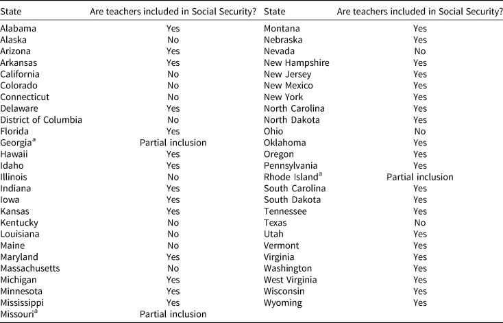
^a States where only some teachers are covered are excluded.

Notes: Pension plan data is derived from the Center for Retirement Research at Boston College's Public Plan Database. See Section 3.1 for details.

3.2 Teacher employment data

Data on the retirements are from the American Community Survey (ACS) from 2010 to 2016.Footnote ⁶ The ACS allows for the estimation of a large sample of teachers representative at the state level. Unlike administrative datasets, the ACS includes detailed demographics, marital status and household structure, and socioeconomic characteristics. Furthermore, the ACS allows for cross-state comparisons not possible with data from individual states. Because the employer can be imputed by the state of residence, we can merge on detailed information about pension coverage with reasonable accuracy. Longitudinal data, such as the HRS, provides a better indication of teaching history and teacher retirement. However, the ACS has a substantially larger sample size and allows for a more precise estimation of differences by public employer.

Following Harris and Adams (Reference Harris and Adams2007), teachers are defined as any individual who reported their most recent occupation as one of the following and who was also working in the last year: kindergarten teachers, primary and secondary school teachers, special education teachers, and other teachers not otherwise classified. This excludes all post-secondary teachers. We further restrict to those who report working for a state or local government employer.Footnote ⁷

The ACS contains limited information on work history necessitating an approximation of retirement. Failure to observe retirements will bias our estimates of the impact of Social Security inclusion if there is any correlation between the coverage of teachers by Social Security and moving into other work directly after leaving teaching. For example, the number of ‘unobserved’ retirements would be lower in non-covered states if individuals must work after retirement to supplement income. Similarly, Haider and Loughran (Reference Haider and Loughran2008) find that the Social Security Earnings Test reduces labor supply in retirement, although they do not consider specifically the timing of the return to paid employment. When a retirement is ‘missed’ by our measure, the denominator (i.e., the population of teachers) will also be lowered as that person is not identified as a teacher by our definition. As a robustness check, we confirm our main findings using a parallel analysis of teacher labor force participation rates. Labor force participation rates will not be biased by individuals transitioning directly from teaching to another position.

3.3 Means and descriptive statistics

Table 2 contains descriptive statistics for our sample of teachers by Social Security inclusion. Our sample is 88,788 teachers ages 50–70. Column (1) is the full sample. Column (2) includes teachers who are not covered by Social Security, as listed in Table 1. About 40% of teachers in our sample are not covered by Social Security. Column (3) includes teachers who are covered by Social Security. Column (4) provides the difference between Columns (3) and (2). To calculate the difference in means we conduct two-sided t-tests with the null hypothesis that Column (3) – Column (2) = 0. Standard errors are in brackets.

Table 2. Summary statistics

Notes: Teacher retirement data are derived from the 2010-2016 American Community Surveys, see text for details. The sample includes all teachers. Means are weighted at the person level with standard deviations in parentheses and standard errors in brackets.

*p < 0.10; **p < 0.05; ***p < 0.01.

The first row of Table 2 provides the average probability of retiring, i.e., teaching at some point in the prior year but no longer teaching at the time of the survey. On average, teachers ages 50–70 who are covered by Social Security are 0.65 percentage points (about 5% of the mean of the not-covered sample) more likely to retire than their peers who are not covered by Social Security. Given this, it is not surprising to see that, among 50–70 year olds who were working within the past year, the population of teachers covered by Social Security is slightly younger. Importantly, teachers in states covered by Social Security are 4.5 percentage points more likely to have an advanced degree. If Social Security inclusion is viewed as an amenity or state pensions are in better financial health in those states, teachers covered by Social Security may be positively selected. States where teachers are included in Social Security have more non-Hispanic African American teachers, while there are fewer Hispanic teachers. This is primarily driven by the fact that California and Texas are two large states not included in Social Security. The probability of being married is very slightly higher in states covered by Social Security, while the probability of being never married or divorced is lower. The regression estimates are insensitive to controlling for these demographic characteristics.

4.1 Age-specific retirement rates and survival probabilities

Figure 1 shows the retirement patterns of teachers separately by Social Security inclusion. This is contrasted with workers in ‘other occupations,’ most of whom will be covered by Social Security.Footnote ⁸ Note that some workers in this latter group will have had prior experience as a teacher, so we anticipate that the difference in retirement patterns in this other category of workers will be smaller but not necessarily zero.

Figure 1. Age-specific retirement rates for teachers and other workers.

Figure 1 illustrates that teachers are more likely than their private sector counterparts to retire between age 50 and 70 with the gap growing at about age 57 and increasing through the 60s. Second, there is a slightly higher rate of retirement after age 66 for other workers in states with Social Security coverage for teachers. This difference is much smaller than for those actively working as teachers and is likely due to prior public sector work among these ‘other’ workers. Most importantly, there is a striking difference in retirement rates between teachers covered by Social Security and those not covered. There is a jump at age 62, which coincides with the earliest age of eligibility to claim Social Security. The differences continue throughout the 60s with those covered by Social Security having a higher probability of retirement at each age except age 63.

To capture a clearer picture of the cumulative probability of retirement, Table 3 presents age-specific probabilities alongside a cumulative retirement rate.Footnote ⁹ Using a life table approach, we model the cumulative failure probability of a cohort of 1,000 workers actively employed at age 50. This approach is similar to Dudel and Myrskyl (Reference Dudel and Myrskyl2017) except it does not include adjustments for mortality. In Table 3, Column (1), we present age-specific retirement rates for teachers not included in Social Security, while retirement rates for those included in Social Security are in Column (4). To aid in interpreting these numbers, Columns (2) and (5) apply the age-specific probability of retirement to get a ‘failure’ rate that is the cumulative probability of retiring by the age in each row. We observe that the surviving number of teachers is always higher in states where they are excluded from Social Security. Furthermore, the cumulative retirement rate is always higher for teachers covered by Social Security. Importantly, the most dramatic differences occur at ages 62 and 66. We explore this further in a multivariate regression analysis below. Overall, this exercise provides suggestive evidence that Social Security coverage is associated with earlier retirements.

Table 3. Cumulative retirement probabilities by Social Security inclusion

Notes: Teacher retirement data are derived from the 2010 to 2016 American Community Surveys, see text for details. Age-specific retirement probabilities are presented in Columns (1) and (4). Using life table methodology, Columns (2) and (5) present the implied population remaining from a fictitious cohort of 1,000 teachers. Columns (3) and (6) translate these statistics into a cumulative retirement rate for the population.

4.2 Multivariate regression analysis

In the raw means presented in Table 3, we observe that retirement rates are generally higher for teachers who are covered by Social Security after age 62. We model this more formally by estimating versions of the following regression equation.

(1)$$\eqalign{\Pr ({\rm Retire}{\rm d}_{ist} = 1) =\,&F(\beta _{ss}SSInc_s + \gamma _a{\bf 1}(Age\,62-70)_{ist} \cr &+ \beta _a{\bf 1}({\rm Age}\,62-70)_{ist} \times SSIncl_s + X_{ist}\delta + P_{ist}\psi + M_{st}\theta + \tau _t)} $$

where i, s, and t index individuals, states, and years respectively. SSIncl _s equals 1 if an individual is in a state where teachers are covered by Social Security. ${\bf 1}(Age62-70)$ is an indicator of whether the individual is between ages 62 and 70. X _ist is a vector of individual characteristics. P _ist is a vector of state pension plan parameters that vary either across individuals or over time. M _st is a vector of state-level measures of macroeconomic conditions. Standard errors are clustered at the state level. The β _as are the parameters of interest.Footnote ¹⁰

We then present a more disaggregated model by age categories.

(2)$$\eqalign{\Pr ({\rm Retire}{\rm d}_{ist} = 1) =\,& F\bigg(\beta _{ss}SSInc_s + \sum\limits_{a = 60}^{70} {\gamma _a} {\bf 1}({\rm Ag}{\rm e}_{ist} = a) \cr &+ \sum\limits_{a = 60}^{70} {\beta _a} {\bf 1}({\rm Ag}{\rm e}_{ist} = a) \times SSIncl_s + X_{ist}\delta + P_{ist}\psi + M_{st}\theta + \tau _t\bigg)} $$

Age_ist is the age of individual i in state s in year t. This approach is similar to Asch et al. (Reference Asch, Haider and Zissimopoulos2005), where the authors estimate logit models of retirement regressed on peak and option value of retirement benefits along with a set of age-specific dummies.

We first estimate a baseline model with individual controls for sex, marital status, and education level. Social Security coverage is not the only aspect of retirement income that differs by state. To test the sensitivity of our findings, we add three pension characteristics and three proxies for state-level economic conditions to the baseline model. Means of these variables are provided in Appendix Table A1. We expect that states where teachers are not included in Social Security have different pension benefits. To capture some of the variations in plan characteristics, we define an indicator variable for theoretically being eligible for full retirement at the individual's age. For each pension plan in the data, we calculate the age at which a teacher who began working in the pension system at age 24 and had no breaks in service would be eligible for a full and unreduced pension. For this exercise, we utilize plan-specific retirement eligibility rules from the Urban Institute's State and Local Employee Pension Plan Database.Footnote ¹¹ We define the theoretical eligibility indicator as whether the individual is younger or older than that earliest full retirement eligibility age within their pension plan. Note that measure is just a theoretical construct as each individual's eligibility will be a function of age at hire and any prior service that might be used to purchase service. As shown in Appendix Table A1, among teachers who worked within the past year those covered by Social Security are more likely to be ‘eligible’ for a full retirement benefit, by this definition. This is consistent with teachers who are covered by Social Security being more influenced by Social Security eligibility than by pension plan parameters.

Additionally, we include two measures of pension plan health from the PPD: the funding ratio and the percent of employer's required contributions that was paid. The funding ratio measures the ratio of a pension plan's assets to its liabilities, so a higher funding ratio indicates a healthier pension. The percent of employer's required contributions that was paid measures the extent to which the pension plan sponsor pays its required contributions. A low value for this measure indicates that the cost of funding the pension plan may be causing fiscal stress for the sponsor. Along these two dimensions, plans included in Social Security are in better financial health.Footnote ¹²

To account for variation in macroeconomic conditions across states and over time we include controls for annual state unemployment rates, real GDP per capita, and per capita personal income. Again, means of these variables are provided in Appendix Table A1.Footnote ¹³ Note that while the unemployment rate is lower among states included in Social Security, real income per capita and real GDP per capita are both lower as well.

Table 4 presents estimated coefficients from a logit model estimating equation (1), with robust standard errors clustered by state of residence. The main estimated coefficients of interest are the age group indicator, the Social Security inclusion dummy variable, and the interaction between age and Social Security inclusion. All models also include year fixed effects, educational attainment (graduate degree), race/ethnicity, gender, and marital status. Marginal effects are reported in brackets at the bottom of the table. The marginal effects are calculated as the average change in probability from being included in Social Security for individuals ages 50–61 and for individuals ages 62–70. Column (1) includes only the baseline characteristics. Column (2) adds the three pension plan characteristics described above. The final column adds the three macroeconomic variables.

Table 4. Logit regression coefficient estimates

Notes: Teacher retirement data are derived from the 2010 to 2016 American Community Surveys, see text for details. The dependent variable is the probability of retiring in the past year. The specifications also include controls for gender and marital status, education, race/ethnicity. Standard errors clustered at the state level in parentheses.

*p < 0.10; **p < 0.05; ***p < 0.01.

First, the estimated coefficients on Social Security inclusion for the reference group (ages 50–61) are not statistically significantly different from zero. However, the confidence intervals on these estimates are large and include economically meaningful positive or negative differences. The bottom of the table presents the estimated marginal effects for ages 50–61 year olds. Again, these are economically small and not statistically significant. As expected, the estimated coefficient on the age group indicator suggests a large and statistically significant difference in retirement rates between the younger (ages 50–61) and older (ages 62–70) age groups. Importantly, the interaction term between the older age group and Social Security inclusion is positive and statistically significant. The marginal effects, reported at the bottom of Table 4, are calculated as the average change in probability of retirement from being included in Social Security for those ages 62–70. In the baseline Column (1), Social Security inclusion is associated with a 3 percentage point higher probability of retirement. The average probability of retiring among 62–70 year olds who are not covered by Social Security is 25%. Thus, the marginal effect suggests that, for teachers, Social Security eligibility is associated with a 12% higher probability of retirement, all else equal.

Because some teachers will be eligible for Social Security benefits through other jobs or through their spouse, this estimates represents a lower bound of the effect of Social Security eligibility on retirement. However, these estimates rely on cross-sectional variation across states. To determine the extent to which other omitted characteristics could explain these findings, we include three measures of pension characteristics in Column (2). As discussed in detail above, differences in employer-provided pension plan characteristics may be due to Social Security inclusion. Still, when controlling for these characteristics we observe a slightly larger effect of Social Security eligibility on retirement. Column (3) further includes macroeconomic conditions that vary by state and year. Again, including these controls suggests an even larger marginal effect. Note also that including the macroeconomic condition control variables changes the estimated time pattern of retirements. The constructed measure of ‘theoretical eligibility’ for full retirement benefits strongly predicts retirement, while the other two pension health measures do not. A higher unemployment rate is associated with an increased probability of retirement, but the other two proxies for macroeconomic conditions do not predict retirement, all else equal.

The results in Table 4 illustrate a statistically significant difference in retirement rates for individuals 62–70 by Social Security inclusion status. To further explore whether the age pattern of retirement rates differs by Social Security inclusion, we next disaggregate the age categories further as in equation (2). This more closely mirrors Figure 1. For this exercise, we construct the omitted age group as ages 50–59 and include age-specific dummy variables for ages 60–70. Column (1) of Table 5 presents these results. The specification here includes all covariates from Table 4, Column (3).

Table 5. Age-specific retirement patterns

Notes: Teacher retirement data are derived from the 2010 to 2016 American Community Surveys, see text for details. In Column (1), the dependent variable is the probability of retiring in the past year. Logit estimates are reported with marginal effects in brackets. In Column (2), the dependent variable is the teacher labor force participation rate, which is defined as the age × state × year × gender cell probability that an individual with at least a bachelor's degree is currently working as a teacher. Estimates are from an OLS regression. Both specifications also include controls for gender and marital status, education, race/ethnicity. Standard errors clustered at the state level in parentheses.

*p < 0.10; **p < 0.05; ***p < 0.01.

For the group of teachers not covered by Social Security, we observe that retirement rates increase monotonically in age except at age 69. Note that although most teachers with sufficient tenure will be covered by some form of retiree health insurance, Medicare is likely still an important component of health insurance support (see, e.g., Clark and Morrill, Reference Clark and Morrill2010).

The estimated coefficient on Social Security inclusion is again not statistically significant for the excluded age group (here ages 50–59), although the confidence intervals are large. The interaction terms between Social Security inclusion and age reveal a statistically significant difference in the retirement patterns of teachers. The estimated coefficients for the age-specific retirement rates are statistically significantly higher under Social Security eligibility at ages 62, 64, and 66. In Column (1), a Wald-test of the null hypothesis that the age 62–70 interaction coefficients are jointly equal to zero is rejected with p < 0.001. To give a sense of magnitude, in results not reported in the table, the average marginal effect of Social Security inclusion for a 62 year old (the sum of the baseline estimate plus the interacted term) is 4.8 percentage points. Table 3 showed the age-specific retirement rate for individuals age 62 who are not covered by Social Security is 19.14%. Thus, Social Security coverage is associated with about a 25% higher risk of retirement at age 62. To bolster our confidence in this conclusion, we perform a Wald-test of the joint null hypothesis that each of the age 63–70 interaction coefficients is equal to the age 62 interaction coefficient. We reject this null hypothesis at the <10% level with a p = 0.0693. These results indicate a clear impact of Social Security inclusion on the timing of retirement.Footnote ¹⁴

4.3 Labor force participation rates

So far, we have considered individual's transitions from working to not working. This ‘flow’ measure will capture all workers who retire from teaching and do not immediately begin a new job. The measure will not detect individuals who move directly from teaching to a new job without a period time spent not working. An alternative measure is a ‘stock’ of who is actively working as a teacher. For this exercise, we collapse the data into age × state × year × gender cells. We define the teacher labor force participation rate as the fraction of individuals in each cell who are actively working as a teacher.Footnote ¹⁵ We include in the numerator individuals who are currently employed or unemployed and report their current or most recent occupation to be a teacher. Individuals who report being out of the labor force are excluded from the numerator. The denominator is all individuals in that age × state × year × gender cell who have at least a bachelor's degree. All estimates are weighted by the population size of each cell. For age groups where the flow to stock ratio is small, it will be more difficult to detect a statistically significant change in the outflow from teaching. Still, we anticipate that the sign and approximate magnitude of the change will be similar to that from the preferred age-specific retirement rates analysis above.

To begin, we illustrate the teacher labor force participation rate for ages 25–70. Means are presented for each age individually with population weights used in the calculation of the mean.Footnote ¹⁶ Figure 2 illustrates that the teacher labor force is actually higher in states covered by Social Security for ages 25 through about age 55. For that age range, about 10% of individuals in states where teachers are covered by Social Security are working as teachers, compared with closer to 9% in non-covered states. This could be due to a labor supply effect indicating that Social Security is a benefit valued by potential teachers, or it could indicate something about the financial wellness of the state. This pattern switches starting at about age 55. Interestingly, from about age 55 through age 63, the teacher labor force participation rates are much more similar between the two groups of states. Starting at age 63, states where teachers are covered by Social Security have lower teacher labor force participation rates.

Figure 2. Teacher labor force participation rates.

Table 5, Column (2) presents estimates from an OLS regression with the same age-specific rate specification as in Column (1). Estimates weight each age × state × year × gender cell by the population size. The first row indicates that the teacher labor force participation rate does not significantly differ by Social Security inclusion for the omitted age group, ages 50–59. This is consistent with the labor force participation rate figure above. Similar to the retirement rate regressions presented above, the teacher labor force participation rates drop as individuals age. The estimated coefficients on age suggest a smooth decline in the probability of being a teacher by age with only a slightly larger decline at age 65.

To see the difference in participation in the teacher labor force by Social Security coverage, Table 5, Column (2) includes interaction terms with age and Social Security inclusion. Confirming the results above, Social Security is associated with lower teacher labor force participation rates starting at age 64. The estimate at age 62 is similar in magnitude but not statistically significant. Considering the most saturated model, shown in Table 5, Column (2), for individuals age 67, Social Security inclusion is associated with a 0.46 percentage point lower teacher labor force participation rate. The average labor force participation rate for non-covered teachers age 67 is 2.0%, shown in Appendix Table A3. This implies an approximately 23% lower teacher labor force participation rate among 67 year olds associated with Social Security coverage. Although not always statistically significant, the magnitudes are quite similar to that found analyzing retirement rates above. To put this number into perspective, Fetter and Lockwood (Reference Fetter and Lockwood2018) find that the OAA reduced the labor force participation rate of men in their late 60s by 8.5 percentage points.

The second half of Table 5 presents the estimated coefficients for the other covariates in the regression model. The time pattern for participation in the teacher labor force suggests a decline in teaching over time. Parallel to the results above, the unemployment rate is associated with a lower teacher labor force participation, potentially due to lower demand. Real GDP per capita (measured in thousands of dollars) is associated with a significantly lower teacher labor force participation rate.

4.4 Marital status

There are several reasons to expect retirement patterns for married individuals to be less sensitive to Social Security inclusion. First, own Social Security income may be a smaller portion of total household income and, thus, may be less important in timing retirement. Second, couples may consider other non-financial factors in timing their retirement, such as joint leisure. If so, we expect to see a smaller impact of financial incentives on retirement. Retirement coordination is well established in the data: married couples tend to retire at the same time (Blau, Reference Blau1998; Gustman and Steinmeier, Reference Gustman and Steinmeier2000; Coile, Reference Coile2004). This result is often explained by the joint budget set faced by couples and leisure complementarities between spouses. This intuition runs counter to recent empirical evidence which suggests that the returns to additional years of work later in life are greater for married women than for married men (Maestas, Reference Maestas2017). Henriques (Reference Henriques2018) uses Social Security records to estimate whether men and women claim Social Security benefits in a way that maximizes benefit levels. Her analysis shows that, despite the increase in women's labor force participation and wages, wives are still dependent on their husbands’ Social Security benefits. Further, she finds that husbands respond to their own incentives but do not claim in a way that maximizes dependent benefits.

One benefit of the ACS is that we can observe marital status and, if married, characteristics of the spouse. In Appendix Table A4, we present estimates for the samples of married women and married men, with controls for spouse's age and labor supply, parallel to our preferred model from Table 4, Column (3). Our empirical results lack sufficient power to estimate meaningful differences by gender and marital status. However, the estimates are suggestive that the impact of Social Security eligibility is larger for single women at younger ages and larger for married women and men later in their 60's.

In Appendix Table A4, Column (1), the marginal effect of Social Security coverage at age 67 indicates an 11.17 percentage point higher probability of retirement. Not shown in the table, the average retirement rate for married female teachers not covered by Social Security who are age 67 is 31.7%. Thus, Social Security coverage is associated with about a 35% higher probability of retirement among 67 year old married female teachers, but not at other ages. Married male teachers age 66 also have a statistically significantly higher probability of retiring if covered by Social Security. Here, the marginal effect of 10.50% represents about 47% of the non-covered mean of 22.3%. For married male teachers there are also statistically significant differences by Social Security coverage at ages 69 and 70. The fact that we do not see similar jumps at the early Social Security claiming ages for married men or women suggests that factors impacting the joint retirement decisions of couples might outweigh the effects of Social Security incentives. There is also evidence of a desire for joint leisure as having a spouse who is not in the labor force is associated with a large and statistically significantly higher probability of retirement for both men and women. Still, the standard errors on these estimates are large, so we do not explore this further in this context.