1.1 Self-reported data

All participants who report employment are asked about retirement plan coverage and plan characteristics (such as employer and employee contributions to DC plans or expected benefits from DB plans) at their current jobs. All new entrants are also asked about their employment history and any retirement plan coverage in their previous jobs.

As we show in the next section, the self-reported data contain significant errors. While we base our estimations of retirement wealth on the self-reported data on retirement plan type and plan characteristics at the current job, we use administrative data from W-2s and SPDs to identify and correct possible discrepancies.

1.2 Forms W-2

For participants who consented, the HRS data contains information from W-2s for years starting in 1978 up to the year of consent (or onwards in some cases) that can be used to project DC plan balances, given assumed investment returns and employer contributions. W-2 information for 1978 and 1979 is incomplete and is not used in our analysis. The share of workers matched to W-2s varies from 84% in 1992 to 39% in 2010. HRS survey participants are asked repeatedly to give permission to the HRS to link their W-2s with survey information. By 2010 almost all 1992 participants have given consent. The share of those consenting to a W-2 link is lower for more recent cohorts partly because they have been asked fewer times. The HRS has created reweights for the survey sample on the basis of observable characteristics associated with the probability of providing a consent to ensure that the sample is representative after the application of sample weights. We use such HRS created sample weights but acknowledge that our results may be affected by unobserved differences between consenters and non-consenters.

The W-2 forms are submitted annually by employers to the IRS and contain information, among others, on gross pay and the employee's elective deferrals to DC plans. W-2s do not contain information on the employer's contributions to DC plans, plan balances, loans or withdrawals, or information about IRA contributions or balances. While the self-employed do not have to file W-2 forms, the dataset also contains data on self-employment income that are derived from other tax forms, but it does not contain information on their retirement contributions.

Comparing self-reported DC plan participation with W-2 and SPD data indicates significant discrepancies, which we attribute to errors in the self-reports. The errors seem to lead to lower-than-expected retirement plan balances. Forms W-2 contains a series of box entries that researchers can use to identify or infer retirement plan contributions. In 1991, only 69% of workers whose W-2 contained elective deferrals (in Box 12) reported a DC plan. Participants who misreport plan type are asked questions relevant to their self-reported plan type but the responses aren't valuable. Average self-reported 401(k) balances in the HRS are lower than those reported in Investment Company Institute, Employee Benefit Research Institute, and other household surveys (Venti, Reference Venti2011). The HRS survey design likely contributes to under-reporting (Venti, Reference Venti2011). Errors in self-reported data, even if random, introduce noise, inflate estimates of retirement wealth inequality, and may also overstate increases in retirement wealth inequality resulting from the displacement of DB by DC plans if the average size of the errors in self-reported estimates of DC plan balances exceeds the average size of errors in projected DB income. In contrast, our assumption that all DC participants receive the same investment return conditional on asset allocation will understate the increase in inequality.

Though well-informed participants might provide more accurate estimates of their own plan balances than researchers, we consider the estimates based on W-2s and assumed investment returns to be superior to self-reported balances. But the use of W-2 data has some limitations. Though information on elective deferrals is contained in Box 12 on the W-2, these data are not available for all participants or years. For years and participants lacking Box 12 data, previous studies have inferred elective deferrals by comparing Box 1, earnings subject to federal income tax, which exclude elective deferrals, with Box 5, Medicare taxable earnings, which includes deferrals. However, Medicare taxable earnings were capped prior to 1994 so that the difference between Box 5 and Box 1 would understate the employer-sponsored retirement plan contributions of high earners in those years. In addition, employer-sponsored retirement plan contributions were deductible for both income tax and Medicare tax purposes prior to 1984 so that for these years Box 1 equals Box 5. Further, employee contributions to state and local DB plans are also deductible when calculating Box 1 so that a comparison of Box 5 with Box 1 will overstate state and local government workers' DC contributions. In addition, box entries are sometimes missing or inconsistent – for example on occasion Box 1 exceeds Box 5 – and we drop these observations.

Methods used by previous researchers to estimate employer-sponsored retirement plan contributions are unsatisfactory for the purposes of measuring inequality. Dushi and Honig (Reference Dushi and Honig2010) drop workers with earnings above the Medicare earnings cap. Dropping high earners makes sense when analyzing the broad mass of the population, but less so when investigating inequality. Cunningham and Engelhardt (Reference Cunningham and Engelhardt2002) and Dushi and Honig (Reference Dushi and Honig2015) aim to eliminate state and local government workers from the sample but that biases estimates of retirement wealth inequality, because state and local government workers have relatively generous pensions. Dushi and Honig (Reference Dushi and Honig2010) include state and local workers without attempting to adjust Box 5–Box 1 calculation. We include all workers and adjust Box 5–Box 1 calculation of those we identify as state and local government workers which improves on previous attempts to identify likely state and local government workers. We identify them by comparing Box 5–Box 1 calculation with Box 12 for years for which Box 12 data are available.

1.3 SPDs

In order to overcome problems with self-reports, the HRS staff sought to collect SPDs from individuals who report, sometimes in error, that they are participating in an employer-sponsored retirement plan. The SPDs summarize rules of DB, DC, stock option, and profit-sharing plans. DB plans require participation, but 401(k)-type plans are voluntary so that a correctly matched DC SPD shows a worker is eligible but not whether they participate. Although the probability of an SPD match varies with worker characteristics, the HRS has not constructed weights, similar to the W-2 weights, to deal with selection. We deal with the selectivity issue with regard to SPDs by imputing employer-sponsored retirement plan coverage and wealth using available information from self-reported data and W-2s, but acknowledge that workers matched to SPDs may differ in ways that can't be observed from those who are not matched.

Self-reports and the SPDs often conflict (see Table 2).Footnote ¹ To illustrate the conflict, row three of Table 2 reports that in 1992, of workers who stated they had both DB and DC plans, 27.4% were unmatched, 35.3% were matched only to a DB SPD, 9.5% only to a DC SPD, and 27.8% to both DB and DC SPDs.

Table 2. SPD type by self-reported plan type and wave

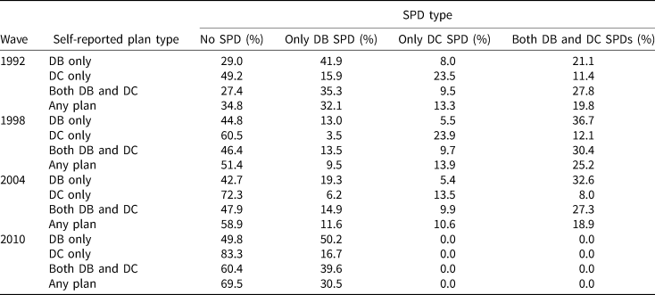
Note: Self-reported plan types are extracted from RAND HRS. No sample weights, to provide comparability with Gustman et al. (Reference Gustman, Steinmeier and Tabatabai2010). Sample includes all workers who joined in the relevant wave and self-report having a retirement plan in their current job.

The HRS did not collect DC SPDs in 2010; hence, there is no DC match rate in that wave. The HRS data do not distinguish between workers for whom the HRS failed to obtain any SPDs, and workers whose employers stated they did not sponsor a retirement plan. The match rate in earlier years is non-random (Gustman and Steinmeier, Reference Gustman, Steinmeier, Gale, Shoven and Warshawsky2004). The 20.1% of workers reporting only a DB plan who were matched to both DB and DC SPDs may be correct because they may be eligible non-participants. Gustman et al. (Reference Gustman, Steinmeier and Tabatabai2007, Reference Gustman, Steinmeier and Tabatabai2010) attribute mismatches that cannot be explained by eligible workers not participating in worker mis-reporting. But we question their conclusion. Among individuals reporting only being covered by a DB plan, 21.8% have W-2 deferrals, revealing a DC contribution (Table 3). Among individuals matched only to a DB SPD, a larger share, 40.7% have W-2 deferrals, reflecting missing DC SPDs, so that the self-report of DB coverage is a superior measure.

Table 3. Percentage with non-zero W-2 elective deferrals in 1991 by self-reported plan type and SPD type in 1992 wave

Note: Sample includes all respondents with available W-2 information in 1991.

If we relied solely on the self-reports of workers with a matched SPD, we would incorrectly classify 24% of workers who have W-2 deferrals as not having a DC plan. In contrast, if we relied solely on SPDs, we would incorrectly classify 45% of workers with W-2 deferrals as not having a DC plan. We conclude that SPDs cannot be relied on to the exclusion of self-reports and W-2s.

1.4 Pension estimation program

The SPDs specify plan rules, benefit formulas, and plan changes. Since they do not contain data on individuals, the HRS created a PEP for users to estimate DB and DC wealth by combining SPD data with self-reported data on earnings and deferrals (Rohwedder, Reference Rohwedder2003). The HRS PEP has five significant drawbacks. First, when calculating DC wealth, the user must choose a constant real rate of return, common to all participants – the default rate is 2.9% in 2010 – which ignores individual differences in asset allocations and investment returns. Second, the PEP extrapolates a wage history from current year earnings after the user defines the constant rate of real wage growth common to all participants – the default is 1.1% a year in 2010. This process will misreport earnings to the extent that current year earnings are mis-reported or earnings growth differs from the assumed rate. Third, the PEP assumes a time-invariant voluntary contribution rate to 401(k)-type plans equal to the most recent self-reported contribution rate, which overstates the DC wealth of current contributors if participation rates have grown over time or workers have taken participation holidays. Even small errors in assumptions can have a dramatic effect on DC wealth estimates (Rohwedder, Reference Rohwedder2003). Fourth, the PEP disregards in-service withdrawals and 401(k) loan defaults that amount to perhaps 0.5% of 401(k) wealth a year, which is significant over a career (Munnell and Webb, Reference Munnell and Webb2015). Fifth, the PEP does not deduct outstanding loans. Although about 90% of active participants can take out DC loans (VanDerhei et al., Reference VanDerhei, Holden, Copeland and Alonso2012) and about 18% of participants in plans offering loans had a loan outstanding (Vanguard, 2014), loans amounted to only 2% of plan assets. We proffer the likelihood that loans increase retirement wealth inequality but do not investigate because the HRS survey instrument does not ask about retirement plan loans.

To correct the first three problems and coding anomalies, Cunningham, Engelhardt, and Kumar (Reference Cunningham, Engelhardt, Kumar, Madrian, Mitchell and Soldo2007) (CEK) created their own PEP to estimate DC wealth for 1992 and 1998. Their PEP uses W-2 data on earnings and elective deferrals; uses the plan adoption and amendment dates indicated in the SPD to determine a person's eligibility for certain plan features; and incorporates a user-defined time-varying rate of return. Convinced by CEK's findings that the HRS PEP systematically overstates DC wealth, we use their methods.

The HRS PEP calculates the expected present value of DB wealth – DB benefits are typically a function of current or recent salary, age, and years of service – by combining self-reported data with plan rules obtained from the SPDs and assumed mortality and interest rates. Wealth is discounted back to the present and we prorate between past and anticipated future service. The HRS PEP allows users to calculate DB wealth with normal or early retirement formulas within a user-defined age range. These calculations introduce the following measurement errors. First, reporting errors in self-reported earnings will be reflected in DB wealth estimates. Second, older workers often experience earnings declines (Rohwedder, Reference Rohwedder2003), whereas the HRS PEP assumes a constant rate of real wage growth right up to retirement. As benefits are typically based on final salary or the average of the last few years' salary, the HRS PEP probably overstates DB wealth, except for those near retirement.Footnote ² Third, the HRS PEP does not incorporate the risk of premature job-separation, which can substantially reduce DB wealth. Almost half of workers retire before they expect (Munnell et al., Reference Munnell, Sanzenbacher and Rutledge2015).

We replace self-reported earnings data with W-2 data. While modeling wage trajectories and the risk of premature job-separation of DB participants is beyond the scope of this study, we instead make ad-hoc adjustments for risk by discounting future benefits at the corporate bond interest rate rather than at the risk-free Treasury bond interest rate.

For 2010, the HRS PEP allows researchers to impute DB wealth to workers without DB SPDs. Using this option, Fang et al. (Reference Fang, Brown and Weir2016) assign DB coverage to all workers either matched to a DB SPD or who self-report DB coverage. Their approach will overstate total DB coverage when workers covered only by DC plans misreport being covered by a DB plan.

2.1 Studies of coverage

Self-reported data from the Current Population Survey (CPS) reveal that only about 50% of full time private sector workers participate in an employer-sponsored retirement plan at any point in time, with the participation rate trending down (Munnell and Bleckman, Reference Munnell and Bleckman2014).Footnote ³ Workers move in and out of coverage, so the share ever covered is higher. Lower-income workers are less likely to participate, with the socioeconomic pension coverage gap mainly reflecting lower eligibility rates among low earners (Karamcheva and Sanzenbacher, Reference Karamcheva and Sanzenbacher2010; Wu and Rutledge, Reference Wu and Rutledge2014).

An alternative approach to relying solely on self-reported data, designed to address mis- and under-reporting, is to combine self-reported data with data from W-2s (Dushi et al., Reference Dushi, Iams and Lichtenstein2011). But workers who report participating in a DC plan but do not have W-2 deferrals could have a DC plan that does not require employee contributions, could have mistakenly reported their DB plan as DC, or could have no retirement plan coverage. Assuming they have no employer-sponsored retirement plan coverage yields coverage rates in line with self-reported data, whereas assuming they are participating in some other plan type yields higher coverage rates. We conclude the CPS data represent a lower bound to a range of coverage estimates.

Another approach is to rely solely on IRS Statistics of Income data, classifying workers as covered if employer-sponsored retirement plan elective deferrals are shown in Box 12 of the W-2 or if Box 13 has been ticked, indicating active participation in any type of employer-sponsored retirement plan (Brady, Reference Brady2017). These data show a participation rate that is consistently 4–6 percentage points higher than the comparable CPS participation rate.Footnote ⁴ Box 13 is not included in the HRS W-2 dataset and we therefore cannot use their approach.

2.2 Studies of contribution rates and asset allocations

Conditional on participation, the average DC employee contribution rate is 6.5% of salary (Brady, Reference Brady2017). Contribution rates are higher for older workers but vary little with earnings. High earners and younger workers are more likely to hold equities but differences in mean equity shares are modest. The mean share in company stock declined from 11% in 2007 to 6% in 2016 and there is substantial individual-level heterogeneity in investment allocations, with significant shares of participants with equity allocations of zero or 100% (VanDerhei et al., Reference VanDerhei, Holden, Alonso and Bass2018). As equity returns have exceeded those on bonds, differences in asset allocation likely contribute to inequality.

Conditional on the employee participating, higher earners receive larger employer matches as a percent of salary (Saad-Lessler et al., Reference Saad-Lessler, Ghilarducci and Resnik2018). Given that employee contribution rates vary little with earnings; this likely reflects differences in the generosity of match formulas.

2.3 Studies of retirement wealth

Studies of retirement wealth (IRA, DB, and DC wealth, excluding the expected present value of anticipated Social Security benefits) typically use Survey of Consumer Finances (SCF), Survey of Income and Program Participation (SIPP), and HRS data. Studies typically include IRA account balances because although IRAs are not employer sponsored, most IRA wealth represents rollovers from DC plans, not direct contributions. We do not regard the HRS age restriction as a significant drawback because we measure the distribution of retirement wealth of households approaching retirement. The CPS asks about employer-sponsored retirement plan coverage but not wealth. The SCF contains a high-wealth sub-sample to investigate the upper tail of the wealth distribution, but the lack of either a panel or a link to administrative data makes it unsuitable for describing the relationship between retirement wealth and lifetime earnings.Footnote ⁵ And the SCF likely suffers from the same level of misreporting of pension type as the HRS does.

Two consistent findings emerge. First, employer-sponsored retirement wealth is highly unequally distributed, although less unequally distributed than non-retirement financial wealth (Wolff, Reference Wolff2015; Devlin-Foltz et al., Reference Devlin-Foltz, Henriques and Sabelhaus2015a, Reference Devlin-Foltz, Henriques and Sabelhaus2015b). Using 2014 SIPP data and a broader sample, Ghilarducci et al. (Reference Ghilarducci, Papadopoulos and Webb2017) report that one third of workers nearing retirement have no employer-sponsored retirement wealth. Government Accountability Office (GAO, 2014) reports that 1% of IRA holders with balances in excess of $1 million hold 22% of IRA wealth. Employer-sponsored retirement wealth is also more unequally distributed than current period earnings (Mitchell and Moore, Reference Mitchell and Moore1997) and total wealth varies enormously even within lifetime earnings deciles (Venti and Wise, Reference Venti and Wise1998).

Second, although DC wealth was substantially more unequally distributed than DB wealth in all years, the displacement of DB by DC plans has not been associated with a significant increase in retirement wealth inequality (Wolff, Reference Wolff2015; Devlin-Foltz et al., Reference Devlin-Foltz, Henriques and Sabelhaus2015a, Reference Devlin-Foltz, Henriques and Sabelhaus2015b; Munnell et al., Reference Munnell, Hou, Webb and Li2016b).

Although higher-income earners have lower replacement rate targets, their lower Social Security replacement rates mean they need to accumulate larger multiples of their earnings. Including Social Security wealth, the ratios of mean and median employer-sponsored retirement wealth to earnings vary little by lifetime earnings decile. The ratio of DC wealth to lifetime earnings is higher in the upper lifetime earnings deciles; whereas the ratio of DB wealth to lifetime earnings is lower (Poterba et al., Reference Poterba, Venti and Wise2007, using 2000 HRS data). But this pattern masks enormous differences in wealth, conditional on lifetime earnings (Venti and Wise, Reference Venti and Wise1998, using 1992 HRS data and focusing on total wealth excluding Social security and financial wealth excluding retirement accounts). Most inequality in employer-sponsored retirement wealth stems from differences in outcomes within lifetime earnings groups.

The study most similar to ours is Munnell et al. (Reference Munnell, Hou, Webb and Li2016b), which analyzed household HRS data from 1992, 1998, 2004, and 2010 and sorted households by quartile of educational attainment (not lifetime earnings), relied solely on the self-reported data, and did not examine the distribution of employer-sponsored retirement wealth within quartiles. Consistent with previous research, the Munnell, Hou, Webb, and Li study found that DC wealth was more skewed towards the top quartile of educational attainment than DB wealth, but that the distribution of total employer-sponsored retirement wealth by education quartile barely changed over the 18-year period, notwithstanding the displacement of DB by DC wealth.

2.4 Comparing wealth accumulation under DB and DC plans

DC wealth of pre-retirees falls far short of DB wealth (Munnell et al., Reference Munnell, Hou, Webb and Li2016b; Ghilarducci et al., Reference Ghilarducci, Papadopoulos and Webb2017). Some of the disparity likely reflects the immaturity of the DC system – older workers have not had a lifetime of exposure. But leakages, high fees, and portfolios not located on the efficient market frontier also contribute to the failure of DC plans to live up to their promise (Tang et al., Reference Tang, Mitchell, Mottola and Utkus2010; Munnell and Webb, Reference Munnell and Webb2015), as does non-participation by eligible workers.

In contrast, a well-functioning DC system might engender greater wealth accumulation than a DB system, because job-changers are not penalized. Using HRS data on earnings histories and job-separations, Poterba et al. (Reference Poterba, Rauh, Venti and Wise2006) compare retirement wealth in DB and DC plans. They randomly assign participants first a DB plan and then a DC plan. They assume that vested DB participants receive a deferred pension on job-separation based on their salary at the date of separation. The DC simulations assume zero leakages, and no periods of non-participation. They find that even in risk-adjusted terms, DC plans almost always dominate private sector DB plans.

The Poterba et al. (Reference Poterba, Rauh, Venti and Wise2006) assumption of zero leakages and 100% participation will likely understate DC wealth inequality as will the assumption that all participants earn the same investment returns. Even with these restrictive assumptions, they find that DC plans produce greater inequality (as measured by the ratio of the 90th to the 50th percentile of the wealth distribution) than DB plans.

More generally, those approaching retirement in 1992 were not living in a ‘golden age’ of pensions, due to patchy DB coverage and erosion of benefits by inflation and pre-retirement job-loss (Kolodrubetz and Landay, Reference Kolodrubetz and Landry1973). In addition, low earners get lower benefits from ‘integrated’ DB plans – employers count Social Security benefits as part of the total benefit, which can also foster between-group inequality.

3.1 DB wealth from current job

We use the HRS PEP to calculate the expected present value of current job DB wealth for plans for which DB SPDs are available. We consider the W-2 earnings data more reliable than self-reported data and therefore modify the HRS PEP to calculate DB wealth using W-2 earnings data. We discount at the AAA corporate bond interest rate (7.92% in 1992, 6.40% in 1998, 5.46% in 2004, and 4.53% in 2010) and pro-rate to past service. Friedberg and Webb (Reference Friedberg and Webb2005) show employees' retirement timing decisions are influenced by DB wealth accrual. We assume employees retire when first eligible for normal retirement benefits, an age at which the expected present value of benefits often peaks. We did not use a constant interest rate across years because we want to preserve within-wave comparability with DC wealth, the value of which reflects prevailing interest rates. We use the HRS PEP default real wage growth assumptions of 0.96 to 1.1% a year to retirement.

We assume no DB SPDs were erroneously matched and that if the HRS matched a DC plan, which indicates the HRS successfully identified and contacted the employer, but did not match a DB plan, the worker is not covered by a DB plan, regardless of self-reported plan type. We impute DB coverage for those without any SPDs using a donor pool of those matched to any SPDs and a comprehensive set of covariates that include self-reported plan type and characteristics associated with a SPD match. Importantly, to create an appropriate joint distribution of DB and DC coverage, the set of covariates includes a variable indicating whether the worker made W-2 elective deferrals.

Our approach will likely create an upward bias to DB coverage because those with DB SPDs are more likely to have DB plans than those without (conditioning on covariates).Footnote ⁶ We adjust the coverage rate by recoding as DC those who report being covered only by a DC plan and have W-2 elective deferrals. After this adjustment, we obtain an overall DB coverage rate that matches that observed in the self-reported data, although the identities of covered workers differ.

3.2 DB wealth from past jobs

While some SPDs from previous jobs are available for the 1992 and 1998 waves, the HRS did not collect SPDs for past jobs in 2004 and 2010. The match rate is low – in 1992, only 26% of workers reporting that they anticipated future benefits from a DB plan from a past job were matched to an SPD. We therefore use Gustman et al. (Reference Gustman, Steinmeier and Tabatabai2014) estimates of DB wealth from past jobs, including DB pensions in payment, based on self-reported data. In 1992, only 9.4% of workers had DB wealth from past jobs (including DB pensions in payment) so that any errors in self-reported data will have only a modest effect on total retirement wealth.

3.3 DC wealth from current jobs

To calculate current job DC wealth resulting from employee contributions, we combine W-2 data on gross pay and elective deferrals with self-reported data on hire date and DC plan asset allocation and Ibbotson (2018) data on market returns by asset class.

We rely on W-2 Box 12 data, where available. For workers for whom Box 12 data are available for 1991 onwards, we estimate pre-1991 deferrals by comparing the 1991 Box 12 entry with the 1991 difference between Box 5 and Box 1. If Box 12 equals zero, we assume the difference between Box 5 and Box 1 in all previous years represents employee DB contributions. If Box 12 equals Box 5 minus Box 1, we assume the difference between Box 5 and Box 1 represents DC elective deferrals. In all other cases, we make an apportionment. We experimented with using SPDs to identify employee contributions to DB plans but found that this approach could only explain a small part of the difference between Box 12 and Box 5 minus Box 1.Footnote ⁷

Box 5 minus Box 1 calculation cannot be applied prior to 1984 because Social Security and Medicare taxes were calculated on earnings net of elective deferrals. We assume zero employee contributions in 1981 and linearly interpolate coverage rates between 1981 and 1984, the first year for which data are available. For workers with earnings above the taxable maximum in any of the years 1984 to 1990 or 1991, we impute iteratively, working back from the most recent year, using data from time t + 1 to impute time t to capture serial correlation in deferrals.

For workers for whom Box 12 data were not collected in 1991 or afterwards, we impute employee contributions using Box 5 and Box 1 data from a donor pool of workers whose DC contributions were based on the methodology described above. The W-2s contain the most accurate information on employee contributions; therefore we disregard the self-reported data when it contradicts.

For employer contributions, we considered and rejected using matched or imputed SPDs. The DC SPD match rate is low in earlier years and likely biased in favor of larger plans, and DC SPDs were not collected in 2010, which means DC wealth for that wave must be constructed solely from self-reports. Also, DC plan type – profit sharing, money purchase, 401(k), etc. – needed to impute SPDs, is often missing or likely misreported.

We use a worker being matched to a DC SPD as one indicator of a worker having a DC plan, regardless of what a worker self-reported as their plan type. But we don't use SPD information to calculate DC wealth from employer contributions. Instead, we use self-reported data to calculate employer DC contributions.

To provide consistency with actual and imputed data, we impute employer contributions to DC plans for workers who did not report employer contributions, but may have them. These workers include those who (1) say they have a DB plan but are not assigned a DB plan, or are matched to a DC SPD, (2) don't have W-2 contributions, are not assigned a DB plan, and report no employer contribution, and (3) those who say they have a DC plan but don't answer the subsequent questions.

3.4 DC wealth from past jobs and IRA wealth

When workers leave their jobs they can withdraw their 401(k) plan balance, roll the money into an IRA, leave the money invested in the old plan, or, more rarely, move their 401(k) into a new employer's 401(k). (Very few choose multiple options [Vanguard 2014]). HRS participants are asked how much was in their account when they left their employer, which of the above options they chose, and if they rolled over the balance into an IRA or left it in the original plan, how much is in the account now.

The HRS collected DC SPDs for some previous jobs. We choose not to use W-2s and SPDs to calculate current wealth from past jobs for two reasons. First, significant leakages and transfers likely occur not only at job separation but also after they get a new job. Second, most DC wealth is now held in IRAs, not in 401(k)s (Munnell and Webb, Reference Munnell and Webb2015), especially among older workers who have changed jobs several times during their career. These IRAs commingle rollovers from possibly several past jobs with direct contributions. Using W-2 and SPD data to estimate current wealth from past jobs would create a new issue – how to calculate the share of the IRA balance that related to that past job. We consider that, even with reporting error, the self-reported current account balance will generally be a more accurate measure of current DC wealth from past jobs than calculations based on SPDs and W-2s. We therefore use imputed values of IRA wealth from the RAND HRS Longitudinal File. We use Gustman et al. (Reference Gustman, Steinmeier and Tabatabai2014) data constructed using self-reported data on DC wealth from previous jobs, not rolled over to IRAs.

3.5 DC investment returns

In 1992, 1998, and 2004, participants in 401(k) type plans report whether the money in each of their accounts is invested mostly in stocks, mostly in interest earning assets, or is about evenly split. In 2010, they are asked to report the percentages invested in stocks. We impute missing asset allocations for 2010. For 1992, 1998, and 2004, we considered but rejected assuming that individuals giving the same response to the asset allocation question had the same asset allocation, because this assumption would suppress heterogeneity in asset allocations and thus in investment returns. Instead, we imputed asset allocations by randomly drawing from the 2010 allocations lying in the range zero to 40% stocks for those who reported they were mostly in bonds in their primary DC plan, the range 40–60% for those who reported they were about evenly split, and 60–100% for those who reported they were mostly in stocks. Data on changes in investment allocations are only available for 2004 and 2010. To ensure consistency in treatment across waves, we further assume that participants never changed their asset allocations and that they rebalanced annually. We do not attempt to introduce heterogeneity in investment returns, conditional on asset allocation, because we lack data on the individual funds in the accounts.

3.6 Assigning lifetime earnings quintiles

Detailed records of earnings from employment and self-employment are available from 1978, but those for 1978 and 1979 are incomplete. Summary earnings are available from 1951, but these data are capped at Social Security maximum taxable earnings. In the 1970s, up to 37% of workers earned in excess of the maximum in any year (Fang et al., Reference Fang, Brown and Weir2016). To ensure comparability between 1992, 1998, 2004, and 2010, we use the last 12 years' CPI-indexed earnings as our denominator, 1980–1991 for 1992, 1986–1997 for 1998, and so on. We rejected imputing earnings above the maximum, assessing that the estimation errors associated with the imputation process and loss of consistency between waves would more than outweigh the benefit of including earnings at younger ages in the average.

3.7 Theil calculations

The Theil index is one of the commonly used measures of inequality and is defined as follows:

$$Theil_t = \displaystyle{1 \over {n_t}}\sum\limits_{i = 1}^{n_t} {\left({\displaystyle{{wealth( i_t) } \over {m_t}}\log \left({\displaystyle{{wealth{( i) }_t} \over {m_t}}} \right)} \right)}\eqno(1)$$

where wealth(i)_t is the wealth of worker i at year t, n _t is the total number of workers in year t, and m _t is the average wealth of all workers in year t. We recode the log of zero as zero. The Theil index is one of a family of generalized entropy (GE) measures. Other GE measures avoid using logarithms but are excessively sensitive to the upper part of the wealth distribution and to the presence or absence of large wealth-holders in particular years.

The Theil index has the advantage over the Gini coefficient of being additive across different subgroups in the population, that is, the Theil index of overall wealth dispersion can be decomposed in the between-group and within-group components of dispersion. Dispersion between-groups equals total dispersion, Theil _t minus within-groups dispersion, Dwin _t.

The within earnings group dispersion of wealth for the Theil index for year t is defined as follows:

$$Dwin_t = \sum\limits_{c = 1}^{n_c} {\left[{\displaystyle{{m_{c, t}n_{c, t}} \over {m_tn_t}}} \right]} Theil_{c, t}\eqno(2)$$

where m _c,t is the average wealth of earnings group c at time t and n _c,t is the number of individuals in earnings group c at time t.

Although the Theil coefficient takes the value zero when there is perfect equality, it otherwise lacks the straightforward representation of the Gini coefficient. It also suffers from the disadvantage of the Gini coefficient in that it does not indicate where dispersion occurs within the distribution. Therefore, we rely on tabulations of selected percentiles of relevant distributions for much of our analysis.