


1 Introduction
This paper presents a preliminary estimate of the impact of the reform of the Spanish public pension system approved by Parliament in late July 2011 (BOE, 2011). Our starting point is the estimate of expenditure in the absence of reforms presented in de la Fuente and Doménech (Reference de la Fuente, Doménech and Jimeno2010) for the 2008–2060 period, which in turn relies on Eurostat's recent population projections for Spain. After making some adjustments to these projections in light of recent experience, we analyze the impact on expected pension expenditure and on the system's net financial balance of the three main measures included in the reform package: raising the retirement age from 65 to 67 years for workers with less than 38.5 years of social contributions, extending from 15 to 25 years the period over which wages are averaged to calculate the starting pension (the ‘pension calculation period’) and increasing from 35 to 37 the number of years of social contributions that are required to be entitled to a ‘full pension’ (i.e., to 100% of the so-called regulatory base of the pension).
The rest of the paper is divided into six sections and an appendix. Section 2 describes the recent reform and places it in context. Section 3 outlines the methodology that will be used to project pension expenditure in coming decades. Section 4 presents the baseline scenario – in which the present system remains unchanged – and section 5 quantifies the effects of the reform. Section 6 concludes with a brief summary of the implications of the analysis and some recommendations derived from them. Finally, the appendix collects some technical details on data sources and on the Eurostat population projections we take as a reference.
2 The Spanish pension reform of 2011
An active debate on pension reform has been raging in Spain for almost 20 years. Starting in the mid 1990s, academics, private analysts and international organizations have produced numerous warnings about the adverse effects of rapid aging on pension finances and have insisted on the need to curtail the system's generosity in order to guarantee its long-term sustainability.Footnote 1 Until recently, however, the ongoing debate has translated into only minor adjustments of the public pension system as all political parties have been extremely reluctant to even discuss unpopular measures that would have been strongly opposed by militant labor unions. Between the mid 1990s and the onset of the current crisis, moreover, strong migratory inflows and rapid employment growth helped improve the system's finances by reducing dependency ratios and diminished the perceived urgency of the reforms.
In recent years, however, the situation has radically changed. The current economic crisis has brought with it a dramatic deterioration of Spanish public finances and increasing pressure from our EU partners and from financial markets to bring the public deficit (which exceeded 11% of GDP in 2009) under control. The situation has forced the Spanish Government to adopt drastic fiscal consolidation measures starting in May 2010 and to publicly commit itself to a series of structural reforms that are widely considered necessary to facilitate growth, reduce unemployment and restore budget balance.
The recently approved reform of the pension system has been a key component of this reformist strategy from the start. Given the large and rising weight of pensions in public expenditure, their reform is surely one of the most effective levers in the Government's hands to improve the long-term sustainability of our public finances – and, perhaps even more crucially, to influence market perceptions of long-term solvency risks, which can have immediate effects on sovereign risk premia and on credit availability. Awareness of this fact has probably contributed a lot to the Government's resolve to actively pursue a serious reform of the pension system. A crucial factor that helped insure its success has been the weak position in which labor unions found themselves after the widespread failure of the general strike they organized in September 2010 to protest against the Government's fiscal consolidation plans. Fearing a new setback, the two main national trade unions preferred to avoid an all-out confrontation and accepted to enter into negotiations with the Government and the Employer Confederations to reach an agreement on the reform, focusing their efforts on softening some aspects of the original Government proposal, particularly in connection with the raising of the retirement age.
The end result of the process was a tripartite agreement on what must be considered by Spanish standards a rather ambitious reform of the public pension system. The document signed in January 2011 by the Spanish Government and the social partners (Government of Spain and others, 2011) and passed into law 7 months later with minor changes (BOE, 2011) contains three key measures which will be implemented gradually between 2013 and 2027: raising the retirement age from 65 to 67 years, extending the pension calculation period from 15 to 25 years and increasing from 35 to 37 the number of contribution years required to reach 100% of the regulatory base.Footnote 2 In addition, the new law introduces a so-called sustainability factor, a quinquennial evaluation of the system that, starting in 2032, will trigger whatever parametric adjustments are necessary to ensure its sustainability, but does not specify how such adjustments will be calculated beyond requiring that this be done taking into account the observed increase in life expectancy at 67. Finally, the recent law includes additional measures that affect the minimum retirement age and the incentives to postpone retirement among other things and envisages exceptions to some of the new pension rules. Perhaps the most important of these exceptions has to do with the possibility of maintaining retirement at the age of 65 for long contribution careers (understood as those of at least 38.5 years) and for workers engaged in especially risky or arduous activities. We estimate that this provision may in practice exempt up to 50% of the relevant population from the planned increase in the retirement age.Footnote 3
Figure 1 summarizes the timetable for the application of the reform. The retirement age will rise gradually, at a rate of one month per year between 2013 and 2018 and two months per year between 2019 and 2027. The calculation period will be increased from 15 to 25 years at a uniform pace between 2013 and 2022. Finally, the contribution period required to be entitled to 100% of the regulatory base will be increased in six-month steps in 2013, 2020, 2023 and 2027, with simultaneous adjustments in the scale relating the number of years of contribution to the amount of the pension, as set forth in a scale included in the law (BOE 2011, art. 4.6).

Figure 1. Timetable for the implementation of the main reforms.
These reforms are in line with those adopted in recent years by other European countries.Footnote 4 Austria, Belgium, Denmark, France, Germany, Greece, Ireland, Italy and the United Kingdom have increased the official retirement age. In addition, Denmark, Finland, France, Germany, Italy, Portugal and Sweden have introduced different sustainability corrections in pension calculations based on life expectancy or dependency ratios. The system resulting from the Spanish reform closely resembles the German model, although with a much higher replacement rate (ratio between the first pension and the last salary) and a lower number of years required for early retirement or to be entitled to a ‘full pension.’ After the reform, the official retirement age is the same in both countries (67 years), whereas the number of contribution years for a full pension is 38.5 in Spain vs. 45 in Germany. Similarly, the number of contribution years (33) required for early retirement (between 61 and 63 years of age) is slightly lower in Spain than in Germany (35 years of contribution for retirement at 63).
3 A methodology for projecting pension expenditure
Our projections of spending on contributory pensions with and without the recent reform are constructed using two instruments. The first one is a decomposition of this variable, measured as a percentage of GDP, into a series of factors that reflect, respectively, how pension expenditure is influenced by demographic factors, the evolution of employment and the generosity of the system, as measured by the ratio between the average pension and average output per employed worker.Footnote 5 Modeling the evolution of the first two factors is, in principle, a simple exercise. If we take as given the population projections elaborated by Spain's National Statistical Institute (INE) or by Eurostat, we only need to make an assumption regarding the evolution of employment in order to project the behavior of the ratio between employed and retired persons, which is about half the story we want to tell.
The other half is related to the evolution of the ‘generosity’ ratio of the public pension system and poses more difficult problems, partly because the time path of this indicator is not independent from that of employment (through the average years of contribution of the stock of pensioners) and partly because its value depends in a complex manner on a series of parameters that summarize the procedure used to calculate each individual's pension on the basis of his contribution record (including, for instance, the number of years over which wages are averaged to calculate the pension's regulatory base). The instrument we will use to tackle this second problem is a highly simplified model of aggregate pension expenditure developed in de la Fuente (Reference de la Fuente2011). The model can be used to calculate the steady-state value toward which the generosity ratio of the system can be expected to converge in the long term in the absence of policy changes and under the assumption of constant rates of growth of productivity and employment. The short- and medium-term dynamics of the generosity ratio will be modeled as a process of gradual convergence toward the steady state described by the model.
3.1 The components of pension expenditure
To analyze the dynamics of pension expenditure as a fraction of GDP, it is useful to start by writing this ratio as the product of three factors that reflect, respectively, the influence of demography, employment and the benefit level or generosity of the pension system.Footnote 6
Let PEXP be total expenditure on pensions. The ratio of this magnitude to GDP can be written as follows:
 $${{{\rm PEXP}} \over {{\rm GDP}}} \equals {{{\rm NPENS}} \over L}{{{{{\rm PEXP}} \over {{\rm NPENS}}}} \over {{{{\rm GDP}} \over L}}} \equals {{{\rm NPENS}} \over L}{{{\rm AVPENS}} \over Q} \equals {\rm NPENSPW} \times {\rm GENQ\comma }$$
where NPENS is the number of currently payable pensions and L is the total employment. Hence, the fraction of GDP that is spent on pensions is equal to the number of pensions per employed worker (NPENSPW) multiplied by an indicator (GENQ) of the ‘generosity’ of the average pension as measured by the ratio between this variable (AVPENS) and average labor productivity (Q). It is useful to rewrite the first term of the decomposition as follows:
 $${\rm NPENSPW} \equals {{{\rm NPENS}} \over L} \equals {{{\rm NPENS}} \over {{\rm NRET}}}{{{\rm NRET}} \over {{\rm NWA}}}{{{\rm NWA}} \over L} \equals {\rm COV} \times {\rm DEP} \times {\rm EMP\comma }$$
where NRET and NWA denote, respectively, the population that has reached the age of retirement – currently 65 years – and the working-age population, which we will identify for now as that between the ages of 18 and 64. Hence, the number of pensions per employed worker can be expressed as the product of three factors: the rate of pension coverage (COV = number of pensions per person of retirement age), the old-age dependency rate (DEP = number of potential pensioners per working-age person) and the inverse of the employment rate of the working-age population (EMP). Combining (1) and (2), we end up with:
 $${{{\rm PEXP}} \over {{\rm GDP}}} \equals {\rm DEP} \times {\rm EMP} \times {\rm COV} \times {\rm GENQ}.$$
3.2 A simple model of pension expenditure
De la Fuente (Reference de la Fuente2011) develops a simple accounting model of aggregate pension expenditure in an economy with exogenous wages and employment. The model uses highly simplified assumptions, including non-stochastic lifespans and constant rates of growth of employment and productivity, ignores the heterogeneity of agents within each cohort and the endogeneity of decisions to enter or exit the labor market and does not take into account some important features of the Spanish system, including the existence of caps and floors on contributory bases and pension amounts. While some of these assumptions are likely to be innocent simplifications that help keep the required calculations tractable at little or no cost, others may bias the model's predictions in ways that are hard to predict ex-ante and do render it of limited usefulness for the analysis of certain types of policy changes or for the study of the distributional implications of pension reform. In spite of its highly stylized character, however, the model should be able to capture correctly the effects on aggregate pension expenditure of changes in the system's main parameters and in some key demographic variables. This makes it a useful complement of the decomposition described in the previous section, among other things because it imposes a certain discipline on projections of the evolution of the generosity of the system (the ratio between the average pension and average productivity), which is the component of pension spending that is hardest to model directly.
The model assumes that the pension calculation period (N), the average number of contribution years of the representative pensioner (C) and the period during which retirement and survivors' benefits are collected (X and X2) are equal for all agents in each cohort and remain constant over time.Footnote 7 It also assumes constant rates of growth for employment (n) and average wages (g), an experience premium that grows exponentially with time (also at a constant rate ν) and a fixed rate of social security contribution (τ).Footnote 8 For given values for these parameters and applying current Spanish regulations, the model can be used to compute the ratio between the average pension and the average salary, the internal rate of return (IRR) of the contributory pension system, the system's total revenues and expenditure and, hence, its financial balance, the average initial replacement rate (defined as the ratio between the initial pension and the wage at retirement) and the sustainable value of this ratio.
For the purposes of the exercise in this paper, the result of greatest interest is the one that links the system's generosity to the parameters used in pension calculations and to some demographic indicators. In particular, the ratio between the average pension (considering both retirement and survivors benefits) and the aggregate average salary is given byFootnote 9
 $${\rm GENW} \equiv {{\bar{P}} \over {\bar{W}}} \equals \phi \lpar C\rpar b\lpar N\rpar {\rm e}^{\nu C} {{n \minus \nu } \over {g \plus n}}{{1 \minus {\rm e}^{ \minus nC} } \over {1 \minus {\rm e}^{ \minus \lpar n \minus \nu \rpar C} }}{{1 \minus \lpar 1 \minus \pi \phi _{v} \rpar {\rm e}^{ \minus \lpar g \plus n\rpar X} \minus \pi \phi_{v} {\rm e}^{ \minus \lpar g \plus n\rpar \lpar X \plus X\setnum{2}\rpar } } \over {1 \minus \lpar 1 \minus \pi \rpar {\rm e}^{ \minus nX} \minus \pi {\rm e}^{ \minus n\lpar X \plus X\setnum{2}\rpar } }}\comma $$
where
 $$b\lpar N\rpar \equals {{1 \minus {\rm e}^{ \minus \lpar g \plus \nu \rpar N} } \over {\lpar g \plus \nu \rpar N}}$$
is the so-called regulatory base of the pension (expressed as a fraction of the wage at the time of retirement), φ(C) the percentage of the regulatory base that will be paid as pension to a retiree who has contributed to the system during C years, π (=½) the probability that a retiree will leave behind a spouse entitled to a widower's pension and φv (=0.52) the fraction of the deceased spouse's pension at the time of death that is paid out as widower's pension. In what follows, we will assume that the share of labor in GDP (αL) remains constant. This implies that the steady-state value  $\overline{{{\rm GENQ}}}$ of the generosity indicator that appears in the decomposition given in the previous section (the average pension as a fraction of average output per worker) will be a constant fraction of the ratio given in (4), that is:
 $$\overline{{{\rm GENQ}}} \equals {{\bar{P}} \over Q} \equals {{\bar{P}} \over {{{\alpha _{L} Q} \over {\alpha _{L} }}}} \equals \alpha _{L} {{\bar{P}} \over {\bar{W}}} \equals \alpha _{L} \overline{{{\rm GENW}}} .$$
Parameterizing the model
When using the model in combination with our demographic and employment scenarios, we must bear in mind that this is essentially a steady state model that cannot describe the transitional dynamics induced by changes in parameter values and can only capture their long-term effects. Consequently, we will set the values of the model's parameters taking as a reference the average values of the relevant variables that have been observed during (or are foreseen for) each period of interest. In particular, we will work with two different periods: the years between 1981 and 2007, which we will use as a reference to set certain parameter values, and the period between 2010 and 2060, for which we will construct spending and revenue projections with and without the recent reform.
Table 1 summarizes the relevant data. For 1980–2007, g and n are set equal to the average rates of growth of output per (full-time equivalent) employed worker and of total employment according to the Spanish National Accounts (INE, 2011a). The two rates are calculated by regressing the logarithm of the corresponding variable on a linear trend. Regarding labor productivity, our assumption for 2010–2060 is that the average growth rate observed in 1980–2007 will remain constant in the future. In the case of employment, the value of n for the period 2010–2060 under each scenario s – with or without reform – is set equal to the expected growth rate of employment during the period according to the employment projections discussed later on. This variable is calculated directly, rather than estimated econometrically, using observed current employment and the expected value of the same variable in 2060
 $$n^{s} \equals {{\ln L_{\setnum{2060}}^{s} \minus \ln L_{\setnum{2010}}^{s} } \over {50}}\comma $$
where Lts is the expected employment in period t under scenario s.
Table 1. Parameterization of the model in different scenarios

The average years of contribution by the representative retiree are estimated as the product of the average employment rate of the working-age population in the relevant scenario (calculated as the average of its annual values) and the maximum theoretical duration of the working life of an individual, 65 − 18 = 47 years.Footnote 10 The average duration of a retirement pension (X) is approximated as the difference between the average life expectancy of the population as a whole (using, once again, the average during the relevant period) and the retirement age, which we set equal to the legal age of 65 years during the pre-reform period. Since, as we have seen, the reform contemplates significant exceptions to the new retirement age of 67 years, for purposes of calculating X during the post-reform period, we will set the average retirement age to 66 years. The collection period of a survivors' pension (X2) is taken to be the difference between the life expectancy of women and that of the population as a whole, plus 2.75 years, which is the average age difference between men and women at the time of marriage according to INE's marriage statistics (INE, 2011c). For 1980–2007, we use the average of life expectancy at birth in 1975 and in 2005. For 2010–2060, we use the average of the 2005 and 2060 values of this variable. The second figure is estimated by adding to life expectancy in 2005 the increase in the same variable forecasted by Eurostat in its 2008 population scenario (on which our projections are based).
The value of the experience premium (υ) is chosen so that the model reproduces the average initial replacement rate (i.e., the ratio between the initial pension and the salary at the time of retirement) observed among new retirees who entered the system in 2008, as estimated by Devesa (2009, p. 64) using the panel of work histories put together by the Spanish Ministry of Labor (the so-called ‘Muestra Continua de Vidas Laborales’). Finally, the social security contribution rate is assumed to be equal to 95% of the contribution rate for common contingencies under the so-called General Regime to which most salaried workers belong, calculated as the sum of the rates applicable to companies (23.6%) and to workers (4.7%).Footnote 11
3.3 Approximating the system's dynamics
If the growth rates of productivity and employment and the parameters used in the pension calculation remain constant for a sufficiently long period, the generosity indicator of the system will gradually approach the value predicted by the model outlined in the preceding section. As we have seen, the model cannot be used directly to project the evolution of GENQ on a yearly basis, but it can be used to calculate its long-term value (conditional on constant growth rates of certain aggregates). This, in turn, will allow us to approximate the system's dynamics in a way that should be sufficient for our purposes.
In short, let y be the logarithm of GENQ and let us assume that the parameters of the pension system and the rates of growth of productivity and employment remain constant for a long period of time. Since we know that y tends to converge to the long-term value given in (6):
 $$\bar{y} \equals \ln \overline{{{\rm GENQ}}} \comma$$
it seems reasonable to assume that the trajectory of this variable can be approximated by an expression of the form:
 $$\rmDelta y_{t} \equals \minus b\lpar y_{t} \minus \bar{y}\rpar \comma$$
where b > 0 is the rate at which the system converges toward its long-term equilibrium.
What would be a reasonable value for b? If we take the model literally – and accept, in particular, the assumption that all agents in a cohort have lives of the same non-stochastic duration – the transition to a new steady state after any parametric change should be nearly complete after X years (where X is the difference between life expectancy and the retirement age) given that, after this period, all individuals whose pensions had been set prior to the reform of the system will be dead. While some widows from the ‘old regime’ will remain in the system for a few years, their weight in total expenditure will be small, because not all pensioners leave a widower behind and because widower pensions are much smaller than retirement pensions. The weight of widowers will be particularly small when the number of retirees is growing over time and when productivity, and hence the average pension, is also growing.
In practice, of course, the transition will be a bit slower than in the case we have just described because some of the pensions granted under the old regime will be collected for more than X years, but it is still true that the bulk of the transition should have been completed in that time. Therefore, a reasonable assumption that can be used to set the value of b may be that after X years 75% of the initial distance of y from its steady-state value will have disappeared.
The solution to the difference equation given in (7) can be written
 $$y_{t} \minus \bar{y}\,\equals \, \lpar y_{o} \minus \bar{y}\rpar \times \lpar 1 \minus b\rpar ^{t} \comma $$
where yo is the initial value of the (log of) generosity indicator at the time of the system's reform and t is the time elapsed since then. Our assumption on the speed of adjustment is that after X years only 25% of the initial distance from the steady state will remain, that is, that
 $$y_{X} \minus \bar{y} \, \equals \, 0.25 \lpar y_{o} \minus \bar{y}\rpar .$$
Substituting (9) into (8) evaluated at t=X, we have
 $$y_{X} \minus \bar{y} \, \equals \, \lpar y_{o} \minus \bar{y}\rpar \lpar 1 \minus b\rpar ^{X} \equals 0.25 \lpar y_{o} \minus \bar{y}\rpar .$$
Operating on this expression, we have
 $$\lpar 1 \minus b\rpar ^{X} \equals 0.25 \Rightarrow \ln \lpar 1 \minus b\rpar \equals {1 \over X}\ln 0.25 \Rightarrow b \equals 1 \minus {\rm Exp} \left( {{{\ln 0.25} \over X}} \right).$$
With the value of X corresponding to the baseline scenario for 2010–2060 (20.9 years), this expression yields a value of 6.42% for the convergence parameter, b.
4 Baseline scenario: expenditure and net balance projections in the absence of reforms
This section describes the construction of the baseline or no-policy-change scenario. We have projected the evolution of pension expenditure in the absence of reforms by making minor adjustments to the baseline scenario set forth in de la Fuente and Doménech (Reference de la Fuente, Doménech and Jimeno2010). Our point of departure is the demographic projection recently constructed for Spain by Eurostat (Europop 2008).Footnote 12 Eurostat's baseline scenario for Spain assumes a gradual decline in net immigration from more than 600,000 people in 2008 to a bit over 150,000 a year starting in 2040, a mild recovery in the birth rate from 1.39 children per woman in 2008 to 1.56 in 2060 and a rapid increase in life expectancy of 7.5 years for men and 5.7 years for women over the same period.Footnote 13 With these assumptions, the aging process will be quite rapid: the old-age dependency rate (defined as the quotient between the 65+ population and the population aged 18–64 years) will rise sharply over the next five decades, rising from 0.25 in 2008 to 0.62 in 2060.Footnote 14
According to the National Statistical Institute's current population projections (INE, 2011b), the growth of the Spanish population between January 2008 and the same month of 2011 was below Eurostat's projections, probably due to the effects of the current crisis on fertility and on inmigration. In order to base our population series on the latest observed values of this variable, we have modified Eurostat's population scenario in the simplest possible way: for each age segment of interest, we take as given the population estimate as of January 1st, 2011 provided by INE and we extend the series forward to 2060 using the growth rate of the same population segment in Eurostat's original 2008 baseline scenario.
We have also introduced minor changes in the employment projections reported in our earlier paper while maintaining the rather optimistic long-term assumptions on which our baseline scenario was based. The change has to do with the evolution of employment until 2015, which has been adjusted in two respects. First, we have used the observed values of this variable between 2008 and 2010 (taken from the National Accounts and measured by full time equivalent employment).Footnote 15 Second, we extend the series until 2015 by using the macroeconomic baseline scenario of BBVA Research as of June 2011. From 2015 onward, the assumption of the previous paper is maintained, namely, that the employment rate of the population aged 18–64 years will converge, at an annual rate of 4%, to the employment rate of Spanish men aged between 16 and 64 years in 2007 (77.4%), which is quite close to the employment rate (defined as the ratio of employment to the working-age population) of Japan, the Nordic countries, Canada or the US.
By adding to these premises the assumption that the coverage rate (defined as the number of pensions per person of retirement age) remains constant at its observed level in 2010 (which was 1.12), we can project the evolution of the number of pensions per employed worker (NPENSPW), which is the first component of the ratio of pension expenditure to GDP. Figure 2 shows the evolution of this ratio under the assumptions listed above and in the absence of reforms to the pension system. The high rate of growth of this indicator observed in 2007–2010 is largely due to cyclical reasons, and particularly to the rapid job destruction we have experienced during the current crisis. The growth of this ratio can be expected to decline somewhat in the near future before rising again sharply in the next decade, this time due to structural causes having to do with the retirement of the baby boom generation.

Figure 2. Projection of the number of pensions per employed worker in the absence of reforms.
Minor changes from our previous paper have also been made in the modeling of the evolution of the system's generosity ratio. In particular, while we maintain the procedure used to estimate the long-term value of this variable, our assumptions regarding the system's transitional dynamics have changed. In our previous paper we assumed a linear transition between the last observed value of GENQ and the model's steady-state prediction that would be completed in 2060. In this paper, the transition is modeled using the methodology described in the preceding section and the steady state is attained only asymptotically.
The method used to estimate the steady state has not changed. Using equation (4) and the parameter values given in Table 1, we have calculated the steady-state values of the  $\bar{P}\sol \bar{W}$ ratio predicted by the model (see Table 2). The observed value of this ratio in 2007 (using data on retirement pensions of the general regime) is 0.51, which is substantially lower than the model's prediction. If the model were correct, this would indicate that we are still far from the steady state and that the upward trend of $\bar{P}\sol \bar{W}$ that we observed in recent decades would persist in the future even if all system parameters remained constant indefinitely at the values we observed during 1980–2007. Further, the model's prediction for the $\bar{P}\sol \bar{W}$ ratio in the absence of reforms is higher for 2010–2060 than for 1980–2007, mainly due to the increase in average years of contribution implied by our optimistic employment scenario. Striving to be conservative, we will not directly use the model's prediction for the steady-state value of the $\bar{P}\sol \bar{W}$ ratio. Instead, we will assume that in 2007 the system was in the steady state corresponding to the parameters of the 1980–2007 period and that the steady-state value for the P/W ratio will increase in the same proportion as the model's prediction for 2010–2060 in relation to the prediction for 1980–2007. That is, for each scenario, the steady-state value of $\bar{P}\sol \bar{W}$ for 2010–2060 is estimated by multiplying the observed value of this ratio in 2007 by the index in the second column of Table 2. Finally, we will assume that the share of wages in national income remains constant over time. This implies that the long-term generosity ratio, measured in terms of the average productivity of labor, GENQ, will also increase in the same proportion.
Table 2. Estimated steady-state values for the $\bar{P}\sol \bar{W}$ ratio
Figure 3 shows the expected path of the generosity indicator in the absence of reforms. Combining this variable with the NPENSPW projection described above yields the projection of total expenditure shown in Figure 4.
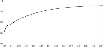
Figure 3. Projection of the generosity ratio (average pension/GDP per employed worker).
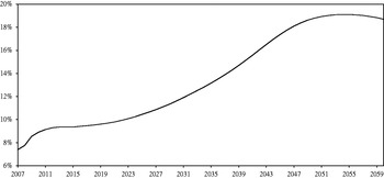
Figure 4. Projection of pension expenditure as a percentage of GDP.
We have also projected the evolution of the system's revenues and the balance of the Pension Reserve Fund (PRF) over the period of interest. Since Social Security contributions are levied at a fixed rate on wage income (subject to a ceiling and a cap), it seems reasonable to assume that as a first approximation, contribution revenue will remain constant over time as a fraction of the aggregate wage bill and of GDP. Starting from this assumption, we have introduced a minor correction to account for the increased State contribution to the financing of minimum pension complements that is mandated by law (see Appendix 1). With this correction, we project the pension system's revenues as a fraction of GDP to rise from 9.12% in 2010 to 9.52% in 2017 and to remain constant at that level thereafter. Under these assumptions, which are relatively optimistic, the system would experience a permanent deficit from 2019 onward. If we assume that the minor surpluses accumulated during some of the earlier years are deposited in the PRF and that this Fund earns a real annual return of 2%, the PRF would run out in 2027. After this point, the system's debt would balloon in the absence of policy changes, reaching 250% of GDP in 2060 (again assuming a real rate of return of 2%).
5 The financial effects of the reform: a quick estimate
The impact of the measures described in section 2 on the number of pensions per employed worker is easily calculated with a few additional assumptions. Increasing the retirement age will reduce the number of pensioners and increase the number of employed persons. To quantify the effects of this measure, we have ignored the possibility of early retirement and assumed that those affected by the increase in the retirement age have an employment rate that is similar to that of the population aged between 60 and 64 years in the year 2007 (which was 33%). In order to account for the exceptions to the raising of the retirement age, we will assume that only half of the potentially relevant population is actually affected by this measure.
Figure 5 shows the implications of the reform for the evolution of employment and the retirement-age population and Figure 6 summarizes its estimated impact on the number of pensions per employed worker. Under our hypotheses, the gradual rise in the retirement age will temporarily stabilize the ratio between pensioners and employed persons. Starting in the second half of the next decade; however, growth in the first variable surges, with dramatic effects on the first major component of pension expenditure.

Figure 5. Projection of employment and retirement-age population, with and without reform (2007 = 100).

Figure 6. Projection of the number of pensions per employed worker.
Projecting the evolution of the generosity ratio is somewhat more complicated than in the baseline scenario because of the gradual nature of the reform. For each transition year t we have used the model outlined above to calculate the long-term generosity ratio  $\bar{y}_{t} $ that would correspond to the parameters of the system at t, which would vary from year to year between 2012 and 2027. Figure 7 shows the time path of $\bar{y}_{t} $, which would gradually fall from 0.196 to 0.168 with the implementation of the reforms. Hence, the changes in the calculation procedure introduced in the new law will reduce the average pension (relative to the average wage) by 14.5% for a given time path of earnings and social contributions.Footnote 16
Figure 7. Evolution of the long-term generosity ratio with and without the reform.
To approximate the system's year to year dynamics, we will proceed as above while allowing the steady state to vary over time. That is, we will assume that in year t the value of the logarithm of the generosity ratio converges to its steady-state value for the same year and does so at the same rate we used in the previous section, in accordance with the following expression
 $$\rmDelta y_{t} \equals \minus b\lpar y_{t} \minus \bar{y}_{t} \rpar $$
which is identical to equation (7) except that $\bar{y}_{t} $ now has a time index that tells us that the system is approaching a moving target during the transition period.
Figure 8 shows the estimated trajectory of the generosity ratio after the reform. Combining this projection with our prior estimate of the number of pensions per employed worker yields the spending projection summarized in Figure 9 and the estimate of savings arising from the reform that is shown in Figure 10 as a percentage of GDP and measured in Figure 11 by the percentage reduction in pension expenditure. Figure 10 also shows our estimate of how savings would have increased in the absence of the noted exceptions to the new retirement age and Figure 11 shows a decomposition of the reduction in expenditure into its three immediate sources.Footnote 17 Looking at the last figure we see that in the long run the bulk of the expected savings come from the reduction in the generosity of the system, whose effects build up gradually over time and converge asymptotically to the 14.5% steady-state reduction in this variable estimated above. The reduction in the number of retirees is also important during the transition years but gradually loses importance once the age of retirement stops rising. Finally, the expected increase in employment is too small to have a significant effect on the spending ratio.
Figure 8. Projection of the generosity ratio of the pension system (average pension/GDP per employed worker) with and without the reform.

Figure 9. Projection of pension expenditure as a percentage of GDP, with and without the reform.
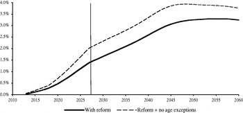
Figure 10. Savings resulting from the reform, in percentage points of GDP.
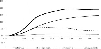
Figure 11. Percentage reduction in pension expenditure as a result of the reform and its immediate sources.
On the basis of our assumptions regarding the evolution of employment, productivity and demographics, the results of the analysis suggest that the proposed reforms would reduce pension expenditure by up to 20% by 2050. Expected savings would amount to 1.4 points of GDP at the end of the transition period in 2027 and to 3.25 points by mid-century (which would increase to 2.0 and 3.8 points, respectively, without the approved exceptions to the new retirement age). In this scenario, the reform would suffice to stabilize pension expenditure as a percentage of GDP during the transition period. In the absence of further reforms, however, spending is projected to rise quickly starting in 2030 and to reach 15% of GDP by 2050, thereby generating deficit levels that would be very difficult to sustain.
The implications of the reform for the financial balance of the system are summarized in Figure 12, which displays the expected evolution of the PRF or the system's accumulated debt with and without the reform. As noted above, in the no-reform scenario, the PRF would run out by 2027. The reform would push this date back to 2037, giving us an additional decade to design and implement the additional measures that would be required to prevent the insolvency of the system during the 2040s. Eliminating the exceptions to the new retirement age would buy us five additional years before the PRF runs out.
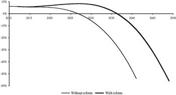
Figure 12. Projection of the PRF/accumulated debt of the pension system as a percentage of GDP.
Comparison with other projections
A number of other estimates of the effects of the recent reform are already available. The Spanish Ministry of Economics and Finance has included its own projections (with and without taking into account the so-called sustainability factor) in the latest version of Spain's Stability Program for 2011–14 (MEH, 2011). These projections seem to have been accepted by the OECD and the IMF and have been included in their recent reports on pension systems in member states and on the situation of the Spanish economy (OECD, 2011; IMF, 2011). The Ministry, however, gives few methodological details and reports only that its estimates have been based on INE's (2010) demographic projections and on a macro scenario consistent with the common methodology used by EU members for medium- and long-term projections. The Bank of Spain has also included estimates of the savings derived from the reform in its recent annual report (2011), which have been obtained using an overlapping generation model and Eurostat's 2008 population projections. Some academic researchers have also studied the subject. Conde-Ruiz and Gonzalez (Reference Conde-Ruiz and González2011) analyze the effects of the reform using an accounting model with heterogeneous agents calibrated using data from the Labor Force Survey and the Continuous Sample of Working Lives and INE's (2005) long-term population projections. Finally, Díaz-Giménez and Díaz-Saavedra (Reference Díaz-Gimenez and Díaz-Saavedra2011) use a calibrated dynamic general equilibrium model and INE's 2010 population scenario to analyze the impact of two of the three key measures introduced in the recent law: an increase of two years in the retirement age and the extension of the calculation period from 15 to 25 years. Table 3 compares our estimates of the savings arising from the reform with those from other studies. As can be seen in Table 3, our results lie almost exactly in the middle of the range of the available estimates when savings are measured in relative terms (as a fraction of the expected increase in pension expenditure in the absence of the reform) and at its upper end when savings are measured in absolute terms (as percentage points of GDP). While there are significant differences across estimates that are not always easy to trace back to primary assumptions (because of the use of very different approaches and the limited methodological information that is provided in some cases) all the existing studies agree in qualitative terms and suggest that the recent reform will significantly reduce the growth rate of pension expenditure over the next four decades.
Table 3. Alternative estimates of the savings derived from the reform
Note: The second column is obtained by dividing the first one by the expected increase in pension expenditure in the absence of the reform until 2050. In the case of MEH (2011) and Bank of Spain (2011) this last magnitude is taken from the official estimates of aging-related expenditure prepared by the Economic Policy Committee of the EU. In our case and that of Conde and González (Reference Conde-Ruiz and González2011) we calculate it as the difference between projected expenditure in 2050 and observed expenditure in 2010 and in Díaz Giménez and Díaz Saavedra as the difference between projected expenditure in 2050 and in 2010.
6 Conclusions
This paper presents a preliminary estimate of the financial impact of the recent reform of the Spanish public pension system. After updating our earlier projections of spending on contributory pensions during the period 2008–60 in the absence of reforms (de la Fuente and Doménech, Reference de la Fuente, Doménech and Jimeno2010), we have estimated the impact on this variable of the three main measures included in the new law: increasing the retirement age to 67 years with significant exceptions, extending the pension calculation period to 25 years and increasing to 37 the number of contribution years required to be entitled to 100% of the regulatory base.
Although reasonable doubts remain as to whether or not these measures will be sufficient to ensure by themselves the financial sustainability of the system, they do constitute a significant step in the right direction for three reasons. First, because they have triggered an important public debate about the sustainability of the public pension system that has not been restricted to the political parties. Second, because the agreement to raise the retirement age has broken a real taboo. Now that that barrier has been crossed, it will be much easier to deal with further changes that may be required in the future to ensure the sustainability of the system. Lastly, and in line with the previous point, because the introduction of the sustainability factor entails a qualitative change in the nature of the system by introducing a quasi-automatic mechanism for making reforms that had previously required long gestation periods and laborious agreements.
Contingent upon certain assumptions about the evolution of employment, productivity and demographics, the results of this paper suggest that the three main reforms introduced in the new pension law will have a significant impact on expenditure and may be expected to yield savings of around 1.4 points of GDP at the end of the transition period in 2027 and of 3.25 points by mid-century. In this scenario, the reform would stabilize pension expenditure at a bit over 9% of GDP during the transition period, thereby preventing the emergence of a structural deficit in the system before the end of the next decade. In the absence of further reforms, however, we anticipate that expenditure will increase rapidly after 2030, reaching more than 15% of GDP by 2050. Hence, additional reforms will be required in the future to prevent the emergence of large deficits.
Given the uncertainty that surrounds the projections of many of the variables of interest, we cannot rule out the possibility that, even with the reform, the system may begin to experience a structural deficit before the end of the transition period. Under these conditions, a sensible precaution would be to move up the introduction of the sustainability factor to the start of the reform, rather than waiting for the end of the transition period. This would activate a mechanism that could be used to modulate the pace and scope of the reforms, should the financial situation of the system so require before the end of the transition period. Further, it is clear that the financial health of the system depends not only on the evolution of life expectancy but also on other variables such as the employment and dependency rates that influence the number of pensions per employed person. One important implication of this observation is that the sustainability factor cannot be linked only to life expectancy, as the wording of the law appears to indicate (BOE 2011, art. 8), but must also take into account other variables that are relevant to the financial health of the system.
In addition to any further parametric changes that should prove necessary in the future to ensure the sustainability of public pensions, it is very important to increase the transparency of the system by supplying additional information both to contributors and to pensioners. This would enable society to internalize the close relationship that exists between contributions and benefits and would help workers make timely and informed decisions regarding the best way to prepare for retirement. The experience of other European countries that have introduced models with notional accounts in their public pension systems, such as Sweden, Italy, Poland or Latvia, should provide a useful reference in this regard. While stopping well short of this mark, the new law does take an important preliminary step in the correct direction by requiring both the Social Security system and the operators of private pension plans to provide their contributors or participants with information regarding their likely future pension rights (additional disposition no. 26). The provision is, however, rather vague and it remains to be seen how it will be implemented.
Appendix 1. Data on pension revenues and expenditures
The expenditure data we use as a starting point for our calculations refer to spending on contributory pensions by the Spanish Social Security system. The Gazette of Labor Statistics (Boletín de Estadísticas Laborales) (MITIN, 2011a) provides data on the number of pensions paid every month (between 1988 and 2010) broken down by type of pension (retirement, disability, survivors' benefits, and benefits for orphans and other family members) and the average amount of each type of pension.Footnote 18 Total pension expenditure is estimated by multiplying the average number of pensions payable in each year by their average annual amount (which is calculated as 14 times the monthly amount).Footnote 19 The calculation is done separately for each type of pension and the results are aggregated. We have checked that the total obtained in this way approximately matches the figure in the General State Budget for this item.
In Spain, contributions for common contingencies cover a series of contingencies in addition to retirement. As a result, it is not possible in principle to isolate a specific contribution to the pension system. On the basis of an internal Spanish Government report cited by Doménech and Melguizo (Reference Doménech, Melguizo and Franco2008), we estimate that 95% of such contributions can be imputed to the pension system. To this, we must add a transfer from the State's General Administration to cover a growing fraction of the ‘minimum complements’ that raise the lowest contributory pensions to the minimum set by law. Our data on the system's revenues are taken from the Economic and Financial Report of the General Social Security Budget for fiscal year 2011 and the Appendix to that document (MITIN, 2011b).
According to MITIN (2011c, pp. 54 and 185) in 2010 the system's total revenues amounted to 9.12% of GDP. State contributions to minimum pension complements totaled 2.70635 million euros, or 0.25% of GDP, which represented 38.8% of the total cost of the program (of 6.97243 Meuros). The Social Security Law currently in force (transitory disposition no. 14 in BOE, various years) establishes that the State should pay the full cost of pension complements by 2014, but it is widely acknowledged that the current state of public finances will make it impossible to reach this goal on time.Footnote 20 Trying to be realistic, we have assumed that the State gradually increases its contribution to the programme starting in 2013 and starts covering its full cost (which is assumed to remain constant as a percentage of GDP) by the year 2017.
Appendix 2. Europop 2008 versus Europop 2010
As noted in the text, Eurostat has recently updated its population projections for EU member countries. Table A1 and Figure A1 compare the basic assumptions underlying the two Europop projections. Europop 2010 is a bit more optimistic than its predecessor regarding the evolution of life expectancy of both males and females and assumes a rather different time path of net migration inflows. In view of the sharp decline in inmigration observed during recent years as a result of the current crisis, the time path of migration assumed in Europop 2010 seems more plausible than that projected in the earlier exercise. In spite of this, average yearly inflows are almost identical in the two scenarios.
Figure A1. Net inmigration projections, Europop 2008 vs. 2010.
Figure A2. Projections of the old-age dependency ratio, Europop 2008 vs. 2010.
Table A1. Assumed values of key demographic parameters in 2060
The difference in migration profiles has the expected effect on the time path of the dependency rate (defined here as the ratio between the population aged 65 years or more and the population between 15 and 64 years of age). Since inmigration is slower in the Europop 2010 scenario during the first half of the period and faster during the second half, the dependency ratio rises faster at first and then falls below the path expected in the previous exercise. The effect of this on the net financial balance and on the pension system is straightforward. Other things equal, switching from Europop 2008 to Europop 2010 will bring the system into deficit at a somewhat earlier date but will also modestly reduce the severity of its financial problems in the final part of the sample period (Figure A2). It should be emphasized, however, that the results of the exercises undertaken in this paper would not change qualitatively with the adoption of the new Eurostat projections as our starting point.


