1. Data

We use harmonized data provided by the Gateway for our analysis, and supplement it with individual elements from each survey's original data.Footnote ⁵ Using the HRS, we assess the validity of alternative approaches for computing prospective public pension benefits. Then, using both the HRS and the English Longitudinal Study of Ageing (ELSA), we evaluate whether the relationship between retirement decisions and pension benefits and benefit growth levels computed using our survey-based approaches are consistent with income and substitution effects. Both the HRS (1992–present) and ELSA (2002–present) benefit from long panels, so we can use our prospective benefit measures to look at behavior a decade later.

The HRS started in 1992 with 12,652 respondents from households where at least one member was born between 1931 and 1941, re-interviewing these respondents biannually. The HRS has expanded over time and now encompasses more than 30,000 respondents and represents the US population over the age of 50.Footnote ⁶ Importantly for this paper, the HRS has negotiated with the Social Security Administration to link survey data with the administrative data on covered earnings back to 1951 and records on benefit claiming, entitlements (after claiming the benefits), and payments.

The ELSA started in 2002, now surveys over 12,000 respondents biannually, and is representative of the English population aged 50 and over (Banks et al., Reference Banks, Blake, Clemens, Marmot, Nazroo, Oldfield, Oskala, Phelps, Rogers and Steptoe2018). ELSA does not link respondents with their administrative earnings and public pension records. However, it collects retrospective life-history data, including the start and end year of jobs lasting at least 6 months, starting salary of those jobs, and final salary at the last career job.

2. Estimating prospective benefit levels

Ideally, each longitudinal survey would be linked with administrative data on work and earnings histories as well as public pension benefits. Alternatively, some HRS-sister surveys have collected retrospective work histories that provide a portion of information needed to compute prospective pension benefits. In this section, we evaluate five approaches applied to HRS data by computing a ratio of the benefit predicted by each approach to the benefit actually observed in the administrative data.

In conducting our analysis using HRS data, we restrict the sample to individuals who (1) are observed working full-time at an interview before claiming their Social Security old-age benefit and who are observed after they have claimed their Social Security benefit, (2) have authorized their Social Security data to be linked with the HRS survey, and (3) do not initially claim auxiliary benefits, such as spouse and survivor benefits (although we still include individuals that eventually claim survivor benefits). The first restriction will limit the sample to individuals who are working late in life. We expect the second restriction to have limited influence on our analysis. Analysis by Haider et al. (Reference Haider and Solon2000) indicates that 75% of individuals in the 1992 HRS cohort authorized their Social Security data to be linked to their HRS survey responses and that this authorization was generally unrelated to most of the respondent's observable characteristics, with minor differences by race and for individuals with nonexistent work histories. The final restriction to individuals who do not initially claim spouse and survivor benefits will omit individuals with limited earnings history, particularly women. We view these restrictions as reasonable because the purpose of this section is to validate the accuracy of our approaches for computing prospective pension benefits for those who have not retired and for whom claiming benefits is meaningful for their decision to work.

3. Five approaches for predicting pension benefits

We consider five approaches to predict each respondent's pension entitlement, which is not known because of incomplete information. Most public pension benefits are determined by past earning and contributions, and claiming history. We provide evidence on the tradeoffs between accuracy, precision, and data requirements in each approach.

Approach #1 (A1) takes the last observed income at a full-time job prior to benefit claiming, treats this income level as the individual's average lifetime earnings for computing the benefit level, and uses the pension rules to compute their retirement income assuming a full career. We define a full career as working every year from entry into the labor force (the greater of 18 or years of education plus 6) until the age at the last interview where the respondent is working full-time.

Approach #2 (A2) follows a similar process to A1, except that the average lifetime earnings measure in the pension formula uses gender-specific earnings trajectories by work experience estimated using the approach described in Lagakos et al. (Reference Lagakos, Moll, Porzio, Qian and Schoellman2017) with data from the 2003–2016 American Community Survey (Ruggles et al., Reference Ruggles, Flood, Goeken, Grover, Meyer, Pacas and Sobek2018). Like Lagakos et al. (Reference Lagakos, Moll, Porzio, Qian and Schoellman2017), our model of earnings trajectories controls for education, cohort, and time effects, reflecting only differences in earnings by work experience. Our estimates exhibit greater lifecycle earnings growth relative to what is reported in Lagakos et al. (Reference Lagakos, Moll, Porzio, Qian and Schoellman2017).

In Figure 1, we compare our earnings trajectories based on potential experience to median earning trajectories for individuals with at least 35 years of earnings in the administrative data (all earnings trajectories are computed relative to earnings in the last year of full-time work). We find remarkably similar trajectories for men, however divergent trajectories for women. The dichotomy in the earnings trajectory for women may reflect volatility in their work experience (e.g., leaving one career when they have children and starting a new career after their children are in school).

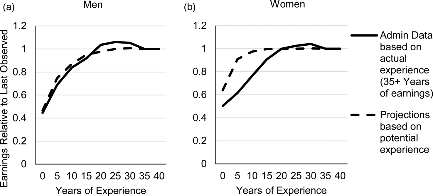
Figure 1. Comparison between imputed earnings trajectory and median earnings trajectory based on administrative data.

Note: Author's calculations using HRS data linked to SSA data on earnings histories. Earnings are measured relative to earnings in the last year of experience (e.g., if an individual had constant real earnings, then his earnings trajectory would be flat and equal to 1). Sample sizes of individuals with 35+ years of actual experience in the administrative data are 1,130 for men and 336 for women.

Men with at least 30 years of earnings history, representing 90% of the sample, exhibit, on average, earnings trajectories that grow over the lifecycle, whereas individuals with less than 30 years of experience exhibit flatter earnings trajectories. The flatter earnings trajectories may reflect that individuals with limited or sporadic work histories do not accumulate specific-human capital that leads to wage growth over the life-cycle. This demonstrates the importance of work history data in determining earnings trajectories. The next two approaches consider how incorporating information on work history might influence the benefit predictions.

Approach #3 (A3) adds to the approach in A2 by reflecting variation in work experience based on a lower bound for work experience imputed from responses to questions on past employment asked during the first interview. Respondents are asked about their tenure at a current job or at their most recent job if not currently working. Additionally, they are asked for the number of jobs where they worked at least 5 years. Only for the most recent of those past jobs was retrospective information collected, and only if that job occurred within 20 years of the interview. We combine these questions to produce a minimum value for work experience as of the respondent's first interview.

We classify individuals as having sporadic work histories if they are likely to have less than 30 years of earnings.Footnote ⁷ For those with sporadic work histories, A3 follows the approach in A1 and assumes a constant real earnings trajectory over the lifecycle. This reflects the median profiles for individuals with less than 30 years of non-zero earnings in the administrative data. For individuals with non-sporadic earnings trajectories, A3 predictions use the earnings trajectories in A2.

A number of HRS-sister studies have collected retrospective work histories, which are more comprehensive than questions asking about past employment collected during the first interview.Footnote ⁸ In lieu of a work-history module in the HRS, approach #4 (A4) approximates the information provided by a work-history module by treating person-year records with non-zero earnings in the administrative data as a proxy for full-time work.Footnote ⁹ We expect A4 to be more accurate than the measure in A3 because more information is used (e.g., start and end date, full-time status). A4 predictions use the earnings trajectories from A2, but lifetime earnings reflect the actual years worked from the work-history module.

Approach #5 (A5) replaces respondent reported earnings with the actual administrative earnings history.

A1 reflects the most naïve approach, not incorporating lifecycle wage growth or variable work histories. A2 refines this approach by accounting for average lifecycle wage growth, and A3 and A4 further refine that approach by accounting for variable work history. A1–A4 demonstrate how introducing coarse pieces of survey information (e.g., last reported earnings and years of work experience) and combining it with projected earnings trajectories can improve the accuracy of prospective pension benefit predictions. Since public pension systems often have many minor rules that influence actual benefit levels, A5 is used to demonstrate how accurate our benefit formula is given the administrative data on earnings history. If the administrative earnings and benefit data are accurate and the benefit formula restricted to only those elements we model (earnings and contribution history conditional on claiming age) represents the only important factors for determining benefit levels, then A5 would provide a precise measure of the realized benefit levels.

In light of the discrepancy between our computed and observed earnings trajectory for women noted in Figure 1, we do not include women in our validation analysis, as it is likely that the predicted pension benefit levels will be notably biased upward for A1–A4.

4. Validation of approaches to predicting benefit levels

SSA administrative data reports the monthly benefit amount (MBA). It reflects the benefits an individual is entitled to based on his or her earnings history and benefit claiming age, incorporates reductions for collecting benefits before the full retirement age and delayed retirement benefits for retirement after that age.Footnote ¹⁰ Additionally, MBA will reflect adjustments based on military service, for work after claiming, or reductions due to receipt of non-covered public pensions. These adjustments are specific to the US public pension and reflect additional complexities not captured in our computation of US public pension benefits.

We compute prospective Social Security benefits $(\widehat{{MBA}})$ using the following formula:

$$\eqalign{& \widehat{{MBA}} = CF \times PIA \cr & PIA = 0.9 \times \min (AIME,BP1) + 0.32 \times {\rm max(min(}AIME-BP1,BP2{\rm )},0{\rm )} \cr &\qquad\,\,\, + 0.15 \times {\rm max(}AIME-BP2,0{\rm )}} $$

where CF reflects that adjustment factor based on claiming age, PIA reflects the primary insurance amount, BP1 and BP2 reflect the first and second bend points that are based on an individual's birth year, and AIME reflects the person's best 35 years of indexed monthly earnings where earnings before age 62 are adjusted for average wage growth over time.

In the remainder of this subsection, we consider two questions:

1. (1) Do our approaches do a reasonable job of approximating MBA in terms of average and individual benefit levels?

2. (2) Do our survey-based approaches (A1–A4) result in the same benefit levels as our administrative data approach (A5)?

We will assess the ability of the approaches to capture MBA by computing the ratio of the prospective benefit level to the MBA. Bias will be reflected in mean and median differing from one, and precision will be reflected by the standard deviation.

Figure 2 provides a cumulative distribution of the ratio between A1 and A4 approaches and the administratively reported benefit entitlement (i.e., $\widehat{{MBA}}/MBA$), and Table 1 provides additional information about the distributions. Ideally, this ratio would be equal to one, implying the predicted benefit from our approaches would be equal to the administrative report of the benefit entitlement.

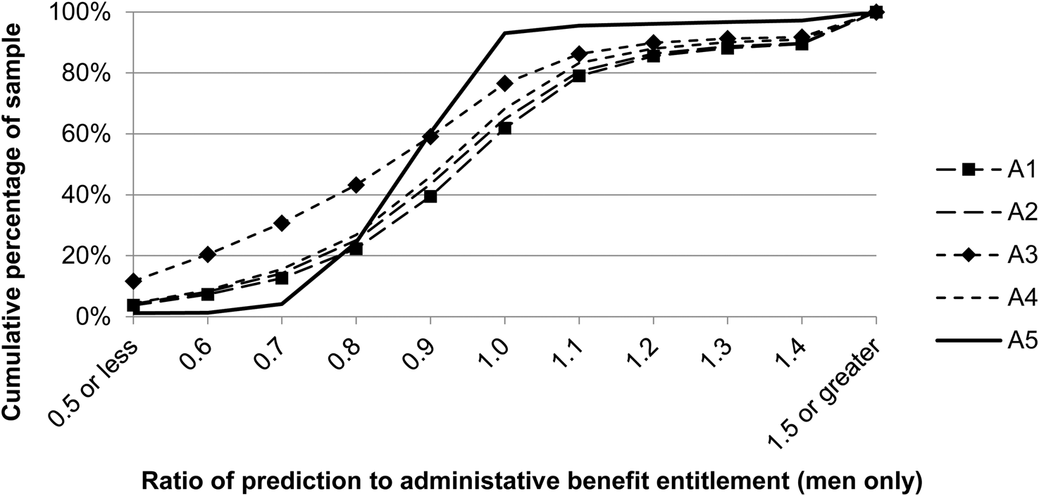
Figure 2. Cumulative distribution of ratios for predictive approaches to administrative reports (men only). Note: Author's calculations using HRS data linked to SSA data on earnings histories and benefit entitlements. The sample is unweighted and only includes respondents observed working full-time before their self-reported claiming age and for whom we are able to compute benefit levels for every approach. The correlation in the last column reflects the computation of a Pearson correlation coefficient between the $\widehat{{MBA}}_X/MBA\; $ for X = A1 to A4 with $\widehat{{MBA}}_{{\rm A}5}/MBA$. X-axis values represent the range of ratios from the value referenced up to, but excluding, the next value (e.g., 1 = [1.0,1.1]).

Table 1. Summary statistics of ratios for predictive approaches to administrative reports (men only)

Note: Author's calculations using HRS data linked to SSA data on earnings histories and benefit entitlements. The sample is unweighted and only includes respondents observed working full-time before their self-reported claiming age and for whom we are able to compute benefit levels for every approach.

A1–A4 provide upward biased predictions of benefit entitlements with a right skew (reflected in 8–10% with predicted benefit levels with a ratio of 1.4+ relative to actual entitlement). This is not unexpected for A1 and A2 that assume 35+ years of full-time earnings experience. The skewness results in the mean exceeding the median, although the median is generally closer to one (Table 1). A3 stands out as substantially underpredicting relative to actual entitlements for a larger fraction of the sample (e.g., 43% of the benefits predicted using this approach reflect 80% or less of the true entitlement). Stepwise, adding information in the approaches A2–A5 results in a decline in the standard deviation, an improvement in precision of the estimates. Hence, accounting for work history and earnings trajectory improves the fit of prospective benefits for men. The improvements between A1 and A2 are surprisingly limited. A3 and A4 reduce the bias, but substantial variation persists. A5 still exhibits variation relative to the administrative benefit amount, albeit significantly closer (the standard deviation is 0.21 compared with 1.00 or greater for other approaches).

Since Table 1 indicates the approach using administrative earnings histories (A5) is both precise and relatively free of bias, we will subsequently refer to it as a benchmark for the ‘true’ benefit levels and incentives that we model. Table 2 reports the correlation between the alternative approaches and A5 showing that the correlation is reasonably high (i.e., that low beneficiaries in one approach are low beneficiaries in the other). For example, 28% of the variance in A5 can be explained by A1, and this rises to 36% for A4.Footnote ¹¹

Table 2. Correlation between survey-based approaches and the administrative data approach for predicting benefit levels (men only)

Note: Author's calculations using HRS data linked to SSA data on earnings histories. The sample is unweighted and only includes respondents observed working full-time before their self-reported claiming age and for whom we are able to compute benefit levels for every approach. The correlation reflects the computation of a Pearson correlation coefficient between each survey-based approach for computing benefit levels and A5. The benefit growth level is computed by computing the growth in benefits from an individual working an additional year and delaying claiming if necessary (see paper for a discussion), and the benefit growth rate is computed by dividing the growth level by the original benefit level.

We conclude that our survey-based approaches broadly capture MBA on average, but they exhibit a positive bias and non-trivial error. Our efforts to reduce bias by accounting for lifecycle trajectory in earnings result in limited improvements in bias and precision. Incorporating work history, particularly one that reflects stops and starts that are observed in the administrative data, leads to seemingly minor reductions in bias but improvements in precision. Simply knowing the individual's report of his last full-time earnings explains about 28% of the variation in the final benefit level, with the only substantial improvement arising from a detailed work history which can explain 36% of the variation (i.e., A4). The remaining variation is then attributable to volatility in earnings over the lifecycle and reporting error, the latter of which can come in a variety of forms including incorrectly reported final earnings.

What are the implications of these conclusions? Given the progressivity of pensions, the positive bias in benefit levels will likely lead to a negative bias in the predicted benefit growth, a point we will explore next. This negative bias in benefit growth will persist regardless of the approach because the positive bias in the benefit levels is persistent. Imprecision and residual unexplained variation will lead to measurement error, a subject we will return to in the final subsection. Finally, since including work history provides limited improvement in precision, we expect that the use of work histories will not substantially mitigate the negative effects of measurement error on predicted benefit levels.

5. Projecting benefit growth using alternative approaches for predicting benefits

In this section, we project individual benefit growth for working an additional year. We compare how projections using four approaches that rely on commonly collected survey data differ from an approach using administrative data on earnings histories (i.e., A5). The difference reflects the role of earnings history (dynamics and lifetime level) for determining the magnitude of annual benefit growth from an additional year of work and delayed claiming. We consider two questions:

1. (1) For the approaches based on survey data, do we observe a negative bias in the estimated benefit growth?

2. (2) Do the approaches relying on survey data capture the same benefit growth as that implied by the administrative data?

We address the first question by comparing the distribution of approaches relying on survey data to the distribution of A5. For the last question, we compute the correlation between the computed benefit growth for each of the different approaches. Benefit growth rates, even if biased, can still be used to identify relationships with an outcome of interest if they are highly correlated (e.g., do greater pension benefit growth rates encourage continued work?).

For our computation of benefit growth, we assume that if an individual works an additional year, he will receive the same real wage as he earned in his last year of work (consistent with the earnings profiles in Figure 1). For individuals at or above the eligibility age, we assume that they delay claiming of their Social Security benefit for that year.

Figure 3 depicts the cumulative distribution of benefit growth rates from working for one more year. We observe sharp increases at 0 and 8% for A5 (i.e., greater than 10% of the sample). The first increase would correspond to individuals who were under the age of 62 or over the age of 70, for whom working an additional year would only increase benefits if the additional year of earnings resulted in an increase in their AIME. The increase at 8% likely corresponds to individuals between early retirement age and age 70 where the benefit to delaying claiming (independent of the AIME) is 6.7–8.3% before the normal retirement age and 3.0 to 8.0% after. As noted in the last section, the positive bias in the computed benefit levels across A1 to A4 should result in negative bias in benefit growth. Indeed, Figure 3 shows that this is true for A1, A2, and A4. A3 stands out relative to A5 as reflecting generally higher benefit growth rates relative to A5 (as represented by the cumulative distribution being everywhere lower than A5 in Figure 3). Recall that A3 uses a ‘minimum years worked’ measure. The effect of this is an incomplete earnings history, meaning that AIME typically reflects fewer than 35 years of earnings, which means an additional year of earnings can have a large effect on the base benefit level.

Figure 3. Cumulative distribution of benefit growth from working one additional year (men only).

Note: Author's calculations using HRS data linked to SSA data on earnings histories. The sample is unweighted and only includes respondents observed working full-time before their self-reported claiming age and for whom we are able to compute benefit levels for every approach. We assume real earnings from an additional year of work are the same as the last year worked full-time and individuals eligible to claim benefits choose to delay claiming them while working. X-axis values represent the range of benefit growth rates from the value referenced up to, but excluding, the next value (e.g., 0% = [0,1]).

We compute correlations of individual benefit growth levels and rates (percentage change in benefit level) between the survey data-based approaches and A5 (reported in Table 2). We find that the survey-based approaches are remarkably highly correlated (ranging from 0.83 to 0.94) with the administrative-data approach. This implies that regardless of the approach, our benefit growth measures largely reflect the true marginal incentives to postpone retirement despite the survey-based approaches being less successful in predicting benefit levels. This suggests that, given the nature of the benefit rules, the change in benefit levels from working an additional year is largely reflected in factors observed in the surveys and common to all approaches, such as earnings at last full-time job and age.Footnote ¹²

We conclude that approaches A1, A2, and A4 result in negatively biased growth rates. If the present value of pension benefits are computed using these approaches, then measurements intending to capture financial incentives to postpone the retirement will also exhibit this same bias. These include accrual, peak, and option value measures (Gruber et al., Reference Gruber and Wise2004). On the other hand, A3 exhibits the opposite pattern, given its assumption of a lower bound on career length. All of the approaches provide a strong instrument for true benefit growth resulting from postponing retirement.

7. Demonstration of relationship between predicted benefits and retirement behavior

Theoretically, all else equal, individuals entitled to greater pensions should be more likely to retire (income effect). Additionally, individuals that would see larger growth in their pension benefit from working another year should be more willing to delay retirement (substitution effect). If these aspects of the pension's design are salient in the retirement decision, then the benefit and benefit growth levels should reflect incentives, all else equal. The predicted pension benefit and the predicted benefit growth if postponing retirement by 1 year represent our best approximations using commonly available data and methods that can be employed across the HRS-sister surveys in lieu of administrative data. In this section, we apply our approaches to HRS and ELSA data. We limit our analysis to men in 2004 that are between ages 53 and 61.Footnote ¹³ First, we introduce key attributes of the UK pension system and how we apply them to the ELSA data. Second, we provide descriptive statistics for the USA and England in 2004, and in the final section, we evaluate whether the relationship between retirement decisions and both current pension entitlements and the change in these entitlements if postponing retirement by 1 year are consistent with the income and substitution effects.

8. UK pension structure

We focus on the UK pension system between 2004 and 2014 for male workers.Footnote ¹⁴ There are three key components to the UK public pension system: Basic State Pension (BSP), Additional State Pension (AP), and earnings-based second pension, and the pension credit (PC), a means-tested benefit.Footnote ¹⁵ In addition to the public pension system, many employers offer occupational pensions. The pension law in effect between 2004 and 2014 allowed individuals to opt out of the earnings-related pension, effectively reducing (but not eliminating) their contribution to the UK public pension system. The state pension age for men is 65. Individuals could not claim their pensions before age 65 but they were provided an additive annual increase of about 7.4% for each year delayed between ages 65 and 70 prior to 2005 and an additive annual increase of 10.4% starting in 2005.

BSP is based on a fixed rate (e.g., £79.60 per week in 2004). Individuals must have at least one qualifying year of contributions to the UK National Insurance system to be eligible for the BSP. For individuals with less than 44 qualifying years, benefits are reduced by 1/44th per year. From 1980 to 2003, the weekly benefit rate was increased in line with prices. Since 2003, the government's policy has been to increase the state pension by at least 2.5%, regardless of the level of inflation (Bozio et al., Reference Bozio, Crawford and Tetlow2010).

The AP reflects two state pension schemes based on earnings: (1) State Earnings-Related Pension Scheme (SERPS), 1978–2002, and (2) the State Second Pension (S2P), 2002–2015. S2P will reflect the pension incentives relevant for our sample. The formula for AP is included in online Appendix B. In computing prospective pension benefits, we include the aspects of the formula that reflect work and earnings history under SERPS and S2P, the applicable minimum and maximum earnings that contribute toward the AP, and the incentives to delay claiming (as with BSP, men cannot claim AP before age 65). The final aspect of the UK public pension is the PC, which provides an income floor for all individuals. We do not incorporate it into our analysis as it is a universal benefit.

9. Cross-national descriptive statistics

Table 3 presents the sample statistics for our English and US samples of working men. The first column for each country presents the sample prior to restricting it to men working full-time in 2004 and response in later interviews. In England, we find that about 82% are married, and around 20% have at least a college education. The average household consists of 2.4 people on average. Those working full-time are more likely to be married, have at least a college degree, earn more while working, and have accumulated fewer assets as of 2004. Number of people in the household and the number of children are the same on average between the overall sample and the sample restricted to those working full-time in 2004. These patterns are similar for the USA, except individuals working full-time in 2004 generally having greater assets. More generally, US men ages 53–61 in 2004 were less likely to be currently married.

Table 3. Descriptive statistics

Note: Authors’ calculations using HRS data and the 2004 person-level weights for each survey. The sample is restricted to men with non-zero sample weights that are between the ages of 53 and 61 in 2004. Monetary values reported in 2010 levels of the local currency. The 2010 annual average of the US dollar to UK pound sterling exchange rate was 0.65.

10. Relationship between predicted benefits and retirement behavior

We evaluate whether the relationships between retirement decisions and pension benefits and benefit growth levels computed using our survey-based approaches are consistent with the income and substitution effects. We estimate a probit model of retirement in 2014 for men who were working full-time and were between the ages of 53 and 61 in 2004. Our factors of interest are the coefficients on individual i’s benefit level at time t (benefit _i,t) and the growth in his benefit if he works and delays claiming for 10 years (growth _i,t,t+k = benefit _i,t+k − benefit _i,t). The model is:

$$Retire_{i,t + 10} = {\rm Pr}\left( {\beta_0 + \beta_1growth_{i,t,t + k} + \beta_2benefit_{i,t} + \mathop \sum \limits_{\,j = 54}^{61} \beta_{3,j}age_{i,t}( j ) + \beta_4X_{i,t} + \varepsilon_t > 0} \right)$$

where we are testing if β ₁ < 0, β ₂ > 0. The variable age _i,t(j) represents an indicator taking a value of one if individual i is age j in year t, and X _i,t is a vector of controls unrelated to the individual's own public pension benefit level and growth rate, such as reported assets and marital status. We do not include income, as our predictive approaches generally rely on final income to predict the benefit level, and as such are highly collinear.Footnote ¹⁶ Table 4 presents the results for the four survey-based approaches in England and USA, and the approach using administrative data in the USA.

Table 4. Probit models of not working full-time in 2014 conditional on working full-time in 2004

Note: Authors’ calculations from estimating probit models using HRS data, robust standard errors, and the 2004 person-level weights for each survey. Marginal estimates are reported for the explanatory factors. For brevity, age dummies are omitted from the table. Standard errors for the marginal estimates are calculated using the delta method and are denoted with parentheses. Monetary values are reported in 2010 levels of the local currency. The 2010 annual average of the US dollar to UK pound sterling exchange rate was 0.65. In the UK, we exclude individuals with full-time earnings in 2004 below the 2010 lower earnings threshold (£110 per week), as these individuals would be eligible for the means-tested benefit. Sample sizes otherwise differ from Table 3 due to an inability to predict pension benefits based on survey responses.

With one exception, the estimated coefficients are consistent with the income effect (positive coefficient on benefit level) and the substitution effect (negative coefficient on benefit growth levels) but are not always statistically significant. Comparing the English to the US point estimates for benefit growth levels, an additional $1,000 (equivalently £650) in pension benefits from continuing to work until 2014 is associated with a 2–3 percentage point lower likelihood of retiring by 2014 in England, and 2–4 percentage points in the USA. The lack of significance in Table 4 should not necessarily be construed to be an indication that the survey-based approaches are poor indicators. US benefits computed using A5 should be a strong instrument for true benefit levels and benefit growth levels. Using this approach, benefit growth is significant while the benefit level is not significant. This insignificance of the point estimate may result from benefit levels not consistently being a meaningful determinant of retirement over this timeframe, although it may be more salient for specific groups (e.g., those without other sources of retirement income).

Reflecting on the implications of our analysis of the approaches, we expect the benefit growth levels using A1, A2, and A4 to be negatively biased, suggesting that if the growth in the pension level from 2004 to 2014 were related to retirement in 2014, the coefficient point estimates should be biased away from zero. This is the case for each of these approaches when compared with A5.

Benefit growth between 2004 and 2014 is more consistently associated with retirement in 2014 (as measured by the significance of the coefficients) in the USA rather than England. This could reflect other policy characteristics associated with the UK that may dominate public pension incentives (e.g., age 65 is a common private pension age in England), independence of work and delayed claiming incentives (i.e., there is no earnings test in the UK), reflect non-salience of UK pension rules, or simply smaller sample sizes.

In summary, we find that our measures of prospective public pension benefits created with our survey-based approaches perform consistent with our hypotheses when placed in a simple model of retirement. A key takeaway is that pension benefit growth measures using relatively naïve approaches seem to perform in a manner yielding results that are consistent with more sophisticated measures, including approaches accounting for work history or administrative earnings history. We expect this to be true in circumstances where (1) pension benefits are based primarily on lifetime earnings and the individuals under study have long working lives, and (2) significant incentives, penalties or prohibitions for benefit collection are part of the benefit design (e.g., large delayed retirement credits – as in the USA and UK; earnings test for benefit receipt – USA).

Our measures assume individuals claim their benefits when they retire from full-time employment or when they are first eligible, which is a common assumption in papers on pension incentives. If an individual does not follow this pattern (e.g., stops working but does not claim his benefit), then he could increase his lifetime benefit without altering his work behavior. A study aimed at understanding claiming incentives independent of work incentives would require a prospective benefit measure that does not link claiming and work.

Ultimately, the ideal measure depends on the research question. Our analysis reveals that the factors contributing to pension incentives vary in magnitude, suggesting that a simpler measure may be sufficient to identify the relationship between financial incentives to retire and outcomes of interest.