1 Introduction
In recent years, many countries have reformed their public pension system, tightening the eligibility rules and reducing the generosity of benefits (Feldstein and Siebert, Reference Feldstein and Siebert2002). Partly as a result, private pension plans have grown in terms both of assets under management and of number of participants (OECD, 2009), becoming increasingly relevant as a means to provide adequate retirement income.
Contrary to Social Security schemes, private pension investment requires the worker to make several choices. She has to decide whether and how much to contribute, select the most appropriate portfolio, and possibly decide when to withdraw. These decisions are even more difficult in a time of financial turmoil, when both the probability and the cost of errors are magnified. In order to design policies, which help workers to get the most out of their pension investments, it is important to understand how their behaviour is systematically affected by individual characteristics such as age, sex, financial education and income.
In particular, the aim of the present paper is to assess the effect of age on portfolio choices, using a new panel dataset from a defined-contribution (DC) pension plan for employees of a medium-size Italian bank.
Recent optimal portfolio theories suggest that investors should reduce their exposure to stock market risk as they get near to retirement (see, e.g., Campbell and Viceira, Reference Campbell and Viceira2002), and failure to do so can be quite costly, especially for elderly workers. They might find themselves overexposed to stock market risk, with a few years left before retirement to recover from an unexpected fall in stock prices.
Despite the theoretical and policy relevance of the issue, very few papers have studied the relationship between age and portfolio choices in a panel data framework, reaching different conclusions.
In particular, Agnew et al. (Reference Agnew, Balduzzi and Sunden2003) use a four-year panel of participants in a large 401(k) plan. They include age and time effects in their regression specification together with demographic variables. They find a statistically significant and economically sizable negative relationship between age and equity holdings: each extra year translates into a 93 basis points reduction in the share of stocks in the average portfolio. On the contrary, Ameriks and Zeldes (Reference Ameriks and Zeldes2004), using a similar specificationFootnote 1 and a very long panel dataset from TIAA-CREF (the large US pension plan, open to public sector teachers and university professors), find a flat age-equity profileFootnote 2.
While we see both contributions as important steps forward, we believe that some characteristics shared by both data sets make the interpretation of their results problematic.
First, the plans they study offer a wide array of funds, with the investors being allowed to choose whatever any combination of funds. Most of them are pure equity funds, whereas some are bond funds (in the case of Agnew et al. (Reference Agnew, Balduzzi and Sunden2003), there are also some pre-mixed ‘balanced’ portfolios). As a growing body of evidence suggests (see e.g., Benartzi and Thaler, Reference Benartzi and Thaler2001, Reference Benartzi and Thaler2002, Reference Benartzi and Thaler2007; Choi et al., Reference Choi, Laibson and Madrian2006; Huberman and Jiang, Reference Huberman and Jiang2006), investors allocate their wealth by using simple rules of thumb, often resulting in a suboptimal portfolio. For example, Benartzi and Thaler find that many workers simply allocate an equal fraction of their wealth to each available investment option: in the Agnew et al. (Reference Agnew, Balduzzi and Sunden2003) setup, the observed strong effect of age on portfolio decisions could be due to investors a’ la Benartzi and Thaler (Reference Benartzi and Thaler2001) trying to correct their initial excessive stock market exposure.
In our setting, instead, plan participants can choose just one among five ‘pre-mixed’ funds, unambiguously ranked in terms of their risk profile.Footnote 3 Most importantly, at any given moment all the investor's wealth must be invested in a single fund. Moreover, in our setup the set of alternatives has remained unchanged during the whole sample period. In the Ameriks and Zeldes (Reference Ameriks and Zeldes2004) study, instead, the set of funds offered by the plan changes over time, with new equity funds becoming available. Poterba et al. (Reference Poterba, Rauh, Venti and Wise2007) show that such changes strongly influence investors’ behaviour, and the lack of age effect in Ameriks and Zeldes (Reference Ameriks and Zeldes2004) might be due to the workers being enticed by the new riskier (and fancier) options.
Second, in the plans considered by the two previous studies workers have an almost unlimited possibility to change their allocation at any moment. Hence, it is not clear whether the observed portfolio reallocation is driven by long-term risk-rebalancing considerations, as the ones we are interested in, or by short-term ‘return chasing’ (the latter is documented, among others, by Odean, Reference Odean1999 and Barber and Odean, Reference Barber and Odean2001a, Reference Barber and Odeanb). In our setting, individuals are instead allowed to change their allocation only once a year, in which case they are obliged to move all the previously accumulated wealth, not only the new contributions.Footnote 4
It is important to remark that this very simple structure, while different from the one common in other countries (e.g., the USA) is not peculiar to our plan. It was imposed until recently by the Italian law to all the Italian pension plans (these restrictions were lifted only in 2007, and even today most pension plans stick to the old set of rules).Footnote 5
Third, our data go from 2002 up to December 2008, one year after the beginning of a sharp and disorderly drop in share prices, allowing us to observe, at least to a certain extent, how investors reacted to such event.
Finally, from a methodological point of view, we apply recent econometric techniques that allow us to account for individual fixed effects and cohort effects, which are instead not considered in earlier contributions.
Of course, our empirical exercise also comes with some limitations. We use administrative data: while administrative records are about actual choices, thereby reducing the risk of measurement errors, they also contain relatively few variables for each individual. In particular, a limitation of our dataset – which is shared with the above-mentioned studies – is the absence of information on non-retirement wealth. However, differences in unobserved wealth are unlikely to explain the observed age-effects: first, in the data for the Italian population at large there is no increasing relationship between age and the fraction of wealth invested in shares; second, prior literature does not find strong effects of wealth on the share of risky assets (conditional on the fact that some wealth was initially invested in shares: see Sahm, Reference Sahm2007; Brunnermeier and Nagel, Reference Brunnermeier and Nagel2008); third, our use of individual fixed effects should limit the omitted variable bias due to the unobservability of wealth.
Another limitation of our sample is that it is definitely not representative of the whole Italian population. Nevertheless, as it is made up of a group of agents characterized by a high degree of financial education (they are mostly clerical and managerial workers in the banking sector), one could at least argue that any deviation from optimizing/rational behaviour observed in our sample should be even more pronounced at the population level.
As it is well known, there is an inherent difficulty in simultaneously identifying cohort, time and age effects without imposing some a priori restrictions. In our baseline estimates, also for the sake of comparability, we follow Agnew et al. (Reference Agnew, Balduzzi and Sunden2003) and assume the absence of cohort effects.Footnote 6 However, we also perform robustness checks in which cohort effects are included in the model using the identification strategy proposed by the recent paper by Malmendier and Nagel (Reference Malmendier and Nagel2011).
To give a quick preview of our main results, we find that, contrary to Ameriks and Zeldes (Reference Ameriks and Zeldes2004), age induces investors to sensibly reduce their exposure to equities, broadly in line with the prescription of optimal portfolio theory. However, differently from Agnew et al. (Reference Agnew, Balduzzi and Sunden2003) the equity share starts to decline quite late in one's career, dropping quickly in the final years prior to retirement. We also find that some workers never change their asset allocation and more generally there is a significant tendency to stick to the previous allocation. While we cannot exclude that this inertia might be rational, behavioural factors are also likely to play a role (the role of inertia has been emphasized, among others, by Madrian and Shea, Reference Madrian and Shea2001; Papke, Reference Papke2004; Mitchell et al., Reference Mitchell, Mottola, Utkus and Yamaguchi2006; Bilias et al., Reference Bilias, Georgarakos and Haliassos2010).
The rest of the paper is organized as follows. In Section 2, we provide a brief outline of the Italian pension system, which can be helpful to put our results in perspective. In Section 3, we describe the structure of the pension plan under examination. In Section 4, we outline the characteristics of our dataset and present some summary statistics concerning investment choices and fund performance. In Section 5, we study the portfolio choices of the workers, and in particular the impact of age, controlling for several other possible determinants. In Section 6, we present several extensions and robustness checks. In Section 7, we draw some tentative conclusions and policy implications, and point to some avenues for possible further research.
2 A short overview of the Italian pension system
Retirement income in Italy mainly comes from the public pay-as-you-go pension system, which is in turn based on two main schemes. First, there is a relatively small non-contributory scheme, granting a minimum benefit to any person with at least 65 years and with income below a given threshold. The benefit is linearly decreasing with income and becomes zero for income levels at or above the threshold, which was equal to 430 euros (€) per month in 2008.Footnote 7 In the second scheme, which is contribution-based, the right to get a pension is conditional to a minimum amount of contributions and/or a minimum eligibility age. The size of the benefit increases with the amount of contributions paid by the worker during the career. In 2008, a worker could qualify for a contributory pension with at least 65 years of age (60 years for women) and 20 years of contributionFootnote 8 and the average monthly benefit was about 1,000 €.Footnote 9
Besides State-provided pensions, there are several private pension plans.Footnote 10 Enrolment in these plans is on a voluntary base,Footnote 11 even if there are fiscal incentives for those joining, and in the case of employer-sponsored plans most employers grant matching contributions.
The public pay-as-you-go system has been reformed many times in the past, starting from the early nineties, reducing significantly its generosity (see, e.g., Franco, Reference Franco, Feldstein and Siebert2002 and Franco and Sartor, Reference Franco, Sartor, Holzmann and Palmer2006). Furthermore, after a reform passed in 1995, a significant fraction of the pension benefits of the contributory scheme depends not only on the amounts contributed by the worker during his active life, but also on GDP growth (positively) and on increases in longevity (negatively).Footnote 12 This means that public pensions cannot be considered as a riskless investment vehicle. Not only they are subject to ‘political risk’ (e.g., in 1992, in the midst of a difficult fiscal and exchange-rate crisis, a major pension reform cut public pension wealth of Italian workers by an estimated 30% almost overnight), but also to considerable macroeconomic and demographic risks.
Given the reduced generosity and the higher riskiness of public pensions, it is not surprising that assets and enrolment rates of private pension funds, have been constantly increasing, even if they are still below those in other advanced countries. At present, assets under management of Italian private pension plans amount to 5.7% of GDP, and 28.9% of private sector workers are enrolled.
3 The dataset
We draw our data from an Italian DC pension plan. Our dataset includes information on yearly individual investment choices for all 3,820 retirement accounts – outstanding for at least 1 year – from December 2002 to December 2008, for a total of 20,505 year-investor data points. The plan is sponsored by a medium-size Italian bank operating mainly in Northern Italy and it is open to all the bank's employees, and it was set up in 2001.Footnote 13 At the end of 2008, the plan covered about 97% of the workforce. The plan does not envision default options concerning the decision to enrol or the fund chosen upon enrolment. Employees have the option to join the plan only at the moment in which they join the firm. They can leave the plan in any moment, but the fraction of workers that leaves the plan before retirement is negligible.Footnote 14 Upon enrolment, participants choose one of the five funds, characterized by different asset allocations. Once a year, at the end of November, participants can change the fund and the level of their monthly contributions. They receive a letter that reminds them of the deadline; an advisory service (internet and telephone-based) is active throughout the year, helping participants to self-assess their risk preferences and to choose the appropriate fund. There is no monetary cost of switching. If they choose to switch, the change is effective from January 1 of the following year. Participants can choose only one fund among those offered by the plan; that is, they cannot split their accumulated wealth among more funds. When a participant chooses to switch, her entire wealth is disinvested from the previous fund and moved into the new one. Our dataset includes information on yearly individual choices and on demographic and employment characteristics, such as gender, age, marital status, position and seniority of service. As is often the case with administrative data, our dataset contains no information on non-retirement wealth.
The plan offers five funds: guaranteed returns, money-market, bond, balanced and equity. The guaranteed returns fund is managed through insurance products. Each of the other four funds fund has a target asset allocation, which the portfolio manager maintains during the year, rebalancing the portfolio when necessary. The money-market fund is invested in euro-denominated money market instruments (at least 80%) and other debt securities (up to 20%); the bond fund is invested in euro-denominated money market instruments (up to 20%) and other debt securities (at least 80%); the balanced fund is invested in money market instruments (up to 20%), other debt securities (up to 80%), and equities (up to 40%); the equity fund is invested in money market instruments (up to 20%), other debt securities (up to 50%), and equities (up to 70%). The precise asset allocation of each fund in a given year is communicated to participants every year before they can choose their fund.Footnote 15 Each fund's return and that of its benchmark are published on a monthly basis.
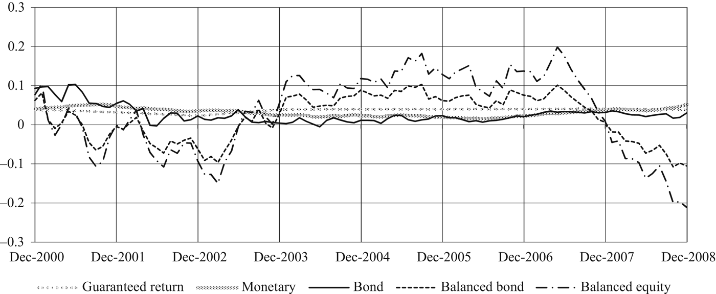
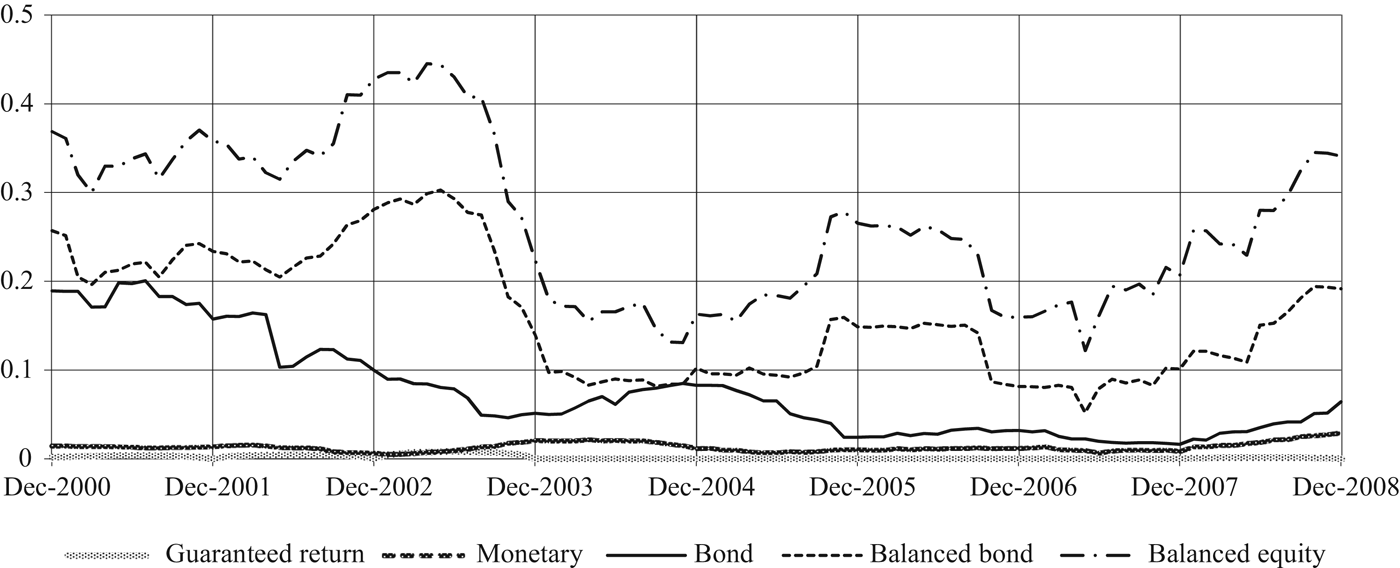
As it is apparent from Figures 1 and 2, the funds can be naturally ordered according to their returns’ volatility. The guarantee and monetary funds are by far the least volatile (with an average standard deviation respectively of 0.2 and 1.3% over the sample period), followed by the bond fund (7.5%). The two balanced funds exhibit a much higher volatility (16.1% for the balanced-bond and 26.8% for the balanced-equity).

Figure 1. Fund performance net of management fees (annualized monthly returns).

Figure 2. Standard deviation of annualized monthly fund returns.
4 Summary statistics
4.1 Participants’ characteristics
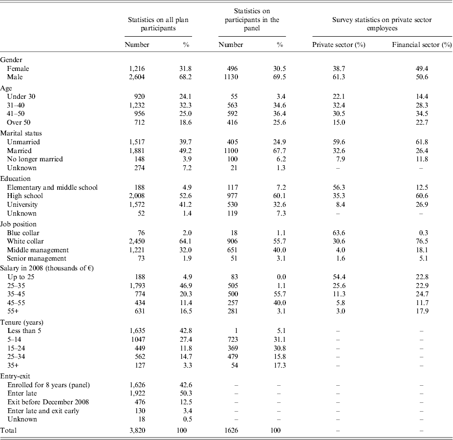
In Table 1, we present some statistics on the demographic characteristics of plan participants (information on salary, marital status and job position, as of December 2008) and compare them with those of Italian private sector workers at large, taken from the 2008 of the Bank of Italy survey on household income and wealth (SHIW).Footnote 16 Our sample differs from the Italian population in several respects.
Table 1. Statistics on plan participants (number of workers and percentages)

Workers in our sample have, on average, higher earnings than private sector workers in general and a higher level of education (94% have completed high school or college, compared with 44% of private sector employees). They are almost all clerical or managerial workers (98% of the total); mostly male (68%); relatively young (24% are <30 years old) and with relatively short job tenure (43% have <5 years of tenure). About 40% of the participants have been in the sample for all the 7 years.
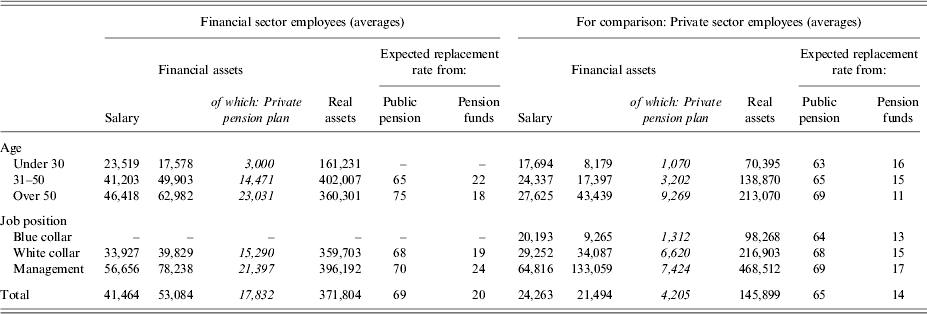
We can rely on SHIW data also for further information concerning Italian financial sector workers (Table 2). On average, they earn a net salary of about 41,000 € and have a financial wealth of about 53,000 €, of which 18,000 invested in private pension funds. Most of them are homeowners (with a real estate of about 370,000 €). Both earnings and wealth increase with age. Even if they expect most of their retirement income to come from the public pillar (replacement rate from this pillar is about 70%), the role of private pension funds is not negligible at all (with an expected replacement rate of about 20%), especially for younger workers.Footnote 17
Table 2. Income and wealth composition for workers in the Italian financial sector (Euro and percentages)

Source: SHIW 2008.
4.2 Investment choices
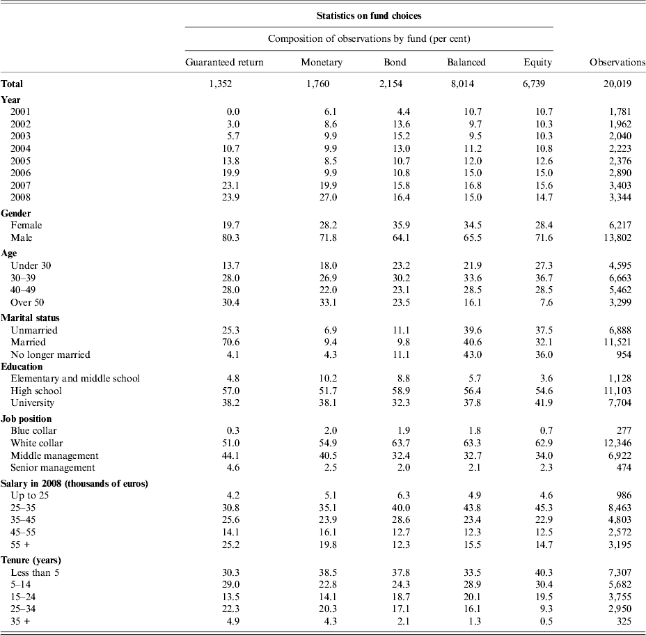
At the end of December 2008, 30% of plan participants had their wealth invested in the riskiest portfolio; 36% in the balanced one, 34% in the three remaining portfolios (Table 3).Footnote 18 Through time, there has been a shift in the relative importance of the two riskiest portfolios, which are the only ones which invest in shares: in 2002 they were chosen by 75% of participants, in 2008 this proportion drops to 65%. This is probably related to the disappointing stock market performance during the observed period.
Table 3. Statistics on choices among funds (number of observations and percentages)

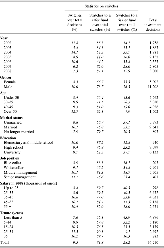
Switches only account for about 9% of all the investor-year observations: most participants confirm their previous portfolio choices most of the time (Table 4).Footnote 19 However, during our 7-years period, 25% of the 3,820 individuals observed switched at least once. The percentage rises to 48% among those that joined the plan from the start.
Table 4. Statistics on switches between funds (number of decisions and percentages)

Male and female workers do not differ much in their portfolio choices, even though females switch slightly less than males (8.5% and 9.9%, respectively).Footnote 20 With respect to education, the main difference is between the least educated group (people with only a primary school certificate) and the others. Indeed, less than 60% of the former invest in shares, compared with more than 70% in the other groups. More educated switchers are more likely to switch towards more risky funds than less educated ones. There are no clear patterns with regard to job position.
Sizable differences are apparent across age groups. In particular, while the share of workers who choose the two funds exposed to stock market risk is above 75% for those younger than 50, it drops to about 50% for those over 50. Moreover, the propensity to switch is higher for older workers, and in particular the elderly are relatively much more likely to switch towards less risky funds.
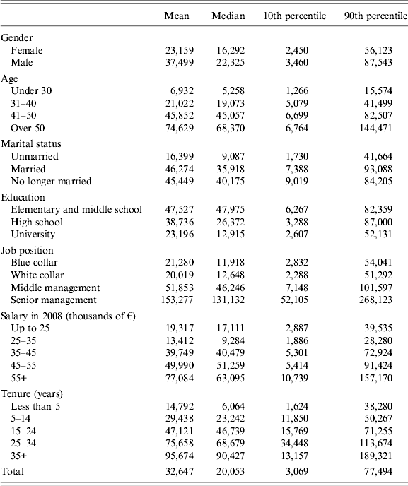
Finally, the average plan balance amounted to 32.600 € (with a median of about 20,000 €; Table 5). Not surprisingly, it increases monotonically with age, job tenure, job position and salary. Less intuitively, it decreases with education: this is due to the fact that older cohorts (which have more money in the plan) also have a lower education.
Table 5. Statistics on plan balances (€)

4.3 Performance
Looking at monthly annualized returns from 2002 to 2008, we can notice that our sample is characterized by two periods of low returns and high volatility in stock markets. The first started at end-2001 and lasted until mid-2003 and the second started in the summer of 2007, with the recent financial turmoil (Figures 1 and 2).
In particular, in 2008 the annual return of the balanced equity fund was equal to −20% while that of the balanced bond fund was −10%. Investing in one of these portfolios would have implied a severe loss in investors’ plan balances, especially harmful for older workers, given their shorter investment horizon. In this section, we try to evaluate the effects of the decision to change fund on realized returns.
First, we look at returns in the year following a switch. In the short term, changing fund has been profitable, allowing the investor to gain on average more than 1% with respect to a passive conduct.
As one-period gains or losses are more important for workers approaching retirement, which do not have the option to wait for market values to recover, we made separate computations for older investors. Workers older than 50 years who changed asset allocation at least once earned on average a return 2.9% higher than those who did not. Moreover, in 2008 older workers who switched fund avoided considerable losses which amounted on average to 25% of their plan balance, i.e., more than 22,000 €.Footnote 21
While looking at one-period-ahead returns might be a sensible approximation for older workers, this is not true for younger ones, who have a longer investment horizon. So, we also compute gains and losses for the whole sample period. We consider the individuals that were present from the start to the end of the sample and decided to change,Footnote 22 and then compare their 7 years returns at the end of 2008 to what they would have earned if they had not switched. On average, the cumulative gains from switching amount to more than 18%.
5 Multivariate analysis
5.1 The empirical model
In this section, we describe and motivate the empirical model that we bring to the data. Consider a set-up in which the indirect utility of an investor i at time t depends on the share of risky assets α it in his portfolio, on a vector of observable individual characteristics X it, and on a stochastic element ε it. More specifically, let us assume that the indirect utility function is given by U(α it; ϕit), where U is continuous in α, has the single-crossing property and ϕ i,t=βX it+ε it.Footnote 23
Suppose also that investors can choose among three types of funds (labelled 0, 1 and 2), which differ in the fraction of risky assets (α f) in their portfolios (without loss of generality, let their α f be increasing: 0 = α 0 < α 1 < α 2). It is straightforward to show that the fund chosen by the investor will be: fund 0 if βX it + ε it ⩽ K 1; fund 1 if K 1 < βX it + ε it ⩽ K 2; fund 2 if βX it + ε it > K 2, with K 1 < K 2.
If ε it is distributed according to an N(0,1) distribution, the conditional distribution of α it given X it is given in turn by:
 $$\eqalign{& P(\alpha _{it} = \alpha _0 |X_{it} ) = P(\hskip2pt\beta X_{it} + \varepsilon _{it} \lt K_1 ) = {\rm \Phi} (K_1 - \beta X_{it} ), \cr & P(\alpha _{it} = \alpha _1 |X_{it} ) = {\rm \Phi} (K_2 - \beta X_{it} ) - {\rm \Phi} (K_1 - \beta X_{it} ), \cr & P(\alpha _{it} = \alpha _2 |X_{it} ) = 1 - {\rm \Phi} (K_2 - \beta X_{it} ),} $$
where Φ is the cumulative density function of the standard normal. Equation (1) represents a multinomial ordered probit, which can be estimated using the standard maximum-likelihood techniques (Wooldridge, Reference Wooldridge2010), and this is the model that we adopt in the present paper.
5.2 Empirical results
We estimate the model described in the previous section on the pooled set of workers’ choices for the 2002–2008 period. Besides age (summarized by four age dummies), we control for gender, marital status, education and job position. In all our regressions, we also include a full set of year dummies to capture unobserved time-specific effects, among which (perceived) changes in the process driving share prices. These time dummies are also interacted with the four age dummies, to check for possible changes over time of the age effect. Our baseline specification assumes no cohort effects (however, we relax this assumption in Section 5.1).
For the sake of clarity, we merge together the guaranteed return, the money-market and the bond funds (however, we checked that results do not vary if we consider each of the five funds separately).
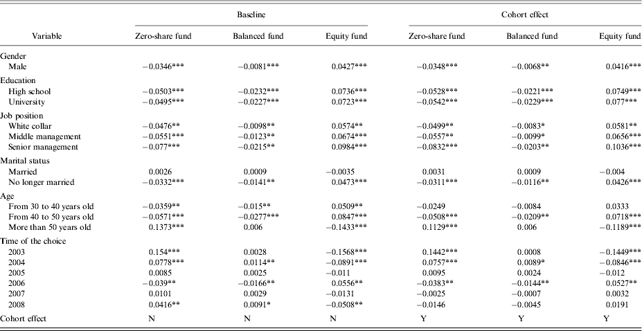
Table 6 (columns 1–3) gives our baseline estimation results. It reports the average marginal effects of a change in the independent variables on the probability to choose each fund. These figures are computed as the average effects over all individuals of our population.
Table 6. Ordered probit model: pooled regression (average marginal effects)

Note: Changes in the average probability of choosing one of the three asset allocations when the value of each dummy variable changes from zero to one for every individual.
The reference is a female, primary and middle school, blue collar worker, unmarried, in 2001. Full set of interaction terms between the age and the year dummies are included in the estimated model (omitted in the table).
Significance levels: 1% (***); 5% (**), 10% (*). Standard errors are robust to heterogeneity and autocorrelation.
Overall, the findings of the univariate analysis are confirmed. In particular, the reduction in equity-holding due to ageing is statistically significant (standard errors are clustered at the individual level). On average, the probability of being in a zero-share portfolio initially decreases and then increases with age, while the reverse is true for the probability to be in the riskiest fund.
The age–year interaction terms are statistically significant, starting from 2006.Footnote 24Table 7 shows how the probability of choosing each fund for an individual with given characteristics changes through years and age classes.
Table 7. Model-based probabilities of choosing a given fund (percentage points)

Note: Estimated probabilities implied by the model. The reference is a male, white collar, high school and married worker.
In order to better assess the economic significance of the effects we can compute the expected fraction of equities in the chosen portfolio (α it):
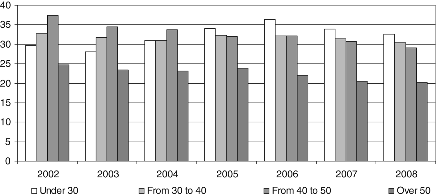
According to our estimates, the relationship between age and the holding of stock changes across time, becoming stronger at the end of the sample; moreover, while in the first years of the sample the age-stockholding profile is hump-shaped, starting from 2005, it becomes monotonically negative (Table 8 and Figure 3).Footnote 25 This may be due to the fact that workers – observing the losses suffered by their colleagues who retired during periods of declining share prices – have learnt that being exposed to stock market risk when they are near to retirement is very risky. In 2002, a married male with a white collar position and a high school degree can be expected to hold in equities a fraction of his portfolio equal to 31% if he is younger than 30, which rises to 39 if he is in his forties, then drops to 26% if he is older than 50. In 2008, these figures are 34%, 32% and 22%, respectively.

Figure 3. Model-based expected portion of equities by age and years (%).
Table 8. Expected asset allocation (percentage points)

Note: Estimated probabilities implied by the model. The reference is a male, white collar, high school and married worker. Estimated shares of stocks implied by the ordered probit model assuming that the shares are equal to 0%, 30% and 60%, respectively for the zero-share, balanced bond and balanced equity funds.
If we use age and age-squared instead of the age dummies then we can observe similar patterns. The relationship between stockholding and age turns negative at about 40, while in Agnew et al. (Reference Agnew, Balduzzi and Sunden2003) the peak is reached at about 30.
Like the final decrease, the initial increase in the fraction of stocks is consistent with optimal portfolio theory, as the young are relatively more exposed to labour market risks (Campbell and Viceira, Reference Campbell and Viceira2002).
Concerning controls, being male, having a better job position and a higher education decreases the probability of choosing a zero-share portfolio and increases the probability of choosing the riskiest portfolio in a statistically significant way.
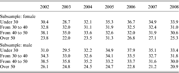
To investigate further the role of gender, we estimate separately the age-portfolio profiles for men and women.Footnote 26 It appears that, while in most years of the sample males start their career with a slightly riskier portfolio with respect to females, they are also relatively quicker (at least in the second half of the sample period) in moving towards safer assets as they age (Table 9a). This result is in line with the results by Barber and Odean (Reference Barber and Odean2001a), who show that men tend to trade more than women.
Table 9a. Expected asset allocation (percentage points)

Note: Probabilities implied by the model estimated on different subgroups. The reference is a white collar, high school and married worker. Estimated shares of stocks implied by the ordered probit model assuming that the shares are equal to 0%, 30% and 60% respectively for the zero-share, balanced bond and balanced equity funds.
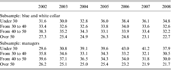
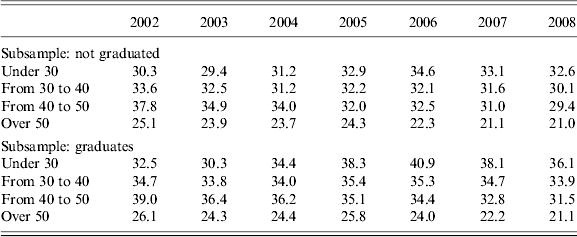
Interestingly, a similar pattern emerges if we estimate the model separately for managers and non-managerial workers (Table 9b), and if we distinguish between workers with and without a university degree (Table 9c). Both managers and graduates start their careers with relatively more risky assets in their portfolio, but both categories are relatively faster in moving towards less risky assets. This behaviour might be related to the fact that they have easier access to financial information and/or a higher level of financial literacy (documented among others by Van Rooij et al., Reference van Rooij, Lusardi and Alessie2011).
Table 9b. Expected asset allocation (percentage points)

Note: Probabilities implied by the model estimated on different subgroups. The reference is a male, high school and married worker. Estimated shares of stocks implied by the ordered probit model assuming that the shares are equal to 0%, 30% and 60%, respectively for the zero-share, balanced bond and balanced equity funds.
Table 9c. Expected asset allocation (percentage points)

Note: Probabilities implied by the model estimated on different subgroups. The reference is a male, white collar and married worker. Estimated shares of stocks implied by the ordered probit model assuming that the shares are equal to 0%, 30% and 60%, respectively for the zero-share, balanced bond and balanced equity funds.
6 Extensions and robustness checks
6.1 Modelling cohort effects
As it is well known, due to collinearity it is impossible to separately identify cohort, time and age effects without imposing some additional identification restriction to the data-generating process. In the estimates of Section 5, we followed Agnew et al. (Reference Agnew, Balduzzi and Sunden2003), therefore we controlled for time and age effects while assuming the absence of cohort effects. In this section, however, we relax this assumption and enrich our baseline model by adding cohort effects. To do this, we use the identification strategy pioneered by Malmendier and Nagel (Reference Malmendier and Nagel2011). These authors argue that portfolio choices of people belonging to the same cohort are similar because they went through similar economic and financial experiences and in particular, they experienced the same stock market returns during their lifetime. Therefore, we enrich our specification to include the Malmendier and Nagel (Reference Malmendier and Nagel2011) proxy for the cohort effect, namely the average yearly returns of the Italian stock market over the lifetime of each individual. Remarkably, this leaves unaffected the magnitude and significance of the age effect (Table 6, columns 4 to 6).
6.2 Fixed-effects estimation
As we remarked in the introduction, one limit of administrative records is that they do not contain much information about participants’ characteristics. The possibility of a bias in our estimates due to omitted variables is therefore a source of concern. In the present section, we address this problem by estimating a fixed-effect model, which allows us to control for the effect of all the unobserved time-invariant characteristics of the participants.
We make two departures with respect to our baseline model: first, we use a logit instead of a probit distribution function; second, we model age as a quadratic function instead of a set of age-dummies. The first departure is needed because there is no way, to our knowledge, to account for unobserved individual heterogeneity within a multinomial probit model whereas in the multinomial logit case we can resort to some recent papers and in particular to Baetschmann et al. (Reference Baetschmann, Staub and Winkelmann2011). The second departure is needed because the Baetschmann et al. (Reference Baetschmann, Staub and Winkelmann2011) estimation technique does not exploit the information provided by all those individuals that never switch between funds. This entails a sharp decrease in the degrees of freedom that induced us to resort to a more parsimonious specification of the age effect.
In our setting, where the dependent variable can take three values (e.g., 0, 1, 2), the Baetschmann et al. (Reference Baetschmann, Staub and Winkelmann2011) procedure requires the creation of two dichotomous variables (d i,t 1, d i,t 2). The first is equal to one if and only if the chosen fund is the one with the highest share of risky assets; the second is equal to one if the chosen fund is not the safe one, i.e. (using the notation introduced in Section 5.1):
 $$\eqalign{& d_{i,t}^1 = I(\mu _i + \beta X_{it} + \varepsilon _{it} \gt K_1 ), \cr & d_{i,t}^2 = I(\mu _i + \beta X_{it} + \varepsilon _{it} \gt K_2 ),} $$
where I(·) is the indicator function and μ i is the individual fixed effect. The second step of the procedure requires the estimation of two binary logit-fixed effects models for d i1,t and d i2,t as in Chamberlain (Reference Chamberlain1980). Indeed, Chamberlain (Reference Chamberlain1980) shows that maximum-likelihood estimation of a binary logit-fixed effects model conditional on the sum of all the outcomes over time gives consistent estimates. In the final step of the procedure, a weighted sum of the two estimates obtained in the second step is computed.Footnote 27
The second column in Table 10 shows that the estimated age effects obtained using the Baetschmann et al. (Reference Baetschmann, Staub and Winkelmann2011) procedure confirms our baseline results: the coefficients on age and age-squared are highly significant and the stock-holding/age profile has a hump-shaped pattern, with a peak at 40.
Table 10. Estimations of the age effect: robustness exercises (parameter estimates)
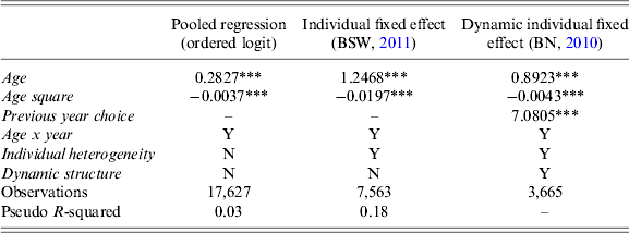
Note: Baetschmann et al. (BSW, Reference Baetschmann, Staub and Winkelmann2011) map the categorical response into a set of binomial variables, so that a fixed-effect binomial logit can be estimated. Bartolucci and Nigro (BN, Reference Bartolucci and Nigro2010) propose a statistical model that allow dynamic fixed-effect, we apply it on the specification proposed by Baetschmann et al. (Reference Baetschmann, Staub and Winkelmann2011).
6.3 Fixed-effects estimation controlling for dynamics
The choice of the fund in period t might depend on previous choices. This would be the case if investors tend to stick to their status quo (inertia in financial decisions has been documented in a number of studies, among which Bilias et al., Reference Bilias, Georgarakos and Haliassos2010). Past choices would matter also if investors are relatively more responsive to the performance of their own fund. The specification used in the previous section cannot account for such dynamic effects, as lagged values of the dependent variable are not among the regressors. To allow for this possibility we extend the dynamic fixed-effect binary logit model recently developed by Bartolucci and Nigro (Reference Bartolucci and Nigro2010) to our trichotomous setting.Footnote 28
Bartolucci and Nigro (Reference Bartolucci and Nigro2010) proposed the following binary model:
where d i,t is a dichotomous variable, μ i is the individual fixed effect, and e*(μ i,Xi) is a variable which can be interpreted as a measure of the effect of the present choice d i,t on future expected utility. We apply the Baetschmann et al. (Reference Baetschmann, Staub and Winkelmann2011) procedure described in the previous section to the model in equation (3) instead of applying it to a Chambelain-style static fixed effect binary logit as Baetschmann et al. (Reference Baetschmann, Staub and Winkelmann2011) do. Namely, we estimate equation (3) for the two dicothomous variables described in equation (2), and build an estimate of the impact of X it on the original trichotomous variable using a weighted average of the estimates concerning the two dicothomous variables d i1,t,di 2,t.
The results of this procedure confirm the relation between asset allocation and age found in our baseline exercise (Table 10, column 3). Moreover, the dynamic factor turns out to be significant, suggesting that portfolio choices are indeed persistent.Footnote 29
6.4 Conditional switching probabilities
In order to investigate the role of inertial behaviour in workers’ choices in this section, we can also focus specifically on shifts from one fund to another.
To this aim, we run our baseline regression conditional on the fund chosen in the previous year. Besides being interesting per se, this exercise can be also seen a simple way to control for both dynamic effects and unobserved heterogeneity, alternative to the one discussed in Section 6.2. In particular, it has the advantage that we can use our baseline specification, and that it does not ignore the information concerning the participants that never switch fund.
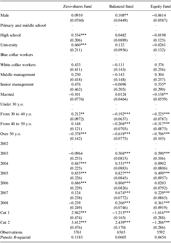
We proceed in two steps. First, we run our baseline regression on different subsamples, grouping people according to the fund that they chose in period t−1 (Table 11). As before, dependent variables include dummies for gender, education, job position, marital status, years and age.
Table 11. Ordered probit model: separate regressions (parameters estimates)

Note: The table shows parameter estimates of ordered probit models run separately for participants starting from a zero-share, balanced bond and balanced equity funds.
The reference is a female, primary and middle school, blue collar, unmarried, under 30 y.o., 2002. Significance levels: 1% (***); 5% (**), 10% (*).
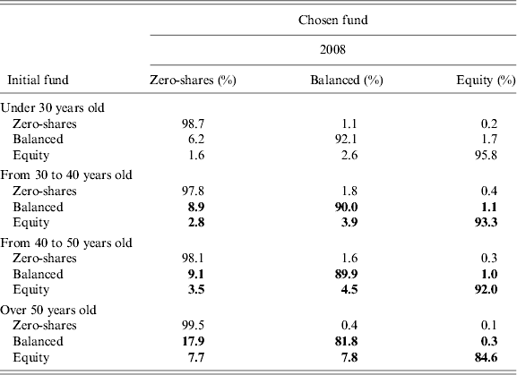
Second, we use the estimated parameters to compute the conditional probability of switching from one fund to another. The probabilities are summarized in conditional transition matrices (Tables 12 and 13).Footnote 30 The elements on the main diagonal of each matrix give, for a particular participant (e.g., a male, middle manager, higher educated, unmarried participant choosing his retirement account asset allocation in 2008), the probability of remaining in the old fund; on the contrary, the elements off the main diagonal give the probability of switching from the fund on the row to the one on the column. We compute different matrices for alternative settings of the X variables in order to assess the impact of each covariates. All in all, this approach is analogous to that of Bertaut (Reference Bertaut1998).Footnote 31
Table 12. Model-based conditional transition matrix by age (percentages)

Note: The reference individual is a 30-to-40 years old male worker, white collar, with a high school degree and married. The percentages show model-based probabilities to switch form the initial fund (rows) to the chosen fund (columns). Probabilities in bold are statistically different from those of the reference matrix at the 5% significance level.
Table 13. Model-based conditional transition matrix by year (percentages)

Note: The reference individual is a 30-to-40 years old male worker, white collar, with a high school degree and married. The percentages show model-based probabilities to switch form the initial fund (rows) to the chosen fund (columns). Probabilities in bold are statistically different from those of the reference matrix at the 5% significance level.
The age effect highlighted in the previous sections is again quite strong (Table 11). The probability of remaining in the riskiest fund is 96% for a less than −30 y.o. worker, falling to 85% for a 50+ y.o. worker. Moreover, the probability of switching towards less risky funds starting from the balanced one is much lower for the young than for the old participant (6% versus 18%).
The likelihood of switching towards less risky portfolios is higher at the beginning and at the end of the sample, when the returns from the stock market were particularly disappointing. In 2005 (a year of relatively bullish markets), the probability of not changing fund was 95% for those starting in the riskiest fund and 93% for those starting in the balanced fund. These probabilities were, respectively, 93% and 90% in 2008, and 87% and 86% in 2002 (Table 13). Most importantly, the probability of switching towards riskier funds for those in the zero-equities portfolios was much lower during the end-of-period and the beginning-of-period stock market crashes: indeed, for those starting from the no-shares funds, the probability was 18% in 2005, compared with 4% and 2%, respectively in 2002 and 2008. The effects of sex and job position on the probability of switching are not statistically significant (results not shown), as in the sample these are basically time-invariant characteristics. This result is different from what we found in the previous section, in which we studied the unconditional probability of choosing a particular fund.
So far, we focused on annual conditional probabilities. In the context of retirement saving we might want to evaluate probabilities over a longer horizon. For example, we might be interested in the model-based probability that a 35 years old plan participant who invests in the equity fund will end up 20 years later in the zero-share fund. We can compute this probability using the transition matrices for 2008 in Table 12. For example, if we consider a married man, white-collar, with a high-school degree, and assume that his job-position does not change over time, there is 86% chance that by the end of the 20 years period he will be found in the zero-share fund. Alternatively, if we use the transition matrix for 2005, a year of positive returns, such probability goes down to 42%. We could be more accurate and allow for the fact that the years of negative and positive returns evolve stochastically over time; however, our simple exercise can be seen as giving reasonable lower and upper bounds.
7 Conclusions and suggestions for further research
We studied investors’ portfolio choices in a very simple and clear-cut real-world setup. Some results prove quite robust across all the empirical exercises we performed. First, there is a tendency to choose safer funds as people age. This effect is still there after controlling for several demographic factors, for time effects, for the fund chosen in the previous period, for individual fixed effects (in a static as well as in a dynamic specification) and cohort effects (modelled as in Malmendier and Nagel, Reference Malmendier and Nagel2011).
However, the effect is non-linear, being much stronger in the very last years of the career. Moreover, not all elderly people in our sample reduced their exposure to risk. Looking at the ones present in the sample from the start, it turns out that more than 30% of the elderly workers, which were exposed to stock market risk in 2001 were still exposed to it in 2008. More generally, the significance of the persistence parameter in our dynamic estimates signals a possible status quo bias.
An elderly worker taking risk on the stock market could pay a high price if stocks fall. To the extent that this inertia is related to behavioural factors, there might be room for welfare-improving policy interventions. For example, the diffusion of life cycle funds could be promoted. This kind of investment vehicles automatically brings all the participants towards less risky allocations as they age (Viceira, Reference Viceira2007). In the Chilean system, for example, a lifecycle fund is the default option for all the workers. Moreover, the riskiest funds are closed to individuals older than a certain age.
We also document that the effect of age is more pronounced in the last years of the sample. This might be due to the fact that investors learn from the experience of their colleagues. Indeed, in our sample there have been periods of disappointing stock market performance. Having seen that people who retired during these bear market periods have been severely hit might have pushed investors towards a more active behaviour. A better understanding of this form of learning appears to be an interesting issue for further research.
We find that job position has an impact on portfolio choice (but not on the probability of switching): people with a higher position tend to take more risks. This tallies with previous empirical analyses and can be consistent with optimal portfolio allocation (Brunnermeier and Nagel, Reference Brunnermeier and Nagel2008; Chiappori and Paiella, Reference Chiappori and Paiella2008; Cappelletti, Reference Cappelletti2009). Finally, we find that education also increases both the share of stocks in the portfolio and the likelihood of switching for those in the zero-shares funds.
Before concluding, we would like to remark that the fact that the behaviour of most workers is by and large consistent with optimal portfolio theory does not rule out other possible interpretations of our results. For example, if investors pay more attention to retirement savings when they are older (because retirement is more salient or because the plan balance is bigger), and if attentive individuals tend to move towards saver portfolios (maybe because the sample period is overall a period of disappointing stock market performance), this could explain why workers leave risky investments as they age. An increased use of advisory services by older workers would be evidence in favour of this interpretation.Footnote 32


