1 Introduction and summary

What has been the impact on public pension funds’ Unfunded Accrued Liabilities (UAL) of the gap between assumed and actual investment returns, over extended periods? How has this impact compared with that of other factors that raise the UAL? An influentialFootnote ¹ approach to this question (Munnell et al., Reference Munnell, Aubry and Cafarelli2015) takes the components of the actuarial gain/loss statement from a plan's annual valuation reports, and simply adds them up over time. In this paper, I critique the methodological basis for this procedure and propose a sound replacement. I find that the method in question significantly low-balls the impact of the gap in investment returns in many cases. The policy implication is to under-emphasize the need to cut the assumed return on investment.

The procedure's problem arises in the last step. Even if the annual gain/loss components of the rise in UAL are accurate, adding them up over a period of years to arrive at a cumulative breakdown of the multi-year rise in UAL is problematic. The reason is that this procedure, which I shall call the simple summation (SS) method, does not realistically model the subsequent amortization payments triggered by any rise in UAL. Instead of using the actual amortization policy, the method implicitly assumes amortization rises to cover the interest on the UAL.

For example, if the UAL rises by $100, due to the gap in investment returns, the SS method assumes the following year's amortization payments will rise by the interest on that $100, e.g., $8.00 under a typical assumed return of 8%. However, under the actual amortization formula commonly used (‘level percent of payroll’), those payments will often rise by a lesser amount. With parameters of 4% payroll growth and 30-year amortization, the payment would be $5.90, or $2.10 short of covering the interest. Consequently, the initial $100 impact on the UAL will rise over a multi-year period with accrued unpaid interest. By analogy, the financial impact of a $100 credit card debt will grow over time if the user's policy is to not pay the full interest. In the public pension context, this will be the case when the amortization schedule is back-loaded, under policy choices that combine long amortization periods, high assumed payroll growth (which tilts the schedule up), and high assumed investment return (since that is the interest rate that accrues on the UAL).

By contrast, the SS method holds the initial $100 impact constant by assuming payments rise $8.00 to cover the additional interest, instead of following the actual amortization formula. The SS method attributes the subsequent rise in UAL from accrued unpaid interest ($2.10 in the first year) to contribution shortfalls instead of the gap in investment returns that triggered it. As a result, the SS method will often underestimate the multi-year impact of the gap in returns (or anything else that raises the UAL). As I will show, with the example of the Connecticut State Teachers’ Retirement System, this underestimate can be substantial.

It is important to get the impact of the gap between assumed and actual returns right, not only for academic reasons, but also for practical policy purposes. In the aftermath of the 2007–2009 market crash, many funds reduced their assumed returns, but not by much (0.27%, on average, Biggs, Reference Biggs2015). Several years later, the cuts have in many cases proven insufficient to prevent a further rise in UALs. Thus, pension policy-makers – and the general public – need to understand the full impact of high assumed returns to better motivate rate-cutting policy going forward. By underestimating the past impact, the SS method can lead policy-makers to place less emphasis on reducing the assumed return than is warranted. At the same time, the important intertemporal interaction between the amortization policy and the UAL-drivers reinforces the need to keep the amortization period short and the assumed payroll growth low.

The underlying problem with the SS method is that it has emerged without careful attention to the counterfactual scenarios it purports to address, such as, ‘What if investment returns had met assumptions, while other UAL-drivers remained unchanged?’Footnote ² Under the SS method, the key ‘other’ UAL-driver is the contribution shortfall between interest on the UAL and amortization.Footnote ³ Thus, in the counterfactual for the gap in investment returns the contribution shortfall is held fixed (at its actual value). This is where the implicit assumption regarding amortization creeps in. If the contribution shortfall is held fixed, then amortization varies dollar-for-dollar with the interest on the counterfactual UAL. To restate the example given above more precisely, if the UAL had been $100 lower in this counterfactual (as assumed returns were met), the subsequent amortization would have been reduced by the full $8.00 interest on that $100, thereby attenuating the subsequent counterfactual drop in UAL. Thus, the difference between the actual UAL and the counterfactual UAL at the end of the period – the multi-year impact of the gap in investment returns – is underestimated. This is the crux of the problem.

The SS method also yields untenable results on other UAL-drivers. Most strikingly, under this method the cumulative UAL impact of pension obligation bonds (POBs) is no different from the initial impact of receiving the proceeds. If a state issues POBs to ‘pay down,’ say, $2 billion in a fund's UAL (as did Connecticut for its teachers’ fund in 2008) the plan's annual gain/loss statement will record a $2 billion reduction in the UAL that year due to the POB. The problem is that in the SS multi-year analysis, the cumulative impact remains at $2 billion every year thereafter. There is no impact attributed to the POB of the return on the proceeds invested in the fund (let alone the outstanding POB debt incurred by the state). Indeed, even if the invested proceeds quickly lose substantial value – as happened in Connecticut – this will have no effect on the cumulative impact under the SS method. This is clearly misleading.

The structure of the paper is as follows. First, I review the analytics behind the SS method. Next, I dissect the key issue of how the method's counterfactual model of amortization diverges from actual amortization formulas, and draw its implications. I then illustrate my proposed method of using actual amortization formulas. To complement our understanding of the impact of UAL-drivers under the different amortization assumptions, I show that the difference is mirrored in the impact on cumulative contributions. The total impact – paid and not-yet-paid (amortization and UAL, respectively) – is essentially invariant. Finally, I show how the SS method provides an unsatisfactory treatment of POBs, due to its implicit amortization assumption, and that a correct treatment can qualitatively reverse the measured impact of the POBs on the UAL, as in the Connecticut case.

It is important to note that under my method, the sum of the UAL impact of individual drivers will not sum to the actual rise in the UAL, unlike the SS method. That is because of the intertemporal interactions that are recognized in my method, but effectively assumed away under the SS method. The important interaction here is between the gap in investment returns and the actual amortization formula. If the gap in returns raises UAL, but amortization does not cover the ensuing additional interest, then the UAL rises further – a result attributable to the gap in returns. If we separately consider the impact of payments that fail to cover interest, the accrued unpaid interest would appear in both impacts. Hence, the non-additivity. The SS method is additive, but only because, in calculating the impact of the gap in returns, it replaces the actual amortization formula with an artificial formula that covers the ensuing additional interest. The result is more aesthetic, but less policy-relevant. If the user's interest is the impact of the gap in investment returns, we should use the actual amortization formula to answer that question. Additivity is also not necessary to compare policies. Even if we cannot parcel out the rise in UAL as X percent from the gap in investment returns and Y percent from contribution shortfalls, we can still compare each factor's impact. The key policy implication of my method is that it will often show a much larger impact of the gap in investment returns, relative to contribution shortfalls, than does the SS method.

Throughout the paper, I supplement the analytical results with illustrations adapted from the Connecticut State Teachers’ Retirement System (CSTRS), FY00-FY14.The CSTRS case is of interest in its own right for several reasons. The system's pension funding difficulties rival those of such well-known cases as California, New Jersey, Illinois and Pennsylvania. Unlike other systems, it did not reduce its assumed rate of return from 8.5% over this period. Finally, it has made use of POBs to ‘pay down’ its UAL. Thus, it is an interesting case to illustrate the effect of using a more sound method of assessing the impact of the gap between assumed and actual investment returns, as well as the impact of POBs.

2 The sources of the rise in UAL: the SS method

The starting point is the decomposition of the annual rise in UAL presented in a plan's valuation report. The sources of the rise can be categorized into: (i) the gap between assumed and actual investment returns; (ii) contribution shortfalls, between interest on the UAL and amortization payments; and (iii) adverse liability developments (changes in and deviations from actuarial assumptions, as well as benefit changes).Footnote ⁴

Let us consider this decomposition formally, with some slightly simplified math:Footnote ⁵

(1) $${\rm UAL}_t \equiv L_t - A_t $$

(2) $$L_t = (L_t - L_{t \vert t - 1}^e ) + L_{t \vert t - 1}^e = (L_t - L_{t \vert t - 1}^e ) + (1 + r{^\ast})L_{t - 1} + {\rm NC}_t - B_t $$

(3) $$A_t = (1 + r_t )A_{t - 1} + {\rm AMT}_t + {\rm NC}_t - B_t, $$

where A _t  = assetsFootnote ⁶ ; L _t  = accrued liabilities; $L_{t \vert t - 1}^e $  = expected accrued liabilities in period t, as of t − 1, under actuarial assumptions; NC _t  = normal cost; B _t  = benefit payments; AMT _t  = employer contributions in excess of NC, credited toward amortization; and r*, r _t  = assumed and actual return on investment.Footnote ⁷

Substituting and simplifying, we have the standard actuarial gain/loss result, decomposing the change in the UAL from t − 1 to t:

(4) $$\Delta _{t - 1,t} {\rm UAL} = (r{^\ast} - {\rm} r_t )A_{t - 1} + (r{^\ast}{\rm UAL}_{t - 1} - {\rm AMT}_t ) + (L_t - L_{t \vert t - 1}^e ).$$

The first term on the right-hand side is the loss from the gap in investment returns; the second term is the loss from any failure of amortization to cover interest on the UAL; and the third term is the loss from liabilities exceeding expectations (for the reasons given above).

For the 1-year change in UAL, this is an attractive formulation: it unambiguously allocates ΔUAL among the gap in investment returns, contribution shortfalls, and liability losses in a way that adds up to the actual change in the UAL. There are no interactions to disrupt additivity. As shown below, interactions will arise from the lagged values of UAL and A in the multi-year ΔUAL, but for the 1-year change, these are pre-determined. Thus, each term in (4) answers a well-defined counterfactual question about factors that are independent of one another: ‘How would the UAL in period t (and its rise from period t − 1) differ from the actual if, in period t, investment assumptions had been met (or amortization had covered interest, or liability assumptions had been met)?’

How, then, to allocate the rise in UAL over multiple periods, from period 0 to T? The approach put forth by Munnell et al. (Reference Munnell, Aubry and Cafarelli2015) at the Center for Retirement Research at Boston College is to simply add up each component of (4), year-by-year, to allocate the total change in the UAL among its various sources:

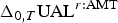
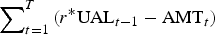
(5) $$\eqalign{\Delta _{0,T} {\rm UAL} &= \sum\limits_{t = 1}^T {(r{^\ast} - r_t )A_{t - 1}} + \sum\limits_{t = 1}^T {(r{^\ast}{\rm UAL}_{t - 1} - {\rm AMT}_t ) }+ \sum\limits_{t = 1}^T {(L_t - L_{t \vert t - 1}^e )} \cr &= \Delta _{0,T} {\rm UAL}^{r:{\rm \Sigma}} + \Delta _{0,T} {\rm UAL}^{C:{\rm \Sigma}} + \Delta _{0,T} {\rm UAL}^{L:{\rm \Sigma}}.} $$

The first line is correct: the rise in UAL from period 0 to T equals the T-period sum of each term in (4). The issue is the interpretation, term by term, in the second line. I label each term as the contribution to the rise in UAL from the three UAL-drivers, as attributed by the SS method: Δ_0,T UAL ^r:Σ, etc., where Σ denotes the simple summation from the annual gain/loss statements. (I use C in the second term to denote contribution shortfalls, C _t  ≡ r*UAL _t−1 − AMT _t .) This interpretation purports to answer the T-period version of the questions given above: ‘How would the UAL in period T (and its rise from period 0) differ from the actual if, in periods 1,…,T, investment assumptions (for example) had been met and the series of other drivers held at their actual values?’ Before exploring this question in depth, I illustrate the method's results with data from the CSTRS.

I use an adaptation of the CSTRS time series for FY00–FY14.Footnote ⁸ The main differences between this adaptation and the actual series are the use of market asset values rather than smoothed values and the exclusion here of the $2 billion FY08 POB, to be considered separately below.Footnote ⁹ The net result of these adaptations is a rise in the UAL of $10.4 billion from FY00 to FY14, rather close to the actual rise of $10.6 billion (excluding the $2 billion POB proceeds).

Figure 1 depicts the decomposition of the $10.4 billion rise under the SS method. I find that this method attributes $5.0 billion to the gap between the assumed investment return of 8.5% and actual investment returns (red line), Δ_0,T UAL ^r:Σ. Contribution shortfalls (purple line) account for another $3.3 billion, Δ_0,T UAL ^C:Σ.Footnote ¹⁰ Thus, under this method, the impact of the gap in investment returns exceeds that of the contribution shortfalls by 50%.Footnote ¹¹

Figure 1. ΔUAL, Simple summation method: C _t exogenous. CSTRS, FY00–FY14 adapted from CSTRS: market asset values, without midyear return on cash flows and accruals.

I have broken out liability losses into those due to actuarial assumptions and benefit enhancements, of which there was only one, in FY08.Footnote ¹² In Fig. 1, note that the cumulative impact of the FY08 benefit hike, $\Delta _{0,T} {\rm UAL}^{L({\rm benefits}):{\rm \Sigma}} $ , is unchanged beyond FY08: the brown line is flat.Footnote ¹³ Indeed, under the SS method, the 1-year impact of any contributor to the rise in UAL, as specified in (4), is also the cumulative impact thereafter, in (5). Specifically, there is no further impact from the interest on the initial change in UAL. As explained below, that is because the method implicitly assumes amortization payments will be adjusted to cover the interest.

3 How does amortization behave in the implicit counterfactual?

Where does the implicit assumption about amortization come from? It is embedded in the counterfactual question underlying the SS method's decomposition in (5): ‘How would the UAL in period T differ from the actual if investment assumptions (for example) had been met and the series of other drivers held at their actual values?’ The counterfactual scenario has not been explicitly analyzed before,Footnote ¹⁴ but can be readily uncovered by comparing the actual Δ_0,T UAL in (5) with the counterfactual Δ_0,T UAL if investment assumptions had been met, r _t  = r*:

(5 CF^r ) $$\Delta _{0,T} {\rm UAL} = \sum\limits_{t = 1}^{^T} {(\underline {r{^\ast} - r{^\ast}} )A_{t - 1}} + \sum\limits_{t = 1}^T {(r{^\ast}{\rm UAL}_{t - 1} - {\rm AMT}_t )} + \sum\limits_{t = 1}^T {(L_t - L_{t \vert t - 1}^e )}.$$

Subtracting (5 CF^r ) from (5), we get $\sum\nolimits_{t = 1}^T {(r^{\ast} - r_t )A_{t - 1}} $ , since the first term of (5 CF^r ) is zero. This is Δ_0,T UAL ^r:Σ, the SS method's attribution of the rise in UAL to the gap in investment returns, as given on the second line of (5). This is the procedure underlying the method's decomposition.

This procedure implicitly assumes the other two terms in (5) and (5 CF^r ) are equal. Specifically, the series of contribution shortfalls and liability losses are held exogenous at their actual values while the gap in investment returns is assumed to vanish. This is certainly a defensible assumption for liability losses – there is no obvious link between them and the counterfactual investment returns.

The sticking point here is the implicit assumption that the counterfactual series of contribution shortfalls is the same as the actual, i.e., C _t is taken as exogenous under the SS method. Since the contribution shortfall is the gap between amortization payments and interest on the UAL, this means the counterfactual amortization must vary with the counterfactual interest to maintain C _t . That is, it is implicitly assumed that in the counterfactual with r _t  = r*,

(6) $${\rm AMT}_t = r{^\ast}{\rm UAL}_{t - 1} - C_t, $$

where C _t is held constant at the actual level. Thus, in this counterfactual, where UAL _t−1 is reduced from the actual, it is implicitly assumed that subsequent amortization would also be reduced, dollar-for-dollar with the interest on the UAL. (This assumption is also embedded in the counterfactual on liabilities.) The problem is this is not how amortization formulas work: amortization would commonly drop by less than the interest (although theoretically, it could drop by more, depending on the formula's parameters).

Specifically, the formula commonly employed is ‘level percent’ of payroll. With assumed payroll growth rate g, the basic form is:Footnote ¹⁵

(7) $${\rm AMT}_t = {\rm UAL}_{t - 1} (r{^\ast} - g)/\{ 1 - [(1 + g)/(1 + r{^\ast})]^{\rm N}\}, $$

where N is the remaining amortization period (closed or open). We can then write

(8) $${\rm AMT}_t = \alpha _t (r{^\ast}{\rm UAL}_{t - 1} ),$$

where $\alpha _t = [(r^{\ast} - g)/r^{\ast}]/\{ 1 - [(1 + g)/(1 + r^{\ast})]^N \}. $ The key points here, in comparison with (6), are: (i) amortization is proportional to the interest on the UAL, so there is no constant term as in (6) (−C _t ); and (ii) the coefficient on the interest, α _t , can be less (or greater) than one, unlike (6). Indeed, if C _t  > 0 (interest exceeds amortization, as is true on average, according to Munnell et al., Reference Munnell, Aubry and Cafarelli2015), then α _t must be less than one. In other words, if there is a contribution shortfall under a proportional amortization formula, that directly implies amortization varies less than dollar-for-dollar with interest on the UAL, contrary to the implicit assumption of the SS method. This is the crux of the problem with the method – the main reason SS underestimates the impact of the gap in investment returns, as explained below.

The difference between (6) and (8) is illustrated in Fig. 2, which depicts counterfactual values of AMT _t on the vertical axis and counterfactual values of r*UAL _t−1 on the horizontal. Equation (6) is parallel to the 45° line (AMT _t  = r*UAL _t−1), shifted down by a constant equal to the actual contribution shortfall, C _t . Equation (8) is a clockwise rotation of (6), through their common point, the actual value of (r*UAL _t−1, AMT _t ). This shows visually that if there is a contribution shortfall (C _t > 0) under a proportional amortization formula, the marginal response of amortization to a change in the interest on UAL (the slope of (8)) must be less than one (the slope of (6)), as assumed under the SS method.

Figure 2. Counterfactual AMT _t as function of counterfactual r*UAL _{t −1} under exogenous C _t , and exogenous α _t .

What policy variables, under control of the pension fund, generate this condition? That is, what combinations of r*, g, and N result in α _t  < 1 in (8)? If the payment scheduled is back-loaded, payments may not cover interest. This will be true for combinations of long amortization periods, high assumed payroll growth (since high g lowers the initial payments)Footnote ¹⁶ and high assumed returns (since the interest is r*). Formally, for any given value of N, we can derive a level curve for α _t in (r*, g), above which α _t  < 1, as depicted in Fig. 3. For example, at the common values of N = 30 and r* = 0.075, any g > 0.013 will generate contribution shortfalls. Calculating (8) for those plans in the BC Public Plans database that are coded as ‘level percent’ and which report g, I find almost all of them are characterized by α _t  < 1, with r* ≥ 0.075 and g ≥ 0.03.Footnote ¹⁷ My proposed alternative to the SS method replaces the implicit assumption that C _t is exogenous (so α _t  = 1) with the assumption that α _t is exogenous at the actual observed value.

Figure 3. Level curves of g and r* for α = 1 (above the curves, α < 1).

4 What are the implications of taking C _t as exogenous?

Before spelling out my alternative, I can sketch the implications of the SS method's treatment of C _t as exogenous. The main implication is that the SS method will underestimate the impact of the gap in investment returns if α _t  < 1, (and, conversely, if α _t  > 1). The reason is that under the SS method, if the gap in returns generates an increment to the UAL and to the interest on the UAL the following year, amortization is implicitly assumed to cover the incremental interest, adding nothing to the contribution shortfall. But if the actual amortization process only partially covers additional interest (α _t  < 1), there will be an additional contribution shortfall, induced by the gap in investment returns.

This can be understood in terms of equation (5). Under the SS method, the gap in investment returns raises the UAL directly through the second term of (5), $\sum\nolimits_{t = 1}^T {(r^{\ast} - r_t )A_{t - 1}} $ , with no indirect impact through the third term, $\sum\nolimits_{t = 1}^T {(r^{\ast}{\rm UAL}_{t - 1} - {\rm AMT}_t )} $ , since it remains unchanged by implicit assumption that C _t is exogenous. But if amortization is actually governed by (8) with α _t  < 1, there will be an additional contribution shortfall induced by the gap in investment returns, reflected in the third term of (5). In short, there is a significant intertemporal interaction between the gap in returns and an amortization regime that generates contribution shortfalls.

The SS method's treatment of C _t as exogenous also explains the puzzling time pattern of other drivers’ impact. Consider CSTRS’ FY08 enhancement to the cost-of-living adjustments (COLA) that raised the UAL by $1.15 billion. As Fig. 1 shows (brown line), under the SS method, the cumulative impact remains unchanged thereafter. There is no further measured impact from the accumulation of interest on the additional UAL because of the implicit assumption that additional amortization covers that interest. If, instead, the amortization regime does not fully cover additional interest (α _t  < 1), there would be additional contribution shortfalls, induced by the benefit enhancement. The SS method assumes away the interaction between the benefit enhancement (or any other liability loss) and an amortization regime that underfunds the interest on the UAL.

5 Endogenizing asset values, for consistent counterfactuals

There is another problem with the SS method that needs to be fixed, before presenting the full alternative. That is the exogenous treatment of asset values in the counterfactuals for liability losses and contribution shortfalls. In constructing the counterfactuals underlying Δ_0,T UAL ^L:Σ and Δ_0,T UAL ^C:Σ in (5), the term $\sum\nolimits_{t = 1}^{^T} {(r^{\ast} - r_t )A_{t - 1}} $ is taken to be the same in the counterfactual as in the actual. That means the series of asset values A _t is taken as exogenous, at their actual values.Footnote ¹⁸ However, this is inconsistent for these counterfactuals, because if the liability losses (or contribution shortfalls) were absent, the UALs would be lower, and so would the amortization payments (under either (6) or (8)). Therefore, the asset series under these counterfactuals would differ from the actual asset series – A _t is endogenous.

The problem is solved by modeling the counterfactual values of A _t using (3) and embedding the counterfactual values of AMT _t . For the moment, I maintain the SS method's implicit assumption of exogenous contribution shortfalls, C _t , so counterfactual AMT _t follows regime (6). That is, internal consistency is satisfied by modeling the counterfactual values of A _t using (3) and (6), with the counterfactual series UAL _t that is implied by the exercise.Footnote ¹⁹

How do the UAL-impacts under these consistent counterfactuals, endogenizing A _t , compare with the uncorrected SS method? The UAL-impacts of liability losses and contribution shortfalls now include the difference between $\sum\nolimits_{t = 1}^T {(r^{\ast} - r_t )A_{t - 1}} $ calculated with actual and counterfactual asset values, instead of cancelling out. This is depicted in Fig. 1 for CSTRS as the difference between the solid and dotted curves. This is nearly imperceptible for the liability curves and is also very slight for the contribution shortfalls. Note also that endogenizing A _t has no effect on the impact of the gap in investment returns:Footnote ²⁰ there is no dotted red line distinct from the solid line for Δ_0,T UAL ^r:Σ. For the other UAL drivers, I consider the dotted lines to be the correct impact of the UAL drivers, under the maintained assumption that C _t is exogenous.

Although the effect of endogenizing A _t is minor, it will be more salient when we consider POBs below. In any case, it is important to make the counterfactuals internally consistent, so in the remainder of this paper, I do so by treating A _t as endogenous. We now return to the main problem with the SS method, the exogeneity of C _t and the treatment of amortization.

6 Exogenous amortization factor, α _t , vs. exogenous contribution shortfall, C _t

Instead of taking C _t as exogenous at its observed dollar levels (implicitly assuming α _t = 1), I propose taking α _t as exogenous at its observed level (assuming proportional amortization), AMT _t /r*UAL _t−1. Thus, I calculate the impact of the gap in investment returns by comparing the actual series UAL _t with the counterfactual UAL series generated by the system (1) – (3), (8), setting investment returns r _t  = r*, and holding the series α _t and L _t exogenous at their actual values. Figure 4, based on the data from CSTRS, compares the result with the impact calculated under exogenous C. The impact of the gap in investment returns (superscript notation r:α, to denote exogenous α _t ) is $7.3 billion instead of $5.0 billion under the SS method (notation r:C, to denote exogenous C _t ).Footnote ²¹ This is a substantial difference between the two methods, due to the fact that α _t has averaged about 0.6 over the period FY01–FY14 instead of 1.0 (though see the caveats in the note below).Footnote ²² As Fig. 4 shows, there are also differences between the two methods in the estimated impact of liability losses, but these are relatively small.

Figure 4. ΔUAL. α _t vs. C _t exogenous. CSTRS FY00–FY14. Adapted from CSTRS. Consistent counterfactuals.

Finally, it is important to note there is no difference between the two methods in the estimated impact of contribution shortfalls, Δ_0,T UAL ^C:α  = Δ_0,T UAL ^C:C . That is because the counterfactual assumption in both cases is AMT _t  = r*UAL _t−1, such that C _t  = 0. This does not involve (6) or (8). Thus, when we examine the difference between using exogenous α _t vs. C _t , it will change the relative importance of the gap in investment returns and contributions, since the modeling choice affects the measured impact of the former, but not the latter. Under the SS method the impact of the investment gap was about 50% greater than the contribution shortfall for CSTRS, but under my method, it is about 125% greater. This improved method can make a stronger and more accurate impression on policy-makers about the need to cut assumed returns.

7 The impact on cumulative contributions and UAL under exogenous C _t , α_t , and AMT _t

The UAL-drivers also have an impact on cumulative contributions. This is significant, because we are not only interested in payments-yet-to-be made – the UAL – but also the impact on payments that have been made – amortization. I will compare here the impact on cumulative amortization and UAL of the gap in investment returns and liability losses under exogenous C _t and α _t . I will also compare these impacts to the benchmark case of exogenous amortization (formally analyzed in the Appendix), where, by definition, the impact on cumulative amortization is zero. The result is that the total impact is virtually invariant, but the split between paid and unpaid impact varies by assumption.

As illustrated in Fig. 2, the assumed counterfactual behavior of AMT _t depends on what is taken as exogenous: C _t , α_t , or AMT _t itself (depicted there by the horizontal line). For the counterfactual on the gap in investment returns, we have, under exogenous C _t , the expression given in (6), AMT _t ^r:C  = r*UAL _t−1 ^r:C  − C _t , which, in turn implies the difference between the actual and the counterfactual, ${\rm AMT}_t - {\rm AMT}^{r:C}_t = r^{\ast}({\rm UAL}_{t - 1} - UAL_{{t - 1}}^{r:C} )$ . To put these amortization impacts on a common footing with the UAL impacts, consider their cumulative value, with assumed interest r*. That is, the asset value of the series of amortization impacts, by year T, is

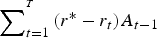
$$\sum\limits_{t = 1}^{^T} {(1 + r{^\ast})^{T - t} ({\rm AMT}_t - {\rm AMT}_{t}^{r:C} )} = \sum\limits_{t = 1}^T {(1 + r{^\ast})^{T - t} r{^\ast}({\rm UAL}_{t - 1}- {\rm UAL}_{t - 1}^{r:C} )}. $$

This answers the question, ‘How would cumulative amortization differ from the actual if investments had met the assumed return, and amortization had adjusted dollar-for-dollar to the interest on the resulting UALs?’ It is the counterpart to the ‘what if’ impact on UAL. It is represented in Fig. 5 as the $7.0 billion blue bar in the first column, atop the $5.0 billion red bar for the UAL impact. The total impact of the gap in investment returns – UAL plus cumulative amortization – is $12.0 billion under exogenous C _t .

Figure 5. Impact on UAL and cumulative amortization. C _t vs. α _t vs. AMT _t exogenous. Adapted from CSTRS, FY00–FY14.

The total impact is the same under exogenous AMT _t . Since there is no amortization impact under exogenous AMT _t , the $12.0 billion red bar for UAL impact in the third column is also the total impact. Thus, the difference between the red bars in the first and third columns of Fig. 5 (the UAL impacts) is equal to the $7.0 billion blue bar in the first column (the impact on cumulative amortization under exogenous C _t ).

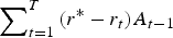
Further insight can be drawn from the explicit solution to the UAL impact under exogenous AMT _t , provided in the Appendix. As shown there, the UAL impact of the gap in investment returns is the compounded gap between (1 + r*) and (1 + r _t ) over the T-year period, as applied to the initial assets and annual cash flows. Recall that under exogenous C _t the UAL impact is $\sum\nolimits_{t = 1}^T {(r^{\ast} - r_t )A_{t - 1}} $ , i.e., essentially the uncompounded gap. The difference between the two follows from the SS assumption that amortization covers interest on the additional UAL, so there is no compounding. There is, instead, the cumulative impact on amortization.

For my preferred model, exogenous α _t , the total impact is also $12.0 billion, split between $7.3 billion on UAL and $4.7 billion on cumulative amortization, represented by the blue bar in the second column of Fig. 5. In short, the SS method implicitly attributes a substantial portion ($2.3 billion here) of the total impact of the gap in investment returns to amortization instead of UAL. That is, the SS method implicitly assumes that the gap in returns generates much more subsequent amortization than actual formulas would imply, so the UAL impact is that much smaller. More precisely, the SS counterfactual scenario is that without the gap, amortization would have been $7.0 billion lower, instead of the $4.7 billion implied by the amortization formula, so the UAL would have been only $5.0 billion lower, instead of $7.3 billion.

Similar observations apply to the impacts of liability losses (including benefit hikes) on the UAL and cumulative amortization. As shown in the Appendix, under exogenous AMT _t , the UAL impact includes the cumulative compound interest $\sum\nolimits_{t = 1}^T {(1 + r^{\ast})^{T - t} (L_t - L_{t \vert t - 1}^e )} $ , unlike the SS method where no interest accrues, $\sum\nolimits_{t = 1}^T {(L_t - L_{t \vert t - 1}^e )} $ . Again, that is because in the SS framework, with exogenous C _t , AMT _t responds to cover the interest on liability losses. With AMT _t exogenous, these losses have no impact on amortization. My preferred model, exogenous α _t , lies in between. Thus, the second triplet in Fig. 5 is similar to the first, but on reduced scale.Footnote ²³

One might be tempted to dismiss the impact on cumulative amortization as a matter of little significance since this has already been paid. But this impact is not totally benign. It means that some of the costs have been shifted from the cohort that incurred them to a later (albeit recent) cohort, creating some generational inequity in doing so. In other words, the split of the impact between paid (cumulative amortization) and yet-to-be-paid (UAL) is really a split between generational inequity already imposed and generational inequity to come. It is important to understand both of them. The SS method understates the impact of the gap in investment returns on UAL, by implicitly overstating the impact on cumulative amortization.

8 The liability impact of POBs

The SS method also provides a highly misleading account of POBs' impact on UAL. As noted above, if a state issues POBs to ‘pay down,’ say, $2 billion in a fund's UAL (as did CSTRS in 2008) the cumulative impact under the SS method remains at $2 billion every year thereafter.Footnote ²⁴ This is regardless of the returns – positive or negative, above or below r* – on the proceeds invested in the fund (let alone the outstanding POB debt incurred by the state).Footnote ²⁵

The math behind this is straightforward. Standard actuarial accounting adds the proceeds from any year's bond issue, POB _t , to the fund's assets, A _t , in (3), so the annual gain/loss statement (4) becomes:

(4 POB) $$\Delta _{t - 1,t} {\rm UAL} = (r{^\ast} - r_t )A_{t - 1} + (r{^\ast}{\rm UAL}_{t - 1} - {\rm AMT}_t ) + (L_t - L_{t \vert t - 1}^e ) - {\rm POB}_t, $$

and the SS method's multi-year accounting extends (5) to:

(5 POB) $$\eqalign{\Delta _{0,T} {\rm UAL} &= \sum\limits_{t = 1}^T {(r{^\ast} - {\rm} r_t )A_{t - 1} }+ \sum\limits_{t = 1}^T {(r{^\ast}{\rm UAL}_{t - 1} - {\rm AMT}_t ) }+ \sum\limits_{t = 1}^T {(L_t - L_{t \vert t - 1}^e ) }- \sum\limits_{t = 1}^T {{\rm POB}_t} \cr &= \Delta _{0,T} {\rm UAL}^{r:{\rm \Sigma}} + \Delta _{0,T} {\rm UAL}^{C{\rm :\Sigma}} + \Delta _{0,T} {\rm UAL}^{L:\Sigma} + \Delta _{0,T} {\rm UAL}^{{\rm POB:\Sigma}}.} $$

Thus, any proceeds from POBs in year t continue unchanged in Δ_0,T UAL^POB:Σ thereafter. Figure 6 shows the FY08 reduction in UAL from that year's POB and the SS method carries it forward as depicted in the flat line beyond FY08, Δ_0,T UAL^POB:Σ (this line was omitted from Fig. 1).

Figure 6. POB impact. SS, exogenous C _t , α_t  +  POB debt, CSTRS, FY00–FY14 adapted from CSTRS, supplemented by State of Connecticut Annual information statement.

There are three flaws in the method that underlie this result, two of which were discussed above, but not their implications for POB accounting. To see them in this context, it is helpful to note that Δ_0,T UAL^POB:Σ is the difference between the actual rise in UAL, Δ_0,T UAL, as given in the first line of (5 POB) and the SS counterfactual if the POB had not been issued:

(5 CF^POB ) $$\eqalign{\Delta _{0,T} {\rm UAL} = \sum\limits_{t = 1}^T {(r{^\ast} - {\rm} r_t )A_{t - 1}} + \sum\limits_{t = 1}^T {(r{^\ast}{\rm UAL}_{t - 1} - {\rm AMT}_t )} + \sum\limits_{t = 1}^T {(L_t - L_{t \vert t - 1}^e ) - 0},}$$

where the fourth term is zero, since there are no POBs in this counterfactual.

The first flaw is the SS method's exogenous treatment of the series of lagged asset values, A _{t −1}, in the first term above. As discussed earlier, this flaw had relatively minor implications for the other UAL-drivers, but it is more significant for the POB counterfactual. After all, the point of issuing a POB in period t was to add assets, so, in its absence, A _t would be lower – $2 billion lower in the case of CSTRS’ FY08 issue. Consequently, any losses due to subsequent gaps between the actual and assumed returns would be overstated in the SS counterfactual, since those assets would not have been there. The first term of (5 CF^POB ) should be lower, and the difference with (5 POB) – the measured impact – should be greater in algebraic value. To state the result directly, the POB's favorable UAL impact in period t is partially offset in t + 1 by the gap in returns on the proceeds, and similarly in following years. This effect is missed by the SS method's treatment of the lagged asset series as exogenous.

CSTRS provides a dramatic example. Immediately following the POB issue of $2 billion, the fund lost 17.84% in FY09, 26.34 percentage points below the assumed return. Thus, the gap in returns on the $2 billion was $527 million that year, offsetting a good portion of the prior year's UAL reduction from the POB proceeds. This can be seen in Fig. 6, on the dotted curve Δ_0,T UAL^POB:C, representing the POB's impact on UAL, with endogenous asset values (but still exogenous C). The effect of the FY09 investment loss on the POB's proceeds can be seen by comparing the point on that curve with the solid curve for Δ_0,T UAL^POB:Σ, lying along the −$2 billion line. It is certainly intuitive that the $2 billion reduction in UAL from the FY08 proceeds was attenuated in FY09 by the losses on those proceeds, but it is not reflected in the SS method, with exogenous A _t−1.

The second flaw underlying the SS method's flat Δ_0,T UAL^POB curve is the implicit amortization assumption that is the main subject of this paper – exogenous C _t , the second term of (5 CF^POB ). For exogenous α _t , the Δ_0,T UAL^POB:α curve lies below Δ_0,T UAL^POB:C , as shown in the dashed line of Fig. 6. Both curves reflect a cut in amortization payments triggered by the cut in UAL, but they are cut by less on Δ_0,T UAL^POB:α than on Δ_0,T UAL^POB:C . Under exogenous C _t , amortization payments are cut by an amount equal to the reduced interest on the UAL, but under exogenous α _t , they are only cut by a fraction of that amount, α _t . The net impact (beyond the initial $2 billion) under each assumption is the difference between the returns on the proceeds and the reduction in amortization. By FY14, the cumulative return on the proceeds, although less than r*, was large enough to offset the cut in payments under exogenous α _t , so the net reduction of UAL was greater than the initial $2 billion proceeds.

The third flaw is that standard UAL accounting omits the POB debt itself. To complete the picture for plans that have relied on POBs, one should integrate the POB debt into the UAL analysis. Although POBs are typically issued by the state, rather than the pension plan, for the taxpayer both the UAL and POB debt are liabilities.Footnote ²⁶ It is straightforward to add the outstanding POB debt to the POB impact on UAL. The result is depicted in the solid heavy blue line of Fig. 6, Δ_0,T UAL^POB:α  + POB debt. From the outset, the net liability has been increased, not decreased, by the POB. In addition to borrowing $2 billion for the CSTRS fund, the first 2 years of interest were also borrowed, as well as the issuing costs, for a total of $2.277 billion. Thus, for FY08, the net liability rose by $277 million. The net liability rises further in FY09, due to that year's large investment losses, reflected in Δ_0,T UAL^POB:α . In addition, the debt service is highly back-loaded, so the outstanding POB debt continues to rise (widening the gap between the heavy blue line and the dashed line).Footnote ²⁷ The net liability has drifted down since FY09, due to generally good investment returns, but remains in positive territory as of FY14: the POB debt of $2.333 billion outweighs my estimate of the UAL impact, −$2.088 billion.Footnote ²⁸

9 Additivity vs. interactions

A distinctive feature of the SS method is its additivity. As noted earlier, equation (5) (and its POB version, (5 POB)) provide a decomposition that adds up to the actual change in UAL. The alternative proposed here does not. Indeed, the first correction – endogenizing asset values – breaks additivity, even before replacing the amortization assumption. This can be seen in Fig. 1, where the sum of the dotted curves deviate (albeit only slightly) from the solid curves (which do add up), and when POBs are added in Fig. 6, the deviation is a bit greater.

The proposed alternative amortization assumption disrupts additivity more substantially. As Figs 4 and 5 show, adding up the UAL impacts under exogenous α _t can well exceed the sum under exogenous C _t (and the similar SS estimates) and, hence, the actual rise in UAL. As mentioned earlier, the reason is that there are large interaction effects, most notably between the gap in investment returns and the amortization formula (α _t  < 1). These interactions are intertemporal, rather than contemporaneous, which is why the multi-year decomposition is problematic, even if the annual gain/loss statement is not.Footnote ²⁹

What are we to make of the adding-up problem? ‘Not too much,’ in my view. The goal of a policy-relevant exercise is to evaluate useful counterfactuals, not to parcel out the rise in UAL in a fashion that adds up neatly. Indeed, if the solution adds up for faulty counterfactuals – often misunderstood – we misinform the user. If the user's interest is the impact of the gap in investment returns, we should use the right counterfactual to answer that question. That is, the policy-relevant question is ‘what has been the impact on UAL of the gap in investment returns, given the actual amortization formula?’ rather than the artificial version answered by the SS method: ‘what would have been the impact on UAL of the gap in investment returns if the amortization formula had covered interest?’ Additivity may be a short-hand way of indicating relative importance (X percent due to one factor and Y percent due to another), but if the price is assuming away important interactions, the effort is misguided. The relative importance of the UAL-drivers can be readily calculated from their individual impacts, including interaction effects. As noted earlier, CSTRS’ UAL impact from the gap in returns is about 50% greater than that of the contribution shortfall under exogenous C _t , but under exogenous α _t , it is about 125% greater – a big difference.