1. INTRODUCTION
Path planning for Unmanned Surface Vehicle (USV) navigation is a challenging problem due to the complexities of USV dynamics, environmental disturbances (Niu et al., Reference Niu, Lu, Savvaris and Tsourdos2016a), computational efficiency (Niu et al., Reference Niu, Lu, Savvaris and Tsourdos2016b), collision avoidance (Savvaris et al., Reference Savvaris, Niu, Oh and Tsourdos2014; Szlapczynski, Reference Szlapczynski2015) and timing constraints. Typical path planning algorithms can be classified into four categories: roadmap approaches, cell decomposition, potential fields and bug algorithms.
The goal of roadmap approaches is to reduce an N-dimensional configuration space to a set of one-dimensional paths for searching. These approaches attempt to capture free-space connectivity by constructing a graph. The roadmap approaches include the probabilistic roadmap method (Yuan et al., Reference Yuan, Liang, Fu, Xu and Ma2015), the rapidly exploring random tree (Kuffner and Latombe, Reference Kuffner and Latombe2000; Moon and Chung, Reference Moon and Chung2015), the expansive space planner (Hsu et al., Reference Hsu, Latombe and Motwani1997) and the random walk planner (Carpin and Pillonetto, Reference Carpin and Pillonetto2005; Lu et al., Reference Lu, Xu, Chen, Huang and Chen2016). Computational geometry-based methods comprise another branch of roadmap-based approaches, which include the Voronoi diagram (Wu et al., Reference Wu, Wen, Huang and Zhu2013) and the Visibility graph (Kaluder et al., Reference Kaluder, Brezak and Petrović2011; Zimmermann and Konig, 2016). Another category of path planning is cell decomposition (Iswanto et al., Reference Iswanto, Wahyunggoro and Cahyadi2016), which includes the exact and approximate cell decomposition approaches. The exact cell decomposition approach is also known as trapezoidal decomposition and comprises three main steps: (1) decomposing the free space into trapezoidal and triangular cells; (2) processing the adjacency relation between the cells; and (3) finally finding the optimal path. The approximate cell decomposition approach is also called the quadtree decomposition approach, which subdivides the mixed obstacle and free regions into four quarters and repeats the subdividing process iteratively. At a certain level of resolution, only the cells whose interiors lie entirely in the free space are used. Thereafter a graph-search algorithm can be directly applied to find a path from the starting point to the goal or target point, such as the well-known A* algorithm (Campbell et al., Reference Campbell, Naeem and Irwin2012). This solution has been evaluated for underwater obstacle avoidance experimentally (Phanthong et al., Reference Phanthong, Maki, Ura, Sakamaki and Aiyarak2014).
The potential field is popular mainly due to the low computational load it requires for trajectory generation and can hence produce trajectories in real-time. Moreover, planning and control are merged into one function and the potential field can be directly coupled to a control algorithm. However, the potential field method also has its drawbacks: it may be trapped in local minima in the potential field (Rezaee and Abdollahi, Reference Rezaee and Abdollahi2014). Due to this local minima limitation, it has mainly been used for local path-planning.
Finally, the bug algorithm and its variants are a category of path planning methods which assume limited knowledge of the environment. One example of the bug algorithm is the insect-inspired ‘bug’ algorithm, which assumes that only the direction to the goal is known and that local range measurement is available. This bug algorithm can be summarised in three steps: (1) heading towards the goal; (2) following obstacles until the vehicle can head towards the goal again; and (3) repeating the previous two steps until the goal is reached. The efficiency of the bug algorithm for robot path planning using range sensors was presented by Buniyamin et al., (Reference Buniyamin, Wan Ngah, Sariff and Mohamad2011). The bug algorithm is an obstacle avoidance method for local path planning (Loe, Reference Loe2008; Tam et al., Reference Tam, Bucknall and Greig2009; Lazarowska, Reference Lazarowska2015; Polvara et al., Reference Polvara, Sharma, Wan, Manning and Sutton2018).
The remainder of this paper is organised as follows: A literature review of the roadmap method is presented in Section 2. The problem of developing a path planning algorithm in complex geographic scenarios is presented in Section 3. The methodology of the proposed algorithm is described in Section 4. In Section 5, the proposed algorithm, Voronoi algorithm and the VM algorithm are compared in terms of total distance and computational efficiency. Finally, the Voronoi, VM and VV algorithms are evaluated in 2,000 Singapore missions for quantitative comparison. Section 6 concludes the paper.
2. LITERATURE REVIEW
This work focuses on the roadmap-based path planning approach. The advantage of using the Voronoi diagram as a roadmap, among which the Visibility graph prevails, is its efficiency. The Voronoi diagram can be constructed in just O(nlog(n)) time, where n is the number of the vertices and O notation is as used in Computer Science to describe the complexity of an algorithm in terms of the execution time or space required in the worst-case scenario. The fastest-known algorithm for constructing the Visibility graph takes O(n 2) time (Ghosh and Mount, Reference Ghosh and Mount1991) and has O(n 2) edges in the worst case. Since the Voronoi diagram has O(n) edges, searching a Voronoi diagram-based roadmap is much faster than searching a Visibility graph. Another advantage of the Voronoi diagram is that the constructed roadmap keeps the path as far away from the obstacles as possible; in contrast, the Visibility graph keeps the path as close to the obstacles as possible, since the Visibility graph uses the edges of the obstacles as candidate paths. However, the disadvantage of the Voronoi diagram is that the generated path may be far from optimal in terms of distance. Therefore, to take advantage of the computational efficiency of the Voronoi diagram, the generated path must be refined.
A general method for refining a path obtained from a roadmap-based on classical numerical optimisation techniques has been proposed (Kim et al., Reference Kim, Pearce and Amato2003). Dijkstra's search algorithm (Dijkstra, Reference Dijkstra1959) was proposed to determine an optimal path and the edges that are closer to the obstacles will be assigned higher costs. However, this method does not generate an optimal path, since the path is constrained to the edges in the roadmap. A B-Spline approximation method was used to improve the smoothness of the path obtained from the roadmap (Ibarra-Zannatha et al., Reference Ibarra-Zannatha, Sossa-Azuela and Gonzalez-Hernandez1994). In the work of Wein et al., (Reference Wein, Van den Berg and Halperin2007), a new diagram called the VV (C) diagram was proposed. The VV (C) diagram integrated the Visibility graph and the Voronoi diagram while also keeping the path away from the obstacle with a clearance distance c, which is a configurable value. However, as this algorithm is Visibility graph-based, the processing time is  $O(n^{2}log(n))$, which is impractical for large spatial datasets. In the work of Masehian and Amin-Naseri (2004), the Voronoi diagram, Visibility graph and potential field were integrated into a single architecture to provide a parametric trade-off between the safest and shortest paths, and the resulting generated paths were shorter than in the Voronoi and potential field methods and faster than in the Visibility graph. However, this algorithm is very complicated and still contains bumps and rudimentary turns; hence, the algorithm is not ideal for USVs in dynamic environments. A VM (Voronoi shortest path refined by Minimising the number of waypoints) algorithm was proposed by Bhattacharya and Gavrilova (Reference Bhattacharya and Gavrilova2008). The generated path was ultimately smoothed by using a corner-cutting technique. It was demonstrated that the proposed algorithm reduced the length of the Voronoi path and still kept the computational efficiency as low as O(nlog(n)). Another rapid path re-planning algorithm was proposed by Candeloro et al., (Reference Candeloro, Lekkas and Sørensen2017) based on the Voronoi algorithm. However, the path generation was limited to only the edges of the Voronoi diagram.
In this work, a new algorithm, named the Voronoi-Visibility (VV) algorithm, is proposed that combines the Voronoi diagram and the Visibility graph, taking advantages of the strengths of each to produce an optimal solution in terms of safety navigation, path distance and computational cost. To benchmark its performance, the proposed algorithm was compared with the VM algorithm in terms of path length and computational time.
3. PROBLEM STATEMENT
Research on path planning algorithms for USVs to operate in complex geographical scenarios has mainly focused on two challenges: ensuring high computational efficiency in processing large spatial datasets and maintaining clearance distances from obstacles, such as island coastlines.
3.1. Large spatial dataset
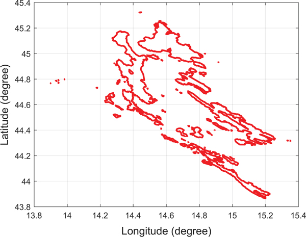
A detailed high-resolution navigation chart would improve the accuracy of the path planning result but also creates a computational burden. For example, there are 98 islands in the Singapore Strait and 114 islands along the included Croatian coastline, as shown in Figures 1 and 2, respectively. By querying high-resolution island data for the Singapore Strait, it was found that there were around 4,128 vertices for representing the Singapore islands. Considering the large number of vertices, even the fastest Visibility graph algorithm would incur a computational cost of O(n 2) time and an edge number of O(n 2) in the worst case. Each segment must be checked to determine whether it intersects with any island coastline, such that processing such a large amount of data would increase the roadmap construction time and path searching time significantly. It is therefore impractical to use the Visibility graph directly due to its inefficiency.
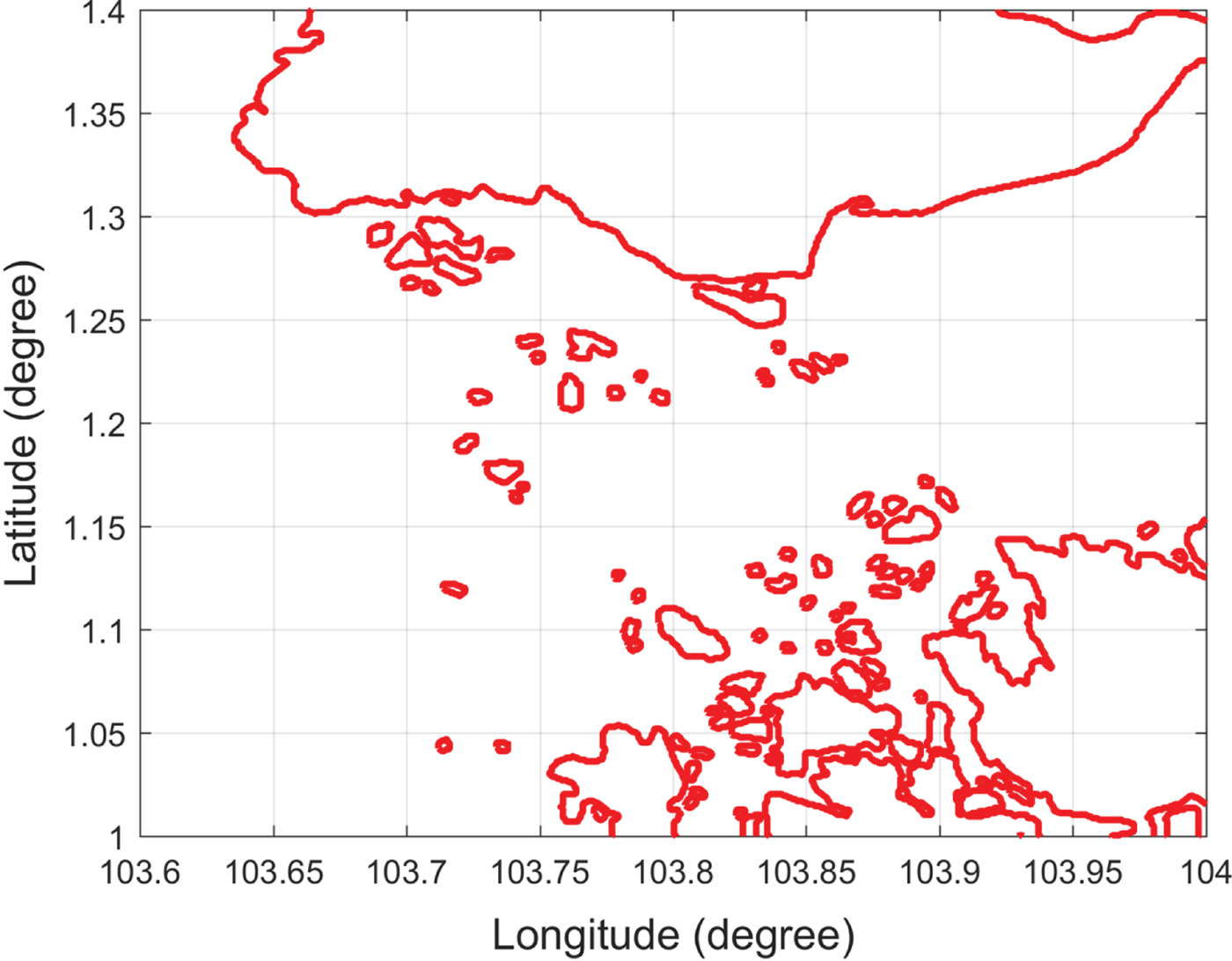
Figure 1. Singapore islands.
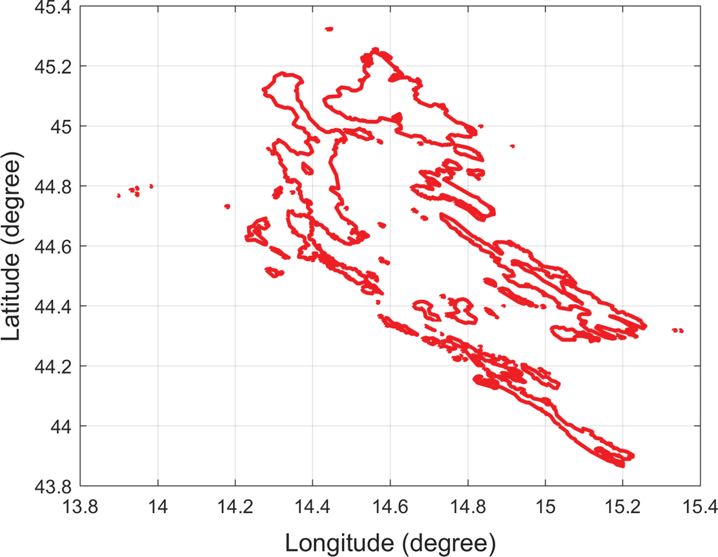
Figure 2. Croatia islands.
3.2. Clearance distance
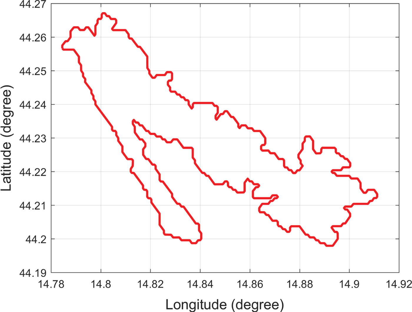
Map data may occasionally be inaccurate. Figure 3 shows an example of a Croatian island representing data obtained from the Global Self-Consistent Hierarchical High-Resolution Shorelines (GSHHS) dataset. However, an overlay of the island data onto a Google map (Figure 4) shows inconsistent profiles among the different map providers. The average distance between the two coastline profiles was around 200 metres. Accordingly, path planning algorithms should account for the problem of map inaccuracy when keeping the USV away from island coastlines with a safe clearance distance, and the clearance distance can also keep the USV away from crowded environments near coastlines.

Figure 3. Croatian island.
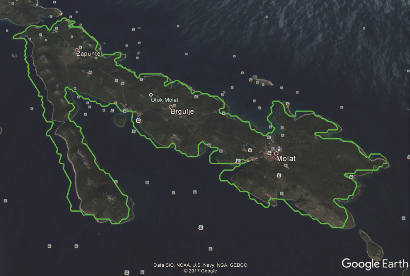
Figure 4. Illustration of data inaccuracy on a Croatian island.
4. METHODOLOGY
The methodology of the proposed algorithm is presented in this section, which is organised as follows: Section 4.1 summarises the architecture of the proposed algorithm. Section 4.2 presents the environmental dataset used in the research. The Voronoi collision-free roadmap generation is described in Section 4.3, while the Voronoi shortest path generation is presented in Section 4.4. Next, the Visibility graph generation approach is presented in Section 4.5. Finally, the combined VV algorithm is introduced in Section 4.6.
4.1. Algorithm architecture
The architecture of the proposed VV approach is shown in Figure 5. This algorithm includes four parts: collision-free Voronoi roadmap generation, Voronoi-based path planning, Visibility graph generation and VV path planning.
Figure 5. The architecture of the VV path planning algorithm.
In the collision-free Voronoi roadmap generation stage, coastlines are expanded by the coastline expanding algorithm, and the expanded coastlines keep the subsequently generated roadmap at a clearance distance c from the original coastlines. The expanded coastline data are then processed by the Voronoi diagram method and the unreachable paths are removed, which produces the collision-free Voronoi roadmap. In the Voronoi shortest path generation stage, the starting point and the destination are inserted into the Voronoi roadmap and Dijkstra's search algorithm is applied to generate the Voronoi shortest path. In the Visibility graph generation stage, the Voronoi shortest path is processed using the Visibility graph. Finally, Dijkstra's search algorithm is again applied to search for the VV shortest path.
4.2. Environmental dataset
In this paper, full-resolution (f) data from the Global Self-Consistent Hierarchical High-Resolution Shorelines (GSHHS) dataset are used. The full-resolution dataset has the highest resolution level among those from the GSHHS, including high-resolution (h), intermediate-resolution (i), low-resolution (l) and crude-resolution (c). The resolution is less than 100 metres. Real navigation data not only provide a real simulated environment but can also be used to demonstrate the efficient computing capability of the proposed algorithm.
4.3. Voronoi roadmap generation with clearance c
Collision-free Voronoi roadmap generation includes three steps: (1) expanding the coastlines, (2) applying the Voronoi diagram algorithm and (3) removing the unreachable paths.
4.3.1. Coastline expanding algorithm
To ensure the safety of the USV, each island coastline is expanded by c metres, which is configurable and can be specified by the users depending on their requirements.
The coastline expanding algorithm was realised by calculating the position of each expanded coastline endpoint. In Figure 6, the coastline A−B−P is expanded to a−b−p, and the expanding distance is c metres. The segment A−B is parallel to the segment a−b, and their distance is c metres. The segment B−P is parallel to the segment b−p, with a distance of c metres. The positions of points A, B and P are denoted by  $A(x_{A},y_{A}),B(x_{B},y_{B})$ and P(x P, y P), respectively.

Figure 6. Coastline expanding algorithm.
To determine the expanded line segments a−b−p, the expanding algorithm needs to calculate the position of b(x b, y b). The angle bisector of angle θABP is denoted by line bo. The Line-Of-Sight (LOS) angle of line bp is denoted by θpbm and the LOS angle of line ba is denoted by θabm.
First, θabm and θpbm are calculated using Equations (1) and (2), respectively:
 $$\theta_{abm}=\hbox{atan}\left(\displaystyle{y_{a}-y_{b} \over x_{a}-x_{b}} \right)$$
 $$\theta_{pbm}=\hbox{atan}\left(\displaystyle{y_{p}-y_{b} \over x_{p}-x_{b}} \right)$$
The angle θobp and the length of Bb are calculated using Equations (3) and (4), respectively:
 $$\theta_{obp}=\displaystyle{\theta_{abm}-\theta_{pbm} \over 2}$$
 $$\vert Bb \vert = \displaystyle{c \over sin(\theta_{obp})}$$
Next, position b(x b, y b) is calculated by Equations (5) and (6), respectively:
 $$x_{b} = x_{B} - \vert Bb \vert \times \cos (\theta_{obp} + \theta_{pbm})$$
 $$y_{b} = y_{B} - \vert Bb \vert \times \sin (\theta_{obp} + \theta_{pbm})$$
Using the coastline expanding algorithm, all the expanded coastline point positions can be calculated in O(n) time. Figure 7 shows an example of expansion with one of the Singapore islands. The expanded distance is c=200 m.
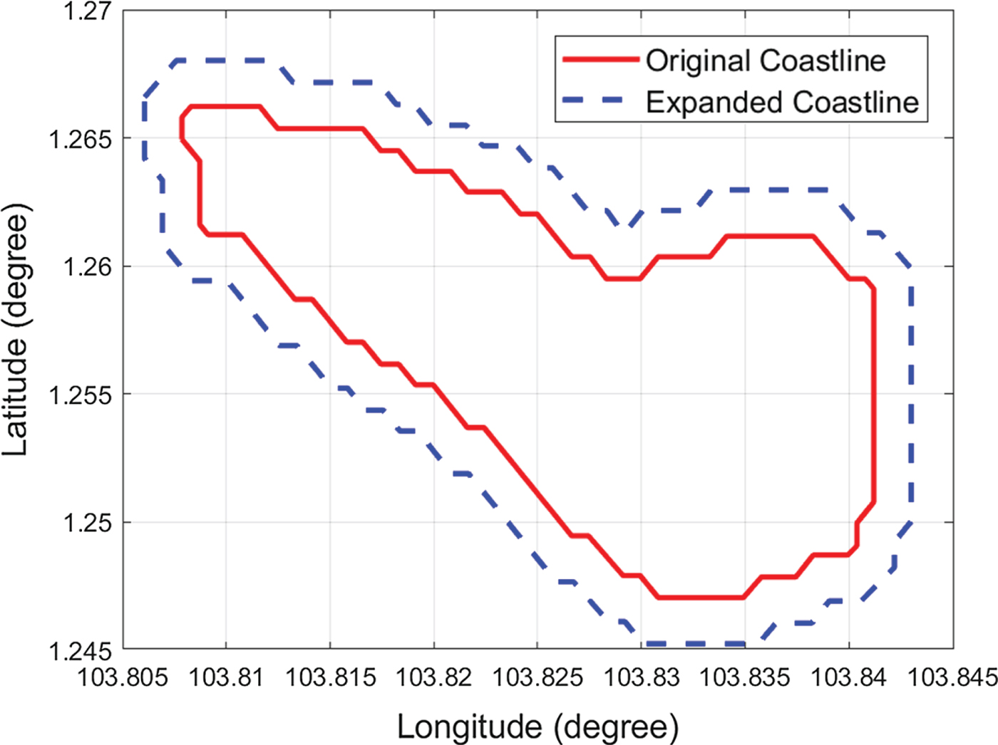
Figure 7. Illustration of coastline expanding algorithm.
4.3.2. Voronoi roadmap generation
The Voronoi roadmap was built in O(nlog(n)) time. For implementation, the Delaunay triangulation should be created first, after which the Voronoi diagram should be generated from it. The procedure has been included in the built-in MATLAB function ‘voronoin’; the voronoin function can be expressed in Equation (7):
 $$[v,ce]=voronoin(x, y)$$
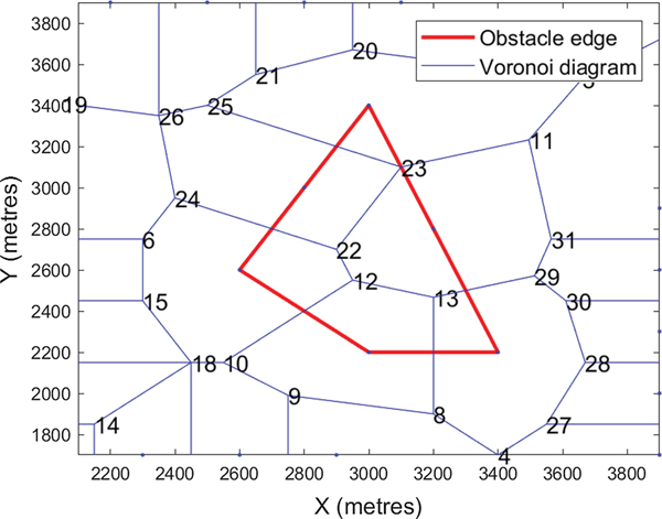
where the inputs x and y represent the longitude and latitude of all the coastline points, respectively. Outputs v and ce store the Voronoi node information and Voronoi cell information, respectively. By processing v and ce, the adjacency matrix F can be obtained. The edge weights for any connected pair of node i and node j, denoted as F(i, j) and F(j, i), are equal to 1. Unconnected pairs will have edge weights of 0. Figure 8 depicts the Voronoi diagram of an obstacle.

Figure 8. The Voronoi diagram of a polygon.
4.3.3. Removing unreachable paths
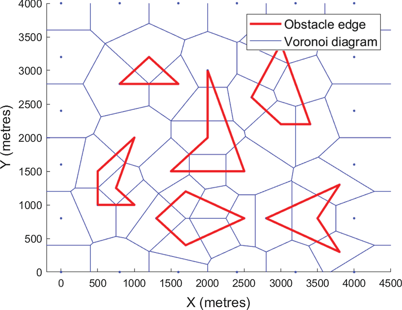
In Figure 8, segments 23–11, 23–25, 23–22, 22–24, 12–22, 12–10, 12–13, 13–8 and 13–29 are not reachable because they cross obstacles. Two types of paths must be removed: (1) path segments that intersect with the coastlines, and (2) paths that are connected to those nodes that fall inside the island profile.
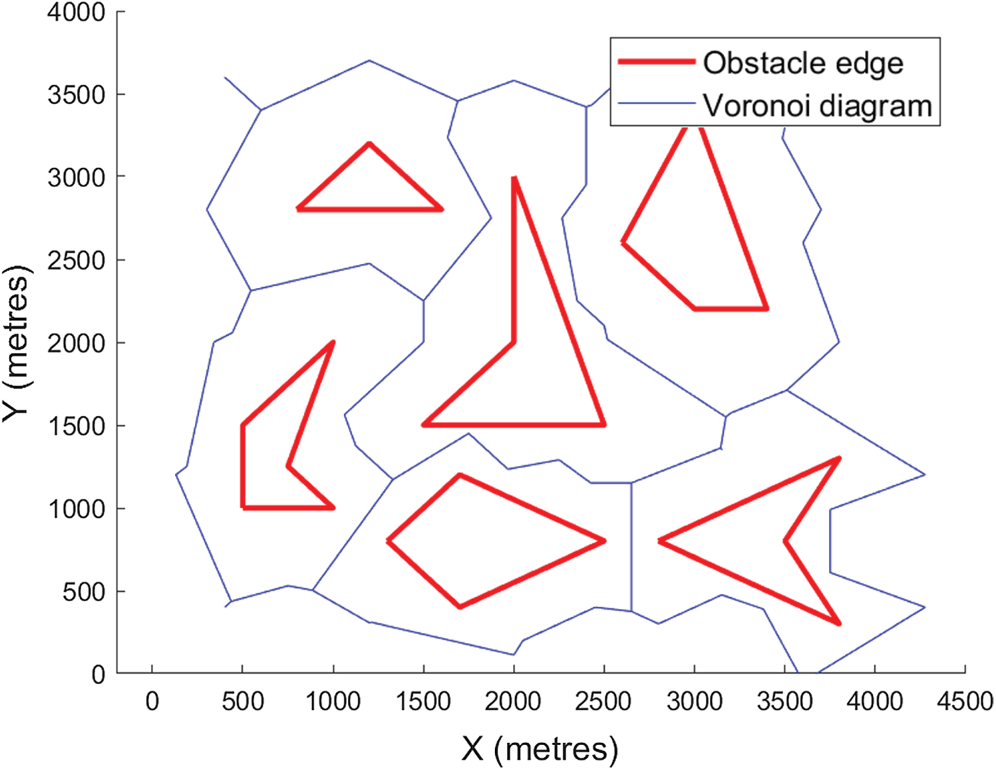
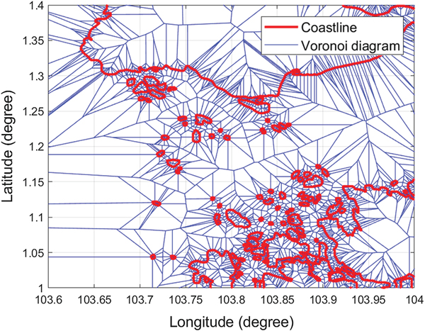
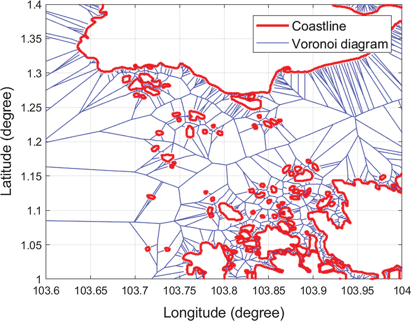
Voronoi diagrams of obstacles and Singapore islands are shown in Figures 9 and 11, respectively. When unreachable paths are removed, the roadmap becomes much clearer, as shown in Figures 10 and 12. Since checking the clearance of one Voronoi edge needs O(log(n)) time and the Voronoi diagram has O(n) edges, removing all unreachable paths requires O(nlog(n)) time. The adjacency matrix F must be updated accordingly. Assuming a removed path ij, the values of F(i, j) and F(j, i) will be updated to 0.

Figure 9. Voronoi roadmap of polygon obstacles.

Figure 10. Collision-free roadmap of polygon obstacles.

Figure 11. The Voronoi roadmap of Singapore islands.

Figure 12. Collision-free roadmap of Singapore islands.
4.4. Voronoi shortest path generation
4.4.1. Insertion of starting point and destination
Assuming there are N nodes generated by the Voronoi diagram, the starting point and the destination point are added to the Voronoi nodes as node N+1 and node N+2. Matrix F is then expanded from size N×N to size  $(N+2)\times (N+2)$. The nearest reachable Voronoi nodes to the starting point and destination point are denoted as node N+1 and node N+2, respectively.
4.4.2. Dijkstra's search algorithm
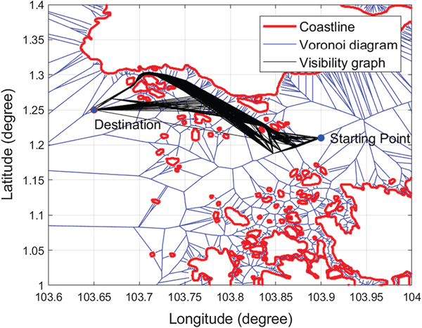
The element of matrix F should be changed from 1 to the Euclidean distance of the two corresponding nodes, as shown in Table 1, where S denotes the closest Voronoi node to the starting point node N+1, D denotes the closest Voronoi node to the destination point node N+2, L represents the length between two nodes, for example, L S, N+1 represents the length between S and N+1. Dijkstra's search algorithm is then applied to search for the shortest path from node N+1 to node N+2. Assuming the starting point is (103·9, 1·21) and the destination point is (103·65, 1·25), the path produced by Dijkstra's search algorithm is shown in Figure 13. It can be seen that the Voronoi shortest path is far from optimal and it must be refined.
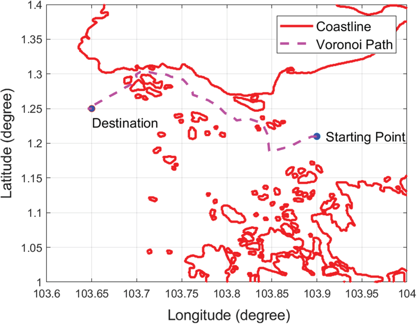
Figure 13. Voronoi shortest path.
Table 1. The adjacency matrix F with length information.

4.5. Visibility graph generation
To refine the Voronoi shortest path, the Visibility graph is applied. A waypoint is denoted as w i on the Voronoi shortest path, where (i={1 .. m}) and m is the number of waypoints. It must first be verified whether the line segment w iw 1 has an intersection with the expanded coastlines. If there is no intersection, the adjacency matrix will be updated by F i, 1=L i, 1. The same operation is repeated with all line segments in the roadmap by two nested loops (see the pseudocode shown in Figure 14).

Figure 14. The pseudocode of the Visibility graph.
The Visibility graph has O(m 2) edges, and the construction of the collision-free Visibility graph requires  $O(m^{2}log(n))$ time. After applying the Visibility graph algorithm, the VV roadmap is obtained, as shown in Figure 15. The Visibility graph generates more possible paths to the Voronoi roadmap, which changes the path topology; for example, a path sailing on a different side of an obstruction may occur in VV.

Figure 15. VV roadmap.
4.6. Voronoi-Visibility shortest path generation
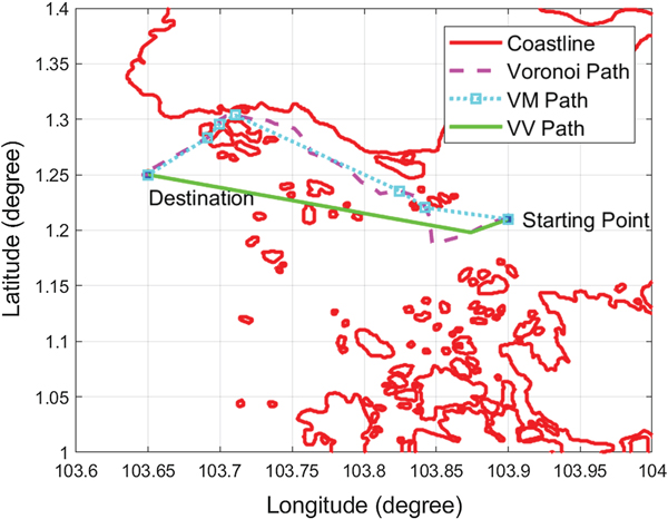
Dijkstra's search algorithm is applied again to search for the shortest path from the VV roadmap. The Voronoi and VV shortest paths are shown in Figure 16(a). It is found that the VV path is 27·24% shorter than the Voronoi path. In addition to having a shorter distance, the produced path also meets the safety condition of clearance distance from the expanded coastlines. To illustrate the effectiveness of the safety condition, Figure 16(b) shows a detailed, enlarged view of a small region in Figure 16(a) (the blue box). The VV path maintains the clearance distance from the original coastlines, meaning that the path generated by the proposed algorithm is safe for the USVs to operate in.
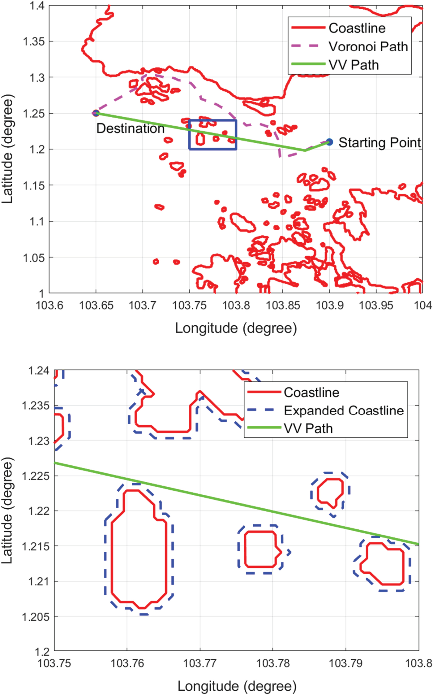
Figure 16. VV and Voronoi shortest paths.
5. NUMERICAL SIMULATION
5.1. Voronoi diagram-based path planning algorithm for comparison
For comparative purposes, the VM path planning algorithm was assessed against the proposed method. The rationale for choosing the VM algorithm for comparison was that the VM is considered one of the main authentic solutions in this area. As in the proposed algorithm, in VM, the coastlines are first expanded, after which the starting point and destination point are inserted into the roadmap. Dijkstra's search algorithm is then applied to search for the shortest path between the starting point and the destination point. The difference between the VV and VM algorithms is that once the Voronoi shortest path is generated, the VM algorithm will refine the path by minimising the number of waypoints on the Voronoi path instead of applying the Visibility graph and Dijkstra's search algorithm.
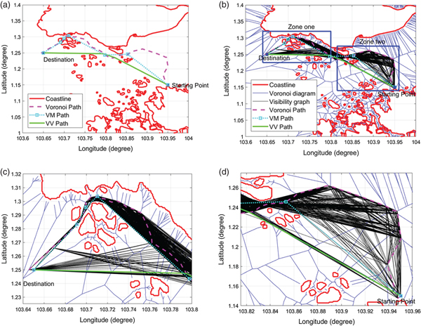
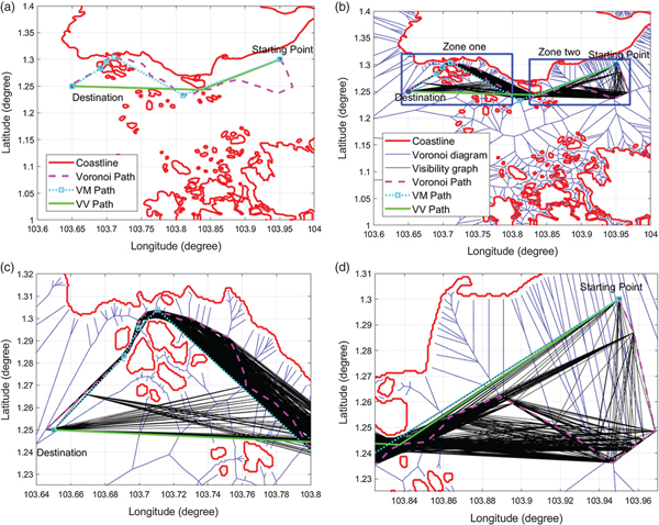
The procedure for minimising the number of waypoints is as follows: For a waypoint w i on the Voronoi shortest path  $(i=\{1\,..\,m-2\})$, where m is the number of waypoints on the Voronoi shortest path, the line segment w iw i+2 is checked to determine whether it has an intersection with the expanded coastlines. If not, then w i+1 is removed from the shortest path, and the process is repeated from waypoint w i+2. If so, then w i+1 is retained and considered the next waypoint for processing. The Voronoi, VM and VV shortest paths are shown in Figure 17. Here, it is shown that the VV shortest path saves 12·76 % more of the total length than does the VM path. Figure 18 shows the Voronoi, VM and VV shortest paths with the Voronoi diagram and the Visibility graph in the background. The Visibility graph generates more available paths and makes it possible for the USV to travel on another side of the islands, hence saving path length when compared to the VM algorithm.

Figure 17. Comparison of Voronoi, VM and VV shortest paths.
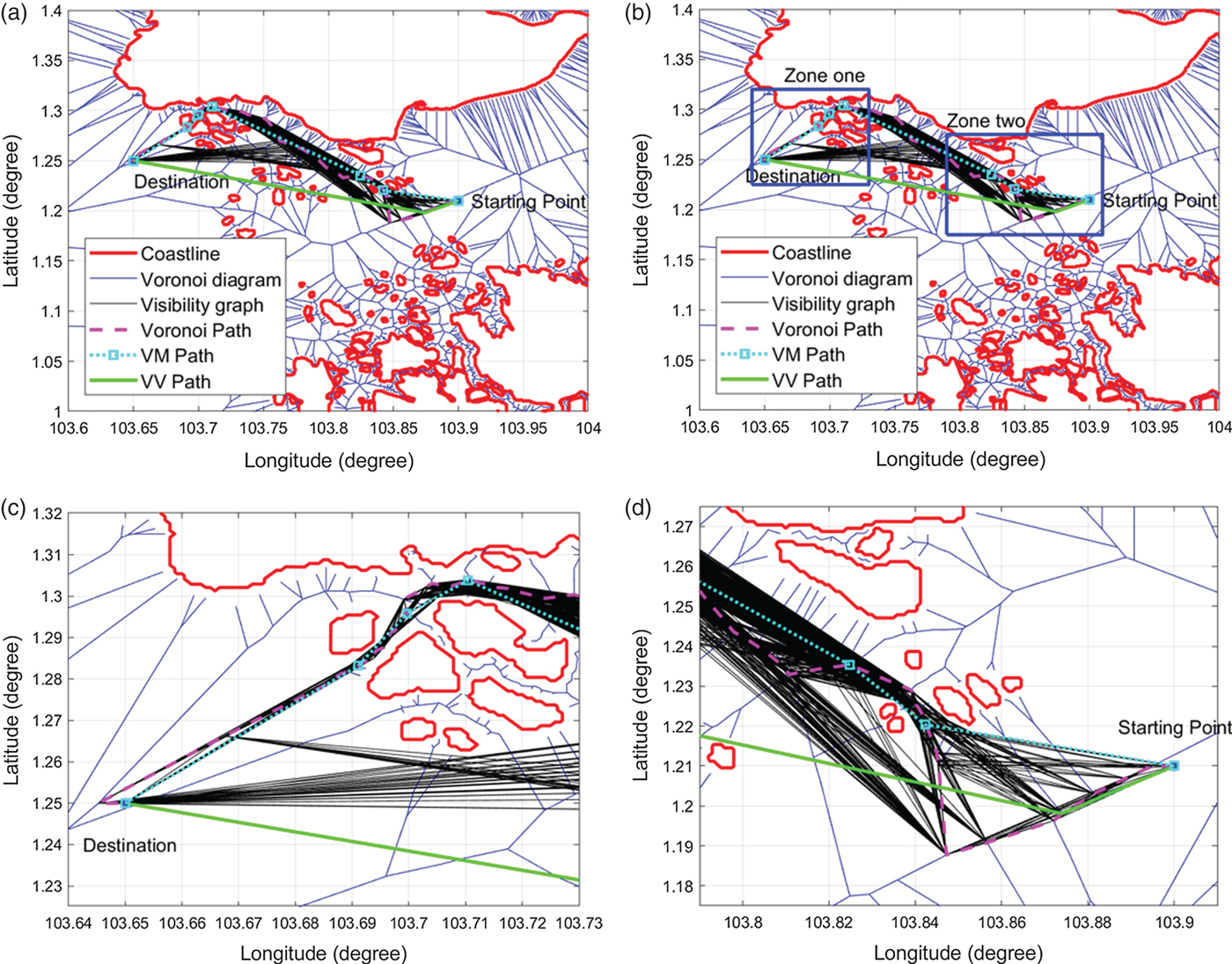
Figure 18. Comparison of Voronoi, VM and VV shortest paths (In (b), zone one and zone two are represented by blue rectangles, which are zoomed in (c) and (d)).
5.2. Ten USV mission scenarios in Singapore
All the simulations were carried out on a 2·7 GHz Intel Core i7-6820HK processor with 16·0 GB RAM. The programmes were implemented using Matlab R2016b. In this stage, the proposed VV algorithm was compared with the VM algorithm for ten Singapore mission scenarios in terms of path length and computational time.
5.2.1. Path length comparison
The comparison of the path lengths is shown in Table 2. The clearance distance was set to be 100 metres. Each mission had different starting and destination end-points. The path length saved varied from 5·84% to 13·38%. The Voronoi, the VM and the VV shortest paths of Missions No. 3 and No. 10 are shown in Figures 19 and 20, respectively. It can be seen that the Voronoi shortest paths are far from optimal: although the VM path planning algorithm refined the Voronoi shortest path, in terms of path length, its performance was not as good as the proposed VV path planning algorithm.

Figure 19. The comparison of Voronoi, VM and VV shortest paths in Singapore Mission No.3 (In (b), zone one and zone two are represented by blue rectangles, which will be zoomed in (c) and (d)).
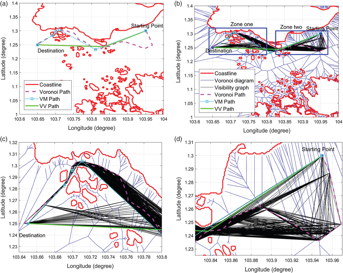
Figure 20. The comparison of Voronoi, VM and VV shortest paths in Singapore Mission No.10 (In (b), zone one and zone two are represented by blue rectangles, which will be zoomed in (c) and (d)).
Table 2. The comparison of the VV and VM algorithms in ten Singapore missions.
5.2.2. Computational time comparison
The computational times of the Voronoi, VM and VV algorithms were compared. As shown in Table 3, the Voronoi algorithm needed the least computational time. The VM approach costs more time than the Voronoi algorithm, which was less than 0.1 second, and the VV algorithm needed the longest time. Comparing the computational time between VV and VM, it was found that the extra computational time was less than 2.2 seconds. The extra computational time was proportional to the number of waypoints on the Voronoi path. Because the complexity of the fastest way to build the Visibility graph is O(n 2), the Visibility graph was applied to the Voronoi shortest path, whose vertices number m between 44 and 107, instead of being applied to the entire map, whose vertices number 4,128. Note that the code implemented in this research did not include any optimization technique to accelerate the computation. Moreover, according to the simulations of Bhattacharya and Gavrilova (Reference Bhattacharya and Gavrilova2008), when applying the Visibility graph to a map with 1,866 vertices, the computational time will be longer than 60 seconds. However, the computation time with the proposed VV algorithm ranges from 0.784 seconds to a maximum of 2.179 seconds, corresponding to 9.5% to a maximum 26% of extra time. The proposed VV algorithm therefore maintained the same level of computational efficiency as the Voronoi path planning algorithm.
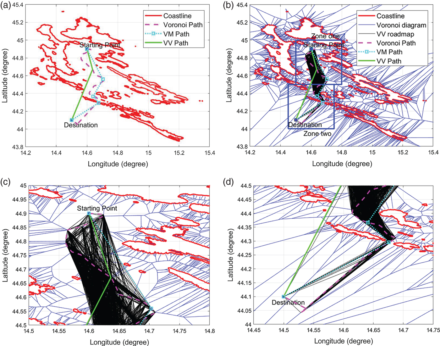
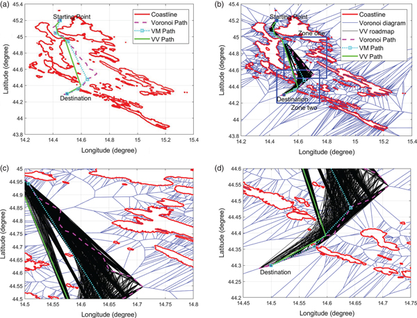
Figure 21. The comparison of the Voronoi, VM and VV shortest paths in Croatian Mission No.3 (In (b), zone one and zone two are represented by blue rectangles, which are zoomed in (c) and (d)).

Figure 22. The comparison of the Voronoi, VM and VV shortest paths in Croatian Mission No.4 (In (b), zone one and zone two are represented by blue rectangles, which are zoomed in (c) and (d)).
Table 3. Computational time comparison of the Voronoi, VM and VV shortest path planning algorithms in the Singapore missions.
5.3. Five USV mission scenarios in Croatia
To test the performance of the proposed algorithm in different spatial scenarios, the proposed algorithm was compared with the VM algorithm in five Croatian mission scenarios, as shown in Table 4. The saved distance was between 0.64% and 10.47%. The clearance distance was again set to 100 metres. The results of the three algorithms for Missions No. 3 and No. 4 are shown in Figures 21 and 22, respectively. It can be seen that the proposed VV algorithm still saves travelling distance when compared with the VM algorithm in the Croatian scenario, which demonstrated the flexibility of the proposed algorithm in dealing with different geographical scenarios. Table 5 shows the computational time of the three algorithms. The time difference between the VV and VM algorithms is proportional to the number of waypoints on the Voronoi path, which is between 9.260 seconds and 18.877 seconds. The time difference between the VV and VM algorithms in Croatia is longer than in the Singapore scenario because the Croatia scenario has a longer island coastline than Singapore and the number of Croatian island vertices is 12,022, which is about three times that of Singapore island vertices. According to the simulations of Bhattacharya and Gavrilova (Reference Bhattacharya and Gavrilova2008), the Visibility graph algorithm will take more than 60 seconds in the case of 1,866 vertices, while the proposed algorithm will take around 60 seconds in the case of 12,002 vertices, thus making the latter more computationally efficient than the former.
Table 4. The comparison of the VV and VM algorithms in five Croatian missions.

Table 5. Computational time comparison of the Voronoi, VM and VV algorithms in Croatian missions.

5.4. Two thousand mission simulations in Singapore
In order to quantitatively analyse the influence of spatial factors, such as homogeneities of island distributions, on algorithm performance, a total of 2,000 missions were simulated with random missions in two sub-regions of the map. In each sub-region, 1,000 pairs of random starting points and destinations were selected, as shown in Figures 23(a) and 23(b), respectively. Note that because the proposed algorithm was designed to deal with complex spatial scenarios, the randomly generated start points and destinations were only considered valid if the waypoint number with the VM algorithm was greater than one (excluding the starting point and destination). In other words, cases in which the direct paths between the start and end points were free of obstacles were excluded from the analysis. In case one, the inter-island distances varied more significantly than in case two, because the spatial domain of case one was a mixture of close and far islands, while the inter-island distance was more homogeneous in case two.
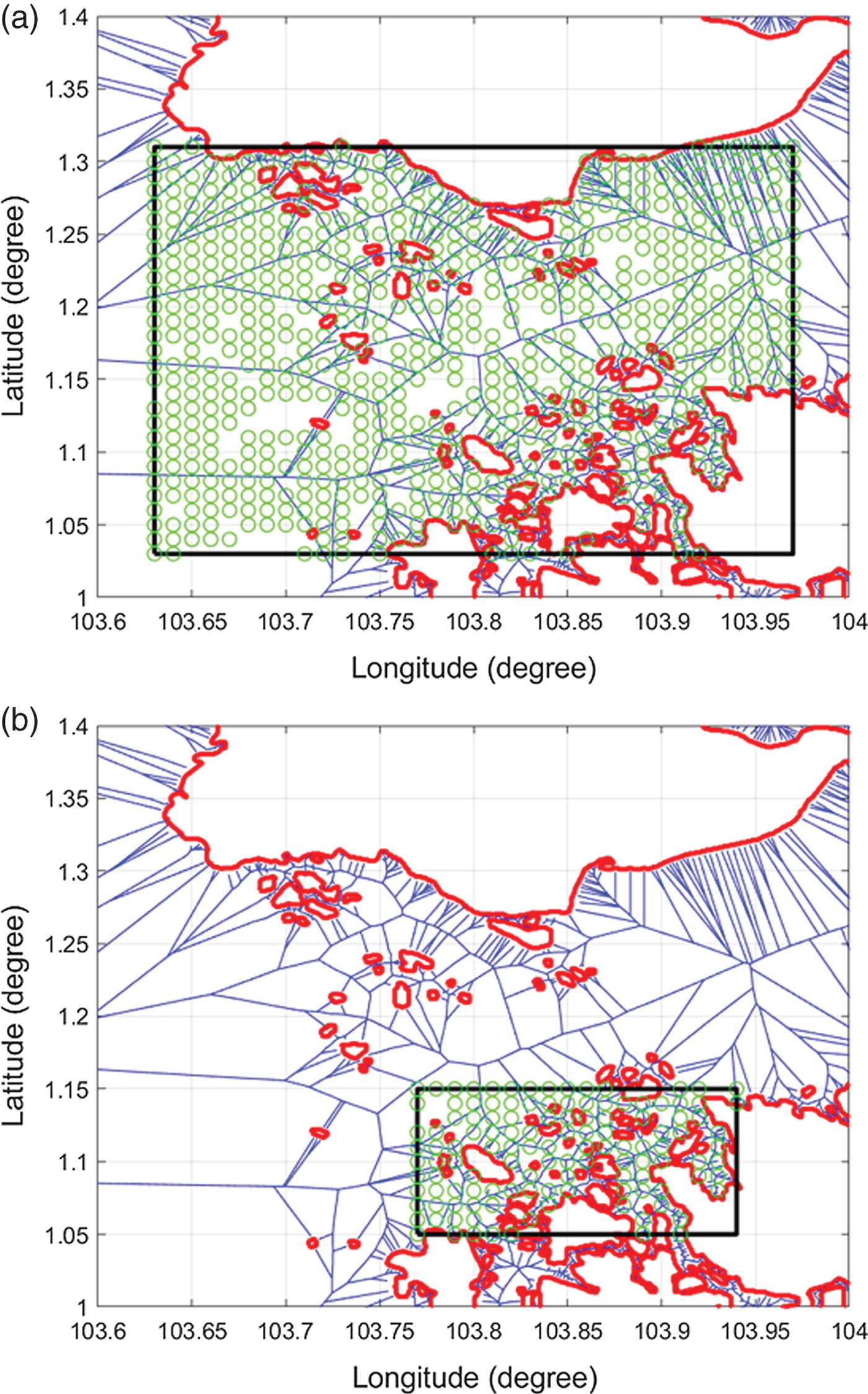
Figure 23. Mission area in case one (a) and case two (b) (Green circles are randomly selected start points and destinations).
The results are statistically represented in Figures 24 (case one) and 25 (case two). In case one, the path distance was 20%–25% shorter with the proposed VV method in 212 missions than with the Voronoi algorithm and 15%–20% shorter with VV in 143 missions than with the Voronoi algorithm. Overall, the proposed VV path saved more than 20% of the total length compared to the Voronoi path in 78% of the 1,000 missions in case one and saved more than 5% of the total length compared with the VM algorithm in 56% of the 1,000 missions. In Figure 25, VV saves more than 20% of the total length compared with the Voronoi path in 77.2% of the missions and saves more than 5% of the total length compared with the VM algorithm in 34.7% of the missions. Comparing the results of Figure 24(b) and 25(b), it can be concluded that the VV algorithm has a higher probability to save more distance in the case of a mixture of close and far islands than the case with homogeneous distance islands. Among these 2,000 missions, the length of VV will be the same as that of the VM algorithm in the worst case. However, the VM path is a subset of the VV roadmap, so that the VV path will never be longer than the VM path when applying Dijkstra's algorithm to search for the shortest path in the VV roadmap.
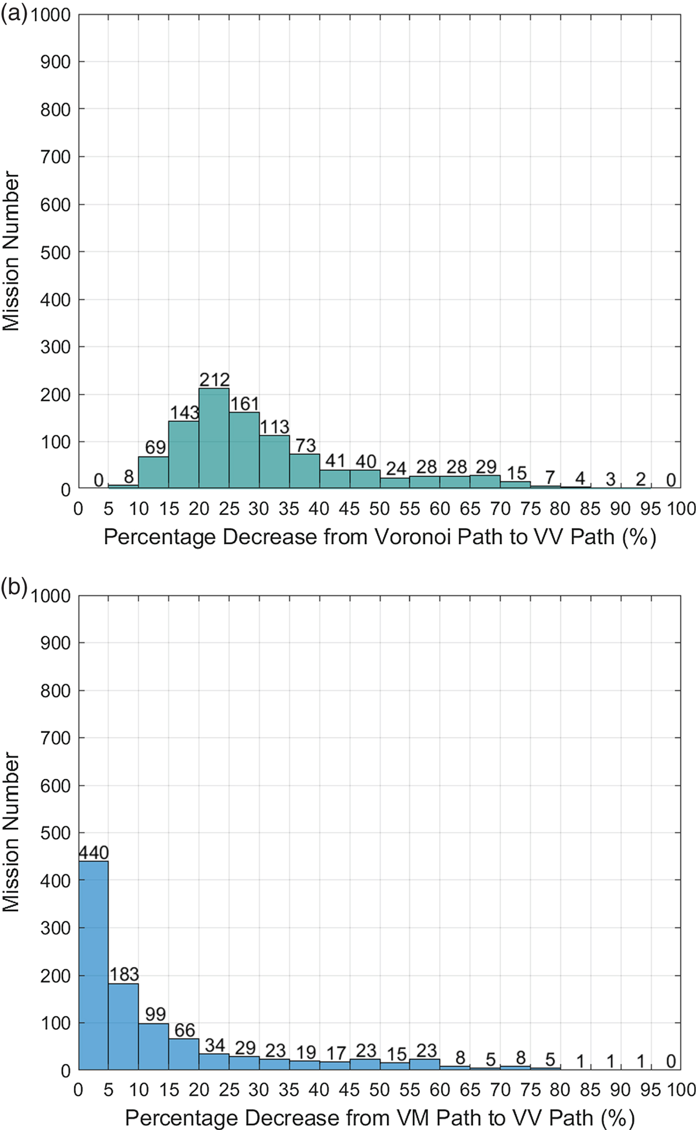
Figure 24. Comparison of Voronoi, VM and VV paths in case one.
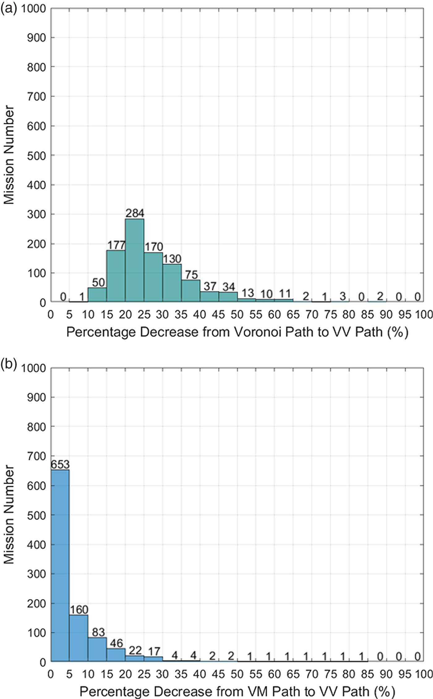
Figure 25. Comparison of Voronoi, VM and VV paths in case two.
6. CONCLUSION
In this paper, the coastline expanding algorithm, Voronoi diagram, Visibility graph and Dijkstra's search algorithms were integrated to solve the problem of USV shortest path planning. By comparing the path length and the computational efficiency of the proposed VV algorithm with that of the VM algorithm in the Singapore Strait missions and the Croatian islands missions, it can be concluded that the proposed algorithm generates shorter paths than the VM algorithm and maintains the same level of computational efficiency as that of the Voronoi shortest path planning algorithm. Two thousand mission simulations were carried out, together demonstrating considerable performance improvement with the proposed algorithm, especially in the case of a mixture of islands with large inter-distance variations rather than those of islands with more homogeneous distributions. In this work, the proposed algorithm addressed the least distance path planning problem, which can be extended in future work by modifying the adjacent matrix using time consumption weights or energy consumption weights considering the sea current data to solve the problem of least time or least energy path planning.