


1. INTRODUCTION
The conception of a ship domain is one of the vital terms of today’s sea navigation. Historically the first domain had a shape of a circle. The distance at the closest point of approach (DCPA) and the time remaining to reach this point (TCPA) are two parameters that are still used extensively in collision avoidance systems. This is in fact equivalent to applying a circle-shaped domain whose radius is the smallest acceptable distance between two ships. The next major steps in the development of the ship domain have been the Fuji model [Reference Fuji and Tanaka3] – an ellipse and the Goodwin model [Reference Goodwin4] – three segments of the circles of different radii for three sectors of the area surrounding the ship. These models have taken into consideration the course of a ship and international sea regulations respectively. The subsequent models by Davis [Reference Davis, Dove and Stockel2] and Coldwell [Reference Coldwell1] have brought back the regular shape of the domain (a circle and an ellipse) but the geometrical centre of the domain has no longer been identical to the position of an own ship. The domain according to Smierzchalski [Reference Smierzchalski15, Reference Smierzchalski16] has a shape of a hexagon whose dimensions take into account three sectors of the ship’s surroundings.
The simplicity of the circle-shaped domain, in comparison to the relatively complex subsequent models, was one of the factors leading to its continuous development. The associated parameters, DCPA and TCPA, have been further investigated. The key equations of collision avoidance manoeuvres and manoeuvres of required approach parameters were derived by Lenart [Reference Lenart6–Reference Lenart10]. There has been an expansion of the fuzzy domain [Reference Pietrzykowski13]. The threshold-based decision criteria – acceptable or unacceptable risk of collision (domain violated or not) are no longer sufficient for modern collision avoidance systems. In the face of difficulties in the direct measurement of the collision risk, indirect methods keep evolving, one of these being the measurement of the probability of the ‘safety failure’ situation [Reference Pietrzykowski and Gucma12, Reference Pietrzykowski and Gucma14]. At the same time new measures and indicators of risk are being created, of which some are based on the old parameters DCPA and TCPA [Reference Hwang5, Reference Lisowski11].
This paper introduces a new, simple measure of safety of the given situation, derived from the concept of a ship domain. It is especially useful when there is a significant risk of the domain violation and thus – considerable probability of a dangerous situation. The rest of the paper is organized as follows. Section 2 is a presentation of the measure: its definition, derivations of the formulas for Fuji domain model and a simulation example. In Section 3 a numerical algorithm that finds the measure value for any given ship domain is provided. Section 4 describes a method of determining the collision-avoidance manoeuvre that utilizes the measure presented. Section 5 discusses how the measure may be applied to already known formulae for collision risk. Finally, the conclusions are presented in Section 6.
2. THE PROPOSED MEASURE OF COLLISION RISK
The main reason why the term DCPA is still commonly used, is that it is unambiguous and independent from the parameters of the objects being considered. Also, there is an abundance of related literature containing equations that are relatively simple in implementation. Its main limitation on the other hand is the fact that it does not take into account the courses of the objects being considered. These courses obviously have a significant impact on the collision risk. The proposed alternative measure of the collision risk that does take them into account is an approach factor f, which is defined separately for the given moment in time (locally) and for the whole situation of an own ship approaching a target object (globally).
- Definition 1.
For given vectors of positions of an own ship and a target objects, the temporary approach factor of the own ship f(t) is equal to the scale factor of the largest domain-shaped area, that is free from target objects.
In other words – after multiplying each of the domain’s dimensions by the temporary approach factor, the closest target object will be placed on the boundary of this enlarged (or shrunk) domain. This is illustrated in Figure 1 (A).

Figure 1.(A) The temporary approach factor of the own ship f(t). (B). Approach factor for a given situation of approach to the target object.
- Definition 2.
Approach factor for a given situation of approach to the target objectf minis equal to the minimal value that is reached by the temporary approach factor of the own ship during the time when the distance between two ships is lesser than some given threshold distance.
This is illustrated in Figure 1 (B). The fact, that f(t) is a positive number implies that f min is also positive. If f min is less than one, we are dealing with the situation of past, present or future domain penetration. Thus the defined measure may be applied to any given domain. The following two subsections present the derivations of the formula for the approach factor for circle-shaped and Fuji domains respectively.
2.1. Derivation of the formula for the situation approach factor for a circle-shaped ship domain
Let D be the distance between own ship and a target object and own ship domain be a circle of the radius D S centred on own ship. The target object would be placed on the domain boundary if the domain radius were equal to D. Therefore, for a circle-shaped domain the temporary approach factor is:
In particular, for D equal to DCPA the approach factor of the situation is:
that is, f min is for a circle-shaped domain a quotient of a predicted DCPA to the radius of the circle D S (the smallest acceptable distance between the own ship and the target object). The point and time of reaching f min are thus identical to CPA and TCPA respectively.
2.2. Derivation of the formula for the situation approach factor for a Fuji domain
An example derivation of the formula for the situation approach factor for a Fuji domain – an ellipse is presented. The symbols used have the following meaning, illustrated in the Figure 2:
- ψ1
own course (the angle measured clockwise from OY to V),
- ψ2
the course of the target object,
- a
the length of the major semi-axis of the ellipse (own ship domain), parallel to own course,
- b
the length of the minor semi-axis of the ellipse (own ship domain), perpendicular to the own course,
- V1
the own ship’s speed,
- V 2
the target object’s speed,
- x 1, y 1
coordinates of the own ship’s position in the original coordinates system,
- x 2, y 2
coordinates of the target object’s position in the original coordinates system,
- x 1′, y 1′
coordinates of the own ship’s position in the coordinates system rotated of the -ψ1 angle so that the OY’ axis would indicate the own course,
- x 2′, y 2′
coordinates of the target object’s position in the coordinates system rotated of the -ψ1 angle so that the OY’ axis would indicate the own course.
The relations between coordinates in the two systems are as follows:
The target ship is placed on the boundary of the own ship’s domain multiplied by the approach factor f, if the point of coordinates x 2′, y 2′ lies on the ellipse of the centre point (x 1′, y 1′) that is, if the following condition is met:
which is equivalent to:
After replacing the coordinates in the rotated system (5) with those in the original system (3) we get:
The position of the own ship and the target object changes in time:
After substituting coordinates in (6) with formulas (7) and appropriate reduction we get:


And thus:
where A, B and C are given by the equations (9–11).
Derivative of the function f(t) is:
This derivative is equal to zero for:
where  is the time remaining to the moment till the target object will be placed on the boundary of the smallest ellipse-shaped figure. This gives us f min:
After replacing the time t in (7) with (14) we get the positions of own ship and the target object for the time remaining to reaching f min. In a similar way the appropriate equations for the Davis and Coldwell models can be derived, although both are considerably more complex.

Figure 2. Illustration of the symbols used in the equations.
2.3. A simulation example: the comparison of the point of reaching fmin and CPA
The simulation results presented in this subsection exemplify the practical difference between using the proposed measure and the conventional DCPA parameter. The crossing of two ships is analysed here. Parameters of both ships are given in the Table 1. According to Fuji, the length of the minor semi-axis is three times the length of own ship and the length of the major semi-axis seven times the length of own ship. The dimensions given in the table correspond to the own ship, whose length is 200 metres.
Table 1. Parameters of the own ship and the target ship.

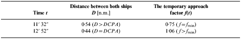
In Figures 3(A) and 3(B) the positions of the own ship and the target ship are presented for the time of reaching f min and the time of reaching DCPA respectively. As might be concluded from Figure 3 and Table 2, the ships reached their f min value (the minimal value of the temporary approach factor f(t) in time t=11′ 32″. Since f min is equal to 0·75, this is a significant domain violation. However, CPA is reached later – in the time t=12′ 52″. For that time f(t) is equal to 1·06, which means that the domain is not penetrated then and might misleadingly suggest that it is not penetrated at all during the whole encounter situation. The example above illustrates the risk that is carried by relying on the DCPA parameter solely, or by limiting oneself to checking only whether the domain would be violated at the closest point of approach.

Figure 3. (A). The own ship (grey icon) and the target ship (black icon) at the moment when f min is being reached: t=11′ 32″. (B). The own ship (grey icon) and the target ship (black icon) at the moment of the closest approach: t=12′ 52″.
Table 2. Different times of reaching fmin and CPA.
3. A NUMERICAL ALGORITHM DETERMINING f min
In the case of some domain models, determining f min analytically may be difficult (domains according to Goodwin and Smierzchalski are good examples). This task, however, may always be solved numerically. In this section a proposed algorithm performing this task is shown. The symbols in the figures have the following meaning:
- (t1,t2)
the time interval considered, for instance – the time when the distance between the own ship and a target object is lesser than a given threshold value,
- a
the distance between the own ship and the most distant point on its domain boundary,
- b
the distance between the own ship and the closest point on its domain boundary,
- δt
a given accuracy of finding the time remaining to reaching f min,
- δf
a given relative accuracy of determining f min value.
a and b are the two extreme values of the distance between own ship and points on its domain boundary. Therefore the distance between own ship and any given point on its domain boundary lies in range (b, a). For any given time t the target object lies on the boundary of the f(t) times enlarged (or shrunk) own ship domain. Thus its distance from the own ship fulfils the condition:
which is illustrated in Figure 4 for the exemplary domains of Coldwell (A) and Goodwin (B). This fact enables us to limit the range of potential values f(t) to:
which largely reduces computational complexity. In Figure 5 (A) a way of finding f(t) for a given moment of time is depicted. Figure 5 (B) presents a process of determining the moment of time, for which f(t) has the minimal value – the value of f min. In both cases the method of bisection of the given range with the given accuracy has been used. The method of bisection (also called binary search) consists of a sequence of iterations. In every iteration the given range of values is divided by two. Then it is checked whether the searched value lies in the left or in the right sub range. Depending on the result, the appropriate sub range is passed on to the next iteration.

Figure 4. (A). Coldwell domain: the distance D(t) between the own ship and the target ship lies within range (b*f(t), a*f(t)). (B). Goodwin domain: the distance D(t) between the own ship and the target ship lies within range (b*f(t), a*f(t)).

Figure 5. (A). Numerical algorithm determining f(t). (B.) Numerical algorithm finding fmin.
Since checking whether a given point lies within a ship domain can be done in constant time, the computational complexity of the proposed solution for any ship domain is:
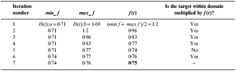
The exemplary sequence of operations performed by the bisection algorithm to find numerically f(t) value for the data from Table 2 (t=11 min and 32 sec) is provided in Table 3. The same sequence of iterations is illustrated in Figure 6, with the iterations 5 and 6 omitted.

Figure 6. Exemplary sequence of iterations for bisection algorithm finding f(t) value with the accuracy δf=0·01.
Table 3. Exemplary sequence of iterations for bisection algorithm finding f(t) with the accuracy δf=0·01.
4. MANOEUVRING TO AVOID DOMAIN VIOLATION
Obviously, knowing the value of the measure (and thus the level of the risk predicted) is one thing and ensuring that the ship’s domain will not be violated is another. While the problem of determining the course alteration necessary for the DCPA value to be safe is solved analytically, there are no analogical formulas for other than circle-shaped domain models. Although there is an abundance of methods for finding safe ship trajectories, they tend to rely heavily on simulation: a trajectory is found first, then it is checked whether the own ship‘s domain will not be penetrated and on this basis the trajectory is either ruled out or passed on for further analysis. Such simulation however is a time-consuming process and therefore many routing and collision avoidance systems choose to rely on the DCPA and TCPA parameters solely. To sum this up – if anything can match the intensity of the development of the ship domain models, it is the consequence with which these models are commonly ignored afterwards. One of the reasons for this is the lack of simple algorithms that would make it possible to take advantage of those more complex domain models. In the following subsection an example of such an algorithm is provided.
4.1. A general algorithm for determining collision avoidance manoeuvre for any given ship domain model
The algorithms in Figure 7 find the minimum necessary course alterations to port (A) and to starboard (B). Again the method of bisection of the given interval with the given accuracy has been used. Both of the algorithms utilize the method from section 3 for finding the f min value for a given course and therefore take all the input parameters listed in section 3. The additional input parameter is:
- δΨ
the accuracy of finding the necessary course alteration.
After determining the two candidate values of the course alteration (for starboard and port respectively), the lesser of them is taken into account. The algorithm is able to find the necessary course alteration within (0, 180) degrees range, but obviously not all values from this range are acceptable. Typically, the course alteration values less then 15 degrees are rounded up to 15 degrees so as to make the manoeuvre ‘readily apparent to another vessel observing visually or by radar’ (COLREGS, Rule 8 b). Also, the course alteration values greater than 60 degrees may not be desired because of economy reasons. In such cases a speed reduction may be applied additionally. The process of finding the necessary speed alteration is analogous to finding the course alteration presented in Figure 7.

Figure 7. Numerical algorithms determining necessary course alteration to port (A) and starboard (B).
4.2. A simulation example: how using the method enforces choosing the manoeuvre in accordance with COLREGS
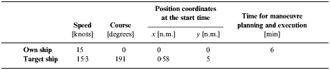
The simulation results for the method described in section 4.1 and utilizing ellipse-shaped domain versus traditional approach (DCPA-based collision avoidance manoeuvre) are presented. First, the simulation parameters are listed in Tables 4 and 5. The domain size given is the same as for Fuji domain presented in section 2.3. However, according to Coldwell the domain centre should be moved from the ship’s position towards the starboard – this modification is used here. The courses of both ships are such that it might be arguable whether this is a crossing or a head-on encounter type.
Table 4. Own ship domain parameters for both methods.
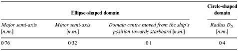
Table 5. Simulation parameters.
The resulting course alterations determined by the proposed method and a DCPA-based method are gathered in Table 6. In the case of the proposed method, the course alteration to starboard is less than that to port. Therefore, a manoeuvre to starboard is performed by the own ship and the conditions of both Rule 14 (Head-on situation) and Rule 15 (Crossing situation) of COLREGS are met:
–a course is altered to starboard (Rule 14 a),
–own ship does not cross ahead of the target ship (Rule 15).
This results in a safe passage of the own ship, no matter whether the target ship considers the situation to be crossing (Figure 8 A) or head-on (Figure 8 B). In case of the traditional approach, the determined course alteration to port is significantly less, which means that in this case the DCPA-based approach favours manoeuvre to port, disregarding Rules 14 and 15. Obviously, no navigator would risk crossing ahead of a target vessel because of a 10 degree course alteration difference between manoeuvres to starboard and port. This however is no excuse for the method, which simply should not encourage an undesirable decision. The potential consequences of such a decision are shown in the Figures 8 C and D. If the target ship identifies the own ship’s manoeuvre to port correctly (and keeps her course), the own ship will safely cross ahead of the target ship (Figure 8 C). However, if the target ship chooses to perform a manoeuvre to starboard (according to Rule 14 a), the two ships might collide (Figure 8 D).
Table 6. Different values of course alteration for the two methods.


Figure 8. (A) The own ship alters her course to starboard and the target ship keeps her course. (B) Both the own ship and the target ship alter their courses to starboard. (C) The own ship alters her course to port and the target ship keeps her course. (D) The own ship alters her course to port and the target ship alters her course to starboard.
5. Applying the measure to the existing formulas
Most of the known formulas for collision risk use the DCPA parameter. An example is equation (19) – a collision risk according to Lisowski [11].
![r \equals \left[ {a_{\setnum{1}} \left( {{{DCPA} \over {D_{S} }}} \right)^{\setnum{2}} \plus a_{\setnum{2}} \left( {{{TCPA} \over {T_{S} }}} \right)^{\setnum{2}} \plus a_{\setnum{3}} \left( {{D \over {D_{S} }}} \right)^{\setnum{2}} } \right]^{ \minus {\setnum{1} \over \setnum{2}}} \comma](https://static.cambridge.org/binary/version/id/urn:cambridge.org:id:binary:20160913095525830-0662:S0373463306003833_eqn19.gif?pub-status=live)
where:
- r
collision risk,
- D
current distance between the own ship and the target ship,
- D S
safe distance of approach (a radius of the circle-shaped domain),
- T S
a time necessary to plan and perform a collision avoidance manoeuvre,
- a1, a2, a3
weight coefficients, dependent on the state of visibility at sea, dynamic length and dynamic beam of the ship and a kind of water region.
In the above equation the DCPA/D S quotient is used, which is exactly the f min value for a circle-shaped domain (section 2.2). In the case of using a different ship domain model, this quotient can be replaced with the f min value obtained for this model, such as the one derived in section 2.2 for the Fuji domain or the one obtained by means of the numerical algorithm presented in section 3. Consequently TCPA might be replaced with the time remaining to reaching f min value and the quotient D/D S with the current value of the temporary approach factor f(t) (section 1). The suggested generalization of the formula, which would hold true for any given ship domain would thus be:
![r \equals \left[ {a_{\setnum{1}} \hskip2 f_{min } \hskip0 ^{\setnum{2}} \plus a_{\setnum{2}} \left( {{T_{f_{min} } } \over {T_{S} }} \right) ^{\hskip-2\setnum{2}} \plus a_{\setnum{3}} \hskip1 \hskip2 f \, \lpar t\rpar ^} \right]^ { \minus {\setnum{1} \over \setnum{2}}}.](https://static.cambridge.org/binary/version/id/urn:cambridge.org:id:binary:20160913095525830-0662:S0373463306003833_eqn20.gif?pub-status=live)
6. SUMMARY AND CONCLUSIONS
In the paper a general concept of a new measure of collision risk has been introduced. It is a versatile meta-measure in the sense that it might be used combined with various ship domain models (including user-defined domains) depending on the particular needs. Detailed formulas derived from the Fuji model of the ship domain have been provided as an example and they might be used directly for collision risk assessment (an example of the already known and useful formula that may benefit from the proposed measure is given in section 5). Additionally, a general algorithm to deal with more complex cases of ship domains has been provided. This algorithm is further used in a simple method of determining the minimal course alteration necessary to avoid a domain violation. Two examples of simulation have also been presented in the paper. Both illustrate the differences between domain-based and DCPA-based approach to risk assessment and collision avoidance. The first one (section 2.3) shows that the ship’s domain may be violated in a time different than that of reaching DCPA. Traditional parameters, DCPA and TCPA, are practically useless in domain violation prediction (in case of domains other than circle-shaped) and thus the method presented is essential for risk assessment. The second example of simulation (section 4.2) focuses on the issue of course alteration manoeuvre. Here the main advantage of the domain-based method is that it favours manoeuvres recommended by COLREGS. The author believes that the measure presented and the collision-avoidance method based on it will help to spread the domain-based approach in collision avoidance systems, since (as the paper shows) this approach is little more complex than the traditional one and naturally encourages navigational decisions in conformity with the legally binding regulations.
ACKNOWLEDGEMENTS
The author would like to thank Prof. A. S. Lenart for his advice and constructive remarks.
