


1. Introduction
Multi-rotor UAVs have a wide range of civilian applications, such as, e.g. environmental studies, rescue and search operations, and weather forecasting (Silano and Iannelli, Reference Silano and Iannelli2016, Reference Silano and Iannelli2020; Quaglia et al., Reference Quaglia, Visconte, Scimmi, Melchiorre, Cavallone and Pastorelli2020). Among these, PA is critical, which refers to technologies enabling more precise and efficient farming, e.g. in growing crops and raising livestock (Daponte et al., Reference Daponte, De Vito, Glielmo, Iannelli, Liuzza, Picariello and Silano2019; AgFunderNews, 2020). The objective of PA is to increase the yield while minimising the required resources. As a result of the rapid global population growth and increased need for food, agricultural production should increase significantly. Sylvester et al. (Reference Sylvester, Rambaldi, Guerin, Wisniewski, Khan, Veale and Xiao2018) found that as the world's population was expected to reach nine billion, agricultural products should increase by $70\%$ by $2050$
 . However, some factors, including global warming, climate change, drought, restricted cropland accessibility and growing demand for freshwater, can jeopardise farming production. In this context, PA has already established a paradigm to increase the quality and productivity of crops and improve working conditions, which can play a key role in developing sustainable agriculture. The degree of acceptance of technologies in farming appears to be high, as also reported by Reinecke and Prinsloo (Reference Reinecke and Prinsloo2017).
Several technologies, methodologies and approaches, including the Global Positioning System (GPS) (Basiri et al., Reference Basiri, Lohan, Moore, Winstanley, Peltola, Hill, Amirian and e Silva2017a), optical and thermal cameras (Basiri, Reference Basiri, Oskoei, Basiri and Shahri2017b; Demkiv et al., Reference Demkiv, Ruffo, Silano, Bednar and Saska2021), Laser Imaging Detection and Ranging (LIDAR) sensors (Bassiri et al.,Reference Bassiri, Asghari Oskoei and Basiri2018), control boards (Silano et al., Reference Silano, Oppido and Iannelli2019), telecommunication (Bonilla Licea et al., Reference Bonilla Licea, Silano, Mounir and Saska2021), and computer science (Silano and Iannelli, Reference Silano and Iannelli2021), need to be applied and embedded in the design of hardware and software architectures to implement and deliver successful PA. The multidisciplinary and multi-sensory nature of multi-rotor UAVs application still stands even for simple tasks, such as UAVs equipped (Tokekar et al., Reference Tokekar, Hook, Mulla and Isler2016), as illustrated in Figure 1.
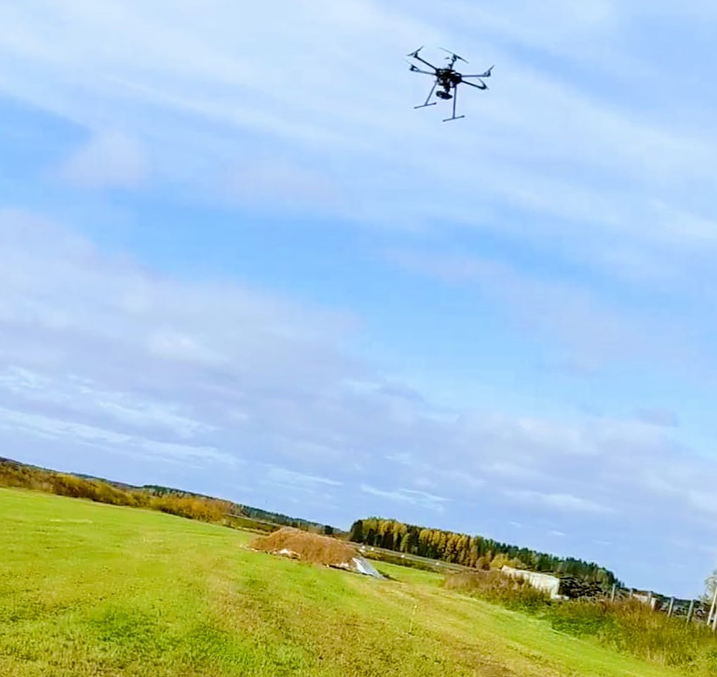
Figure 1. A multi-rotor UAV flying over a farm while collecting information on the soil status
Although motivations and expectations behind PA can be a good driver for its promotion and implementation, there may be several challenges for the agriculture sector. Challenges to address may include energy consumption, safety and collision avoidance (Silano et al., Reference Silano, Baca, Penicka, Liuzza and Saska2021a). In general, multi-rotor UAVs can be used for real-time monitoring or data collection to be fed to suitable decision support systems (Silano et al., Reference Silano, Bednar, Nascimento, Capitan, Saska and Ollero2021b). In addition, they can help with more efficient management of soil, crops and livestock (Stafford, Reference Stafford2000; Radoglou-Grammatikis et al., Reference Radoglou-Grammatikis, Sarigiannidis, Lagkas and Moscholios2020).
Multi-rotor UAVs are characterised by a high-level of manoeuvrability and portability (Silano et al., Reference Silano, Aucone and Iannelli2018). For example, multi-rotor UAVs can go through the shortest path with potentially the maximum roll and pitch angles (they need to tilt to move, Wang et al., Reference Wang, Wang, Ding, Chen and Yang2020; Terlizzi et al., Reference Terlizzi, Silano, Russo, Aatif, Basiri, Mariani, Iannelli and Glielmo2021) and a minimum turning angle (i.e. yaw angle) at a relatively high speed. There are several algorithms that exist for path planning (see Figure 2), each with different capabilities and designed to address specific challenges. However, finding the shortest path for multi-rotor UAVs is a challenging task owing the tight connections between feasibility, safety, energy consumption and computational burden considering the strongly nonlinear dynamics that characterise these devices.
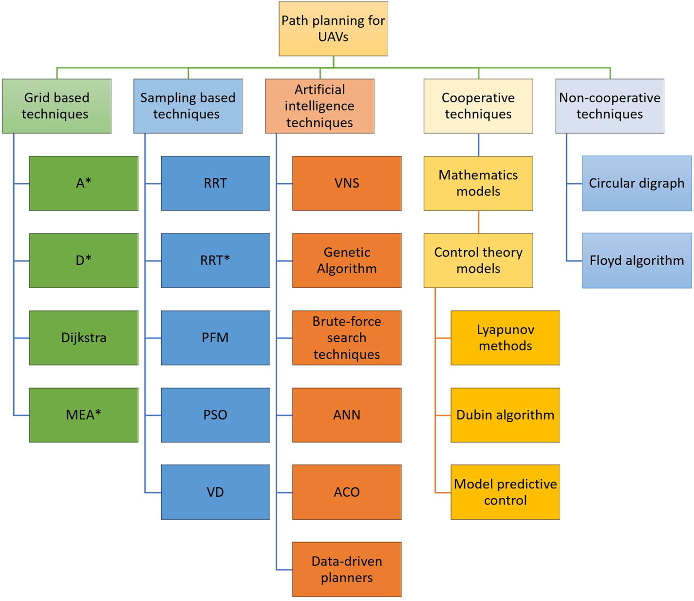
Figure 2. Taxonomy of path-planning techniques
Over the years, several algorithms have been proposed and used to address some aspects of these challenges, especially in the context of PA. For example, Li et al. (Reference Li, Zhao, Zhang and Dong2016) applied a Particle Swarm Optimisation (PSO) algorithm to optimise the flight-time taking into consideration the geometry of the aircraft in three-dimensional (3D) spaces, specifically agricultural environments, while Dewang et al. (Reference Dewang, Mohanty and Kundu2018) used a Genetic Algorithm (GA) to solve path planning to minimise computation time. Similarly, Pham et al. (Reference Pham, Bestaoui and Mammar2017) used GA for solving path-finding problems for aerial robots in PA scenarios while also accounting for the presence of obstacles. Sunny et al. (Reference Sunny, Hossain, Mimma and Hossain2017) and Noguchi et al. (Reference Noguchi, Reid, Benson and Stombaugh1998) attempted to control an Artificial Neural Network (ANN) trained to navigate through semi-structured agricultural environments, with static obstacles in a 3D space. This requires input training data, which may not be available in a new environment. Hao and Yan (Reference Hao and Yan2018) used the Dubins algorithm and the Rapidly Random exploring Tree Star (RRT$^{\star }$ ) algorithm in an obstacle-dense agricultural environment to find the safe path for UAVs and also prioritised obstacle avoidance over other parameters, such as efficiency and performance. Sinha (Reference Sinha2017) designed a path-planning algorithm for an autonomous multi-rotor UAV to tour and cover multiple agricultural regions in the shortest possible time based on Dijkstra's algorithm in two-dimensional (2D) environments. Furthermore, Wang et al. (Reference Wang, Fu, Zhao and Yue2019) and Bakhtiari et al. (Reference Bakhtiari, Navid, Mehri and Bochtis2012) used the Ant Colony Optimisation (ACO) algorithm for obstacle avoidance and optimal path production for agricultural land coverage. Other agricultural machinery (e.g., tractor and combine harvester) equipped with automated steering and navigation systems can benefit from checking the resultant paths. Nolan et al. (Reference Nolan, Paley and Kroeger2017) used a Voronoi Diagram (VD) in 2D spaces for path finding in agricultural area coverage. However, the authors did not seek to find the shortest path. Despite a great deal of effort in this study to address UAV path planning in PA, the research topic still needs further investigation. It is acknowledged that multi-rotor UAVs serve a useful purpose; however, the unwelcome fact is that the use of multi-rotor UAVs has been limited owing to some critical issues, the predominant issue being the limited battery capacity, as presented in Section 3.
This paper discusses motivations, limitations and opportunities of using path-planning algorithms in 3D environments, such as forests and farms. The paper's focus is on path-planning algorithms for 3D environments because the simple customisation of a simple 2D algorithm may not appear to be effective, accurate or reliable (Fu et al., Reference Fu, Chen, Zhou, Zheng, Wei, Dai and Pan2018a). Several approaches and algorithms have attempted to optimise the multi-criteria problem of 3D path finding. It is challenging to optimise energy consumption and minimise flight time and path length while maintaining flight safety and purpose (e.g. solid monitoring). According to the results in Section 3, we suggest a method using the visibility-graph-based $A^{\star }$ algorithm (Noreen et al., Reference Noreen, Khan and Habib2016a, Reference Noreen, Khan, Asghar and Habib2019a; Wang et al., Reference Wang, Liang, Li and Yu2017a, Reference Wang, Liang, Li and Yu2017b) to address path length challenges and time efficiency challenges in agricultural environments. This method is expected to be able to find the optimal path compared to other algorithms (e.g. Haro and Torres, Reference Haro and Torres2006; Roberge et al., Reference Roberge, Tarbouchi and Labonté2012; Yang et al., Reference Yang, Qi, Xiao and Yong2014, Reference Yang, Qi, Song, Xiao, Han and Xia2016b; Baeza et al., Reference Baeza, Ihle and Ortiz2017; Dib et al., Reference Dib, Manier, Moalic and Caminada2017; Fu et al., Reference Fu, Chen, Zhou, Zheng, Wei, Dai and Pan2018a; Korkmaz and Durdu, Reference Korkmaz and Durdu2018; Missura et al., Reference Missura, Lee and Bennewitz2018a, Reference Missura, Lee and Bennewitz2018b; Zammit and Van Kampen, Reference Zammit and Van Kampen2018; Babel, Reference Babel2019; Cabreira et al., Reference Cabreira, Brisolara and Ferreira2019; Noreen et al., Reference Noreen, Khan, Asghar and Habib2019b).
The remainder of this paper is structured as follows. Section 2 characterises path-planning algorithms, Section 3 overviews multi-rotor UAVs path-planning challenges and Section 4 analyses multi-rotor UAVs path-planning methods in agricultural environments. Finally, Section 5 concludes this work.
2. Path-planning algorithms
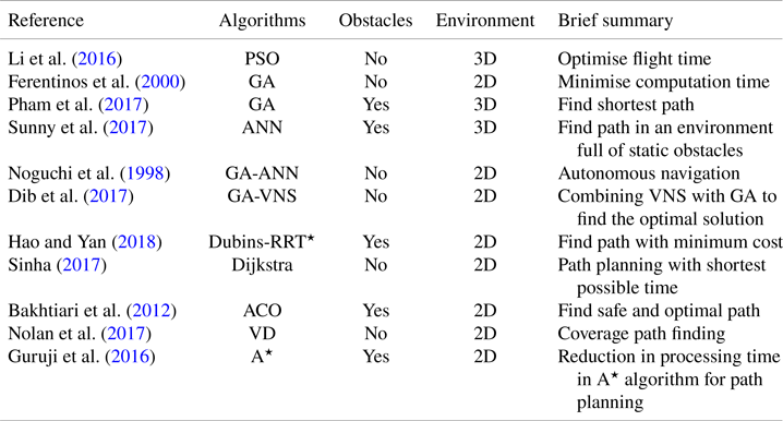
Despite numerous studies on multi-rotor UAV path-planning problems, such as finding the shortest path, least cost routing and maintaining a persistent safe path (e.g., Korkmaz and Durdu, Reference Korkmaz and Durdu2018; Zammit and Van Kampen, Reference Zammit and Van Kampen2018; Babel, Reference Babel2019), open problems about time efficiency and computational burden have required researchers to set up methods and approaches that encompass Artificial Intelligence (AI)-based techniques, cooperative and non-cooperative techniques, network-based techniques and sampling-based techniques. This section aims to collect the most used by describing the bases of their operation and some comparisons of the most important aspects. Figure 2 shows a taxonomy of the most used path-planning techniques, while a brief summary useful to guide the reader during the reading of the survey is reported in Table 1.
Table 1. Summary of path-planning algorithms
2.1 Grid-based techniques
These methods overlay a grid on a configuration space (the space of possible positions that the multi-rotor UAVs may attain) and assume that each configuration is identified with a grid point. The robot can move from one point to an adjacent one as long as this is contained within free space. Such methods support the representation of an environment in memory (see Figure 3), which results in path planning and robot localisation (Yang et al., Reference Yang, Qi, Xiao and Yong2014; Liu et al., Reference Liu, Zhang, Guan and Delahaye2016). There are several grid-based techniques used for path planning, including A star (A$^{\star }$ , Guruji et al. (Reference Guruji, Agarwal and Parsediya2016)), D star (D$^{\star }$
 , Raheem et al. (Reference Raheem2018)) and Dijkstra (Dhulkefl et al., Reference Dhulkefl2019). These techniques uses a heuristic function $f(n)$
 that runs over all nodes $n$
 (i.e. those obtained by partitioning the space), as follows:
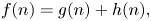
where $g(n)$ is the cost of the path from the start node to goal node and $h(n)$
 represents the estimated cost of the path passing through $n$
 to reach the goal node.
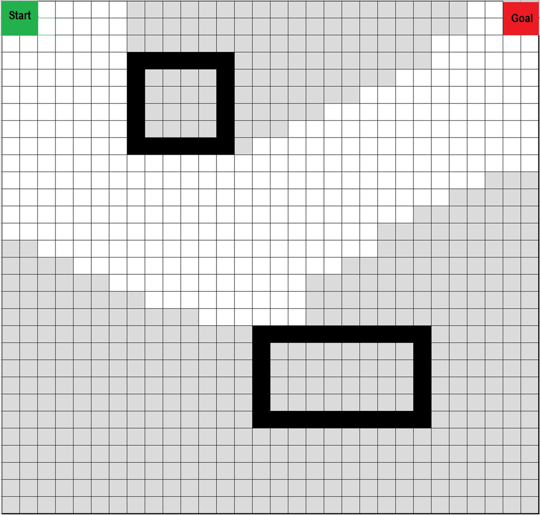
Figure 3. Grid-based method. The green box is the start point, the red box is the target point, the black boxes represent obstacles, the white road contains the grids explored and the grey regions include the grids unexplored
2.1.1 Dijkstra
This algorithm is used to find the shortest distance, or path, from a starting node to a target node in a weighted graph, as shown in Figure 4. It measures the distance value at each node exploring all possible nodes and its optimality depends on the heuristic function used for the NP-hardness of the problem. Examples of use are described, e.g. in Dhulkefl et al. (Reference Dhulkefl2019) and Zhang et al. (Reference Zhang, Wu, Dai and He2021).
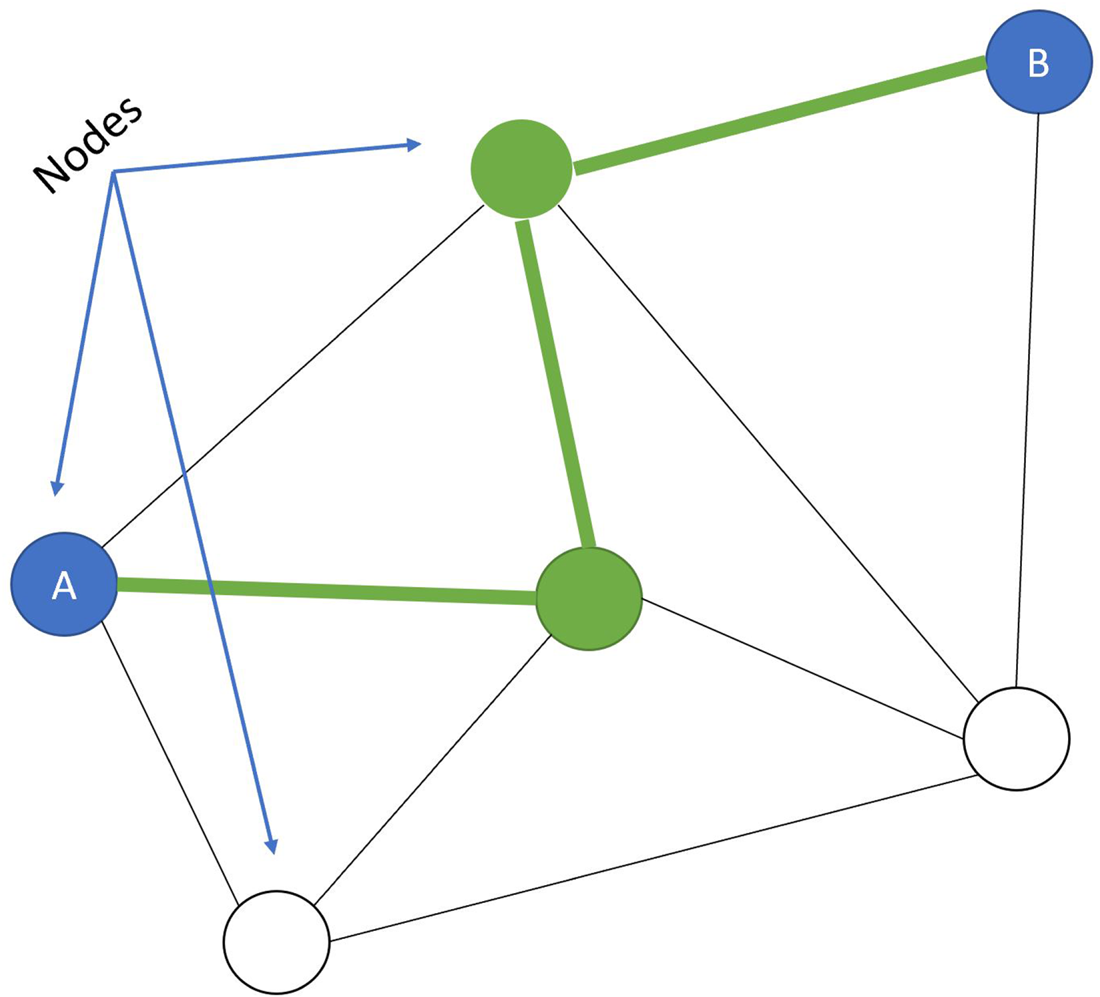
Figure 4. Dijkstra algorithm finds the shortest path (minimum cost) between A and B nodes
2.1.2 A$^{\star }$

This algorithm is almost like Dijkstra, where the only difference is that A$^{\star }$ attempts to look for a better path by using a heuristic function that gives priority to nodes that are supposed to be better than others. In other words, while Dijkstra explores all possible node combinations, A$^{\star }$
 explores the graph using only the paths made where the next node is superior to the others. The A$^{\star }$
 algorithm does this by maintaining a tree of paths originating at the start node and extending those paths one edge at a time until its termination criterion is satisfied (Guruji et al., Reference Guruji, Agarwal and Parsediya2016; Fu et al., Reference Fu, Chen, Zhou, Zheng, Wei, Dai and Pan2018a; Korkmaz and Durdu, Reference Korkmaz and Durdu2018).
2.1.3 D$^{\star }$

The D$^{\star }$ algorithm can be thought of as a dynamic A$^{\star }$
 because it is based on a graph-based real-time short path with cost updating or changing. In D$^{\star }$
 , when the initial path is blocked, an incremental search algorithm can take advantage of previous calculations. Such an incremental approach is often used in robotics, e.g. Raheem et al. (Reference Raheem2018) used the D$^{\star }$
 algorithm for path planning in a dynamic environment.
2.2 Sampling-based techniques
Sampling-based algorithms represent the configuration space with a roadmap of sampled configurations. A basic algorithm samples configurations in space and retains those in free space to use as milestones to find a path that connects start and goal (see Figure 5). These algorithms are more suitable in 3D spaces (LaValle, Reference LaValle2006), examples include PSO, the Potential Field (PF) method, Probabilistic Roadmaps (PRs), the Rapidly exploring Random Tree (RRT), RRT$^{\star }$ and VD (Elbanhawi and Simic, Reference Elbanhawi and Simic2014; do Ó et al., Reference do Ó, Alexandre Prates, Mendonça, Lourenço, Marques and Barata2019).
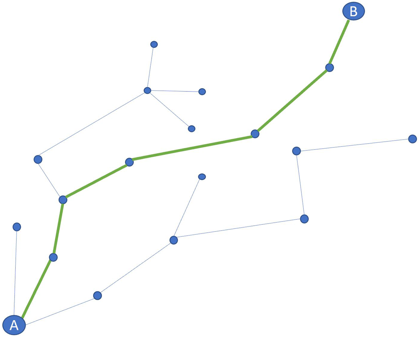
Figure 5. The sampling algorithm makes a tree to find the path between A and B
2.2.1 RRT
The algorithm is designed to efficiently search non-convex, high-dimensional spaces by randomly building a tree. The tree is constructed incrementally from samples drawn randomly from the search space and is inherently biased to grow towards large unsearched areas of the problem (Kuffner and LaValle, Reference Kuffner and LaValle2000; Yang et al., Reference Yang, Qi, Xiao and Yong2014). It is made of samples that randomly appear in the search. The main advantage of the algorithm is the wide application spectrum in robot motion planning and strength in multiple UAV collision avoidance (Kuffner and LaValle, Reference Kuffner and LaValle2000; Hoang, Reference Hoang2019).
2.2.2 RRT$^{\star }$

This is an optimised version of RRT. When the number of nodes approaches infinity, this algorithm will deliver the shortest possible path to the goal. The basic principle of RRT$^{\star }$ is the same as that of RRT. Noreen et al. (Reference Noreen2016b) used RRT$^{\star }$
 to find the shortest path and the smoothest path between the initial position and the target.
2.2.3 Potential field method
The concept of electrical charges inspired the PF method. If we see our robot as an electrically charged particle, then obstacles should have the same type of electrical charge to repel the robot from them self. This idea is illustrated in Figure 6. In the same context, Yingkun (Reference Yingkun2018), Aggarwal and Kumar (Reference Aggarwal and Kumar2020) and Budiyanto et al. (Reference Budiyanto, Cahyadi, Adji and Wahyunggoro2015) used the PF method algorithm for UAVs path planning in agricultural environments.
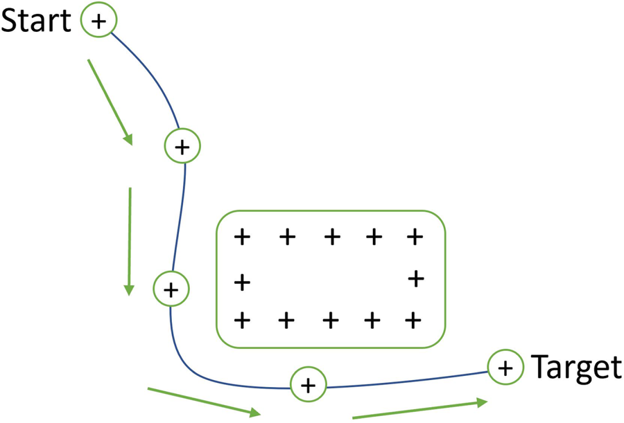
Figure 6. Potential field method
2.2.4 Particle swarm optimisation
This technique is a computational approach to address the challenge of optimisation. PSO can solve the problem by estimating multiple candidate solutions and travelling through the search space. This is based on a mathematical model that uses the position and velocity of particles. Li et al. (Reference Li, Zhao, Zhang and Dong2016) and Ou et al. (Reference Ou, Liu and Zhao2017) employed this algorithm to optimise flight paths for UAVs used in agriculture.
2.2.5 Voronoi diagram
This method is employed to divide road maps into areas based on the distance to waypoints. In building road maps, each method performs differently regarding the nodes and edges. The VD describes nodes near all points around obstacles, as shown in Figure 7. The path generated as a graph from the VD is highly safe because the obstacles are so far from all the path edges (Aggarwal and Kumar, Reference Aggarwal and Kumar2020). Nolan et al. (Reference Nolan, Paley and Kroeger2017) used this algorithm for path optimisation in an agricultural environment.
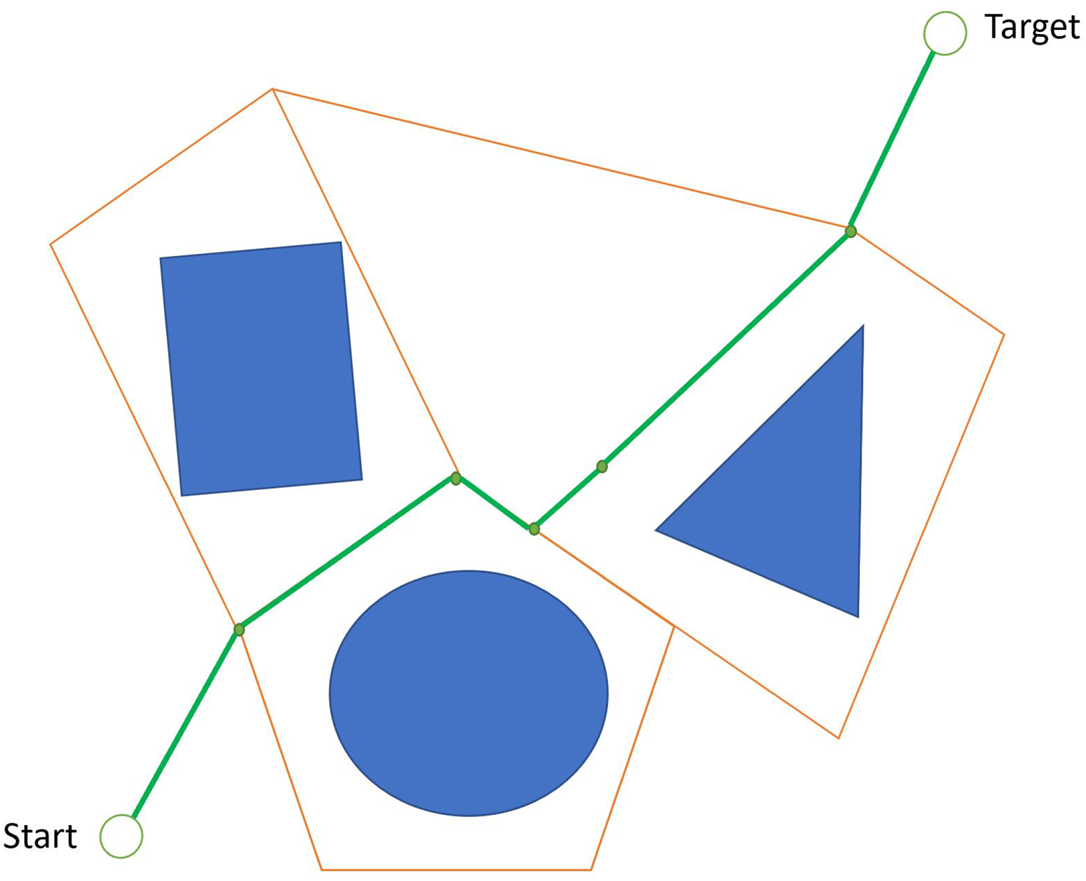
Figure 7. The Voronoi diagram
2.3 AI-based techniques
These techniques think intelligently in the same way an intelligent human would. One of the key aspects of AI is efficient Computational Intelligence (CI) algorithms (Zhao et al., Reference Zhao, Zheng and Liu2018), such as neural networks and evolutionary algorithms. There are several AI-based methods for multi-rotor UAVs path planning, including ACO (Deb, Reference Deb2011), ANN (ANN, Reference Liang and Wang2020), brute force search (Brassai et al., Reference Brassai, Iantovics and Enăchescu2012), GA (Pham et al., Reference Pham, Bestaoui and Mammar2017), heuristic search (Zhao et al., Reference Zhao, Zheng and Liu2018), Variable Neighbourhood Search (VNS) (Hansen et al., Reference Hansen, Mladenović and Pérez2010) and data-driven planners (Tamar et al., Reference Tamar, Wu, Thomas, Levine and Abbeel2016).
2.3.1 Ant colony optimisation
This is a class of optimisation algorithms based on the ability of ants to find the shortest path to the food source. Ants repeatedly jump to eventually acquire their food. Ants record their positions and the quality of their solutions so that in later iterations, more ants locate better solutions. Such an approach can also be used for multi-rotor UAVs path planning (Deb, Reference Deb2011). Yang et al. (Reference Yang, Wang, Li, Yang, Luo, Zhang, Zhang and Chen2016a) developed an ACO algorithm to shape a multi-rotor UAVs path in a cluster. The results indicated that this strategy is more efficient than traditional algorithms.
2.3.2 Artificial neural network
These algorithms are based on the human nervous system and are applied for solving different nonlinear problems that require foreknowledge. Taking advantage of the limitations of experimental models with limited supervision can help solve the parameter recovery problem. ANN can also be employed for multi-rotor UAVs path planning. For instance, Eski and Kuş (Reference Eski and Kuxş2019) exploited an ANN-based Proportional-Integral-Derivative (PID) controller (Tang et al., Reference Tang, Wang, Gu and Gu2020) to handle multi-rotor UAVs, which yielded favourable results.
2.3.3 Brute force search technique
This technique is a typical problem-solving method and an algorithmic paradigm systematically enumerating all possible candidates to solve and check if they satisfy the problem statement. Sinha (Reference Sinha2017) employed this technique to determine the closest entry or exit node of multi-rotor UAVs path planning in agriculture.
2.3.4 Genetic algorithm
This is used to establish the best possible solutions to search and optimise problems tapping into bio-inspired operators, such as crossover, mutation and selection. Pham et al. (Reference Pham, Bestaoui and Mammar2017) used GA for path planning to diminish the path length of an airborne robot in an agricultural environment with concave obstacles. Similarly, Hayat et al. (Reference Hayat, Yanmaz, Brown and Bettstetter2017) used GA to boost the working path and the performance of multi-rotor UAVs.
2.3.5 Heuristic search techniques
They are used for optimal multi-rotor UAVs path planning from the source to the destination point via the cost estimation method. The technique can solve a problem quicker than classic methods (Ferentinos et al., Reference Ferentinos, Arvanitis, Kyriakopoulos and Sigrimis2000). This is a shortcut because we often trade accuracy, completeness, optimality or precision for speed. A heuristic (or a heuristic function) observes search algorithms, evaluates the available information at each branching step and decides on which branch to follow by ranking alternatives. Ferentinos et al. (Reference Ferentinos, Arvanitis, Kyriakopoulos and Sigrimis2000) examined two exploratory optimisation methods using motion planning for autonomous agricultural vehicles. This comparison showed that the Simulated Annealing (SA) algorithm outperformed GA.
2.3.6 Variable neighbourhood search
This algorithm, suggested by Hansen et al. (Reference Hansen, Mladenović and Pérez2010), is a metaheuristic approach to overcome a set of combinatorial and global optimisation problems. These neighbourhoods study the current solution and move on to new ones only if an improvement was made. The local search method is applied repeatedly to get from solutions in the neighbourhood to local optimisation. Hidalgo-Paniagua et al. (Reference Hidalgo-Paniagua, Vega-Rodríguez and Ferruz2016) used variable neighbourhood paths and produced proper ones with shorter lengths, greater safety and softer movements to solve the path-planning problem.
2.3.7 Data-driven planners
Much work has been done on data-driven planners (e.g. Tamar et al., Reference Tamar, Wu, Thomas, Levine and Abbeel2016; Xiao et al., Reference Xiao, Wan, Zhuo, Lin and Liu2019), but little has focused on how search-based planners can benefit from data-driven ones. For data-driven search-based planners, significant challenges include the discrete nature of their path search procedures, which make it complicated to employ learning via back propagation. As a solution, Vlastelica et al. (Reference Vlastelica, Paulus, Musil, Martius and Rolínek2019) treated a search algorithm as a black-box function. Through black-box optimisation, it learnt visual representations of obstacles. Although this approach can recognise obstacles in raw image inputs, it can still improve the search efficiency because internal search steps are black-boxed. As another relevant attempt, Bhardwaj et al. (Reference Bhardwaj, Choudhury and Scherer2017) proposed a data-driven best first-search method that learnt a heuristic function to forecast the exact cost from every node to the goal. While this application can make the search systemic, interpreting per node is expensive, cumbersome and, in many cases, not expandable, especially when only raw image inputs are available.
2.4 Cooperative techniques
By combining control theory models, nature-inspired models, machine-learning models and mathematical models help to understand and analyse most learning methods and classify them into different categories, such as problem-solving and graphic organisers for multi-rotor UAVs path planning (Aggarwal and Kumar, Reference Aggarwal and Kumar2020).
2.4.1 Mathematical models
Mathematical functions and equations, such as the Bézier curve and Lyapunov function (Mueller et al., Reference Mueller, Hehn and D'Andrea2015), can be used to solve multi-rotor UAVs path-planning problems.
2.4.2 Dubins algorithm
Dubins paths help find the shortest possible path for multi-rotor UAVs models based on algebraic solutions. These paths include three sections based on arcs or straight lines of a specified radius. The Dubins algorithm can be used for multi-rotor UAVs path planning. Lugo-Cárdenas et al. (Reference Lugo-Cárdenas, Flores, Salazar and Lozano2014) employed this algorithm to track the trajectory generator and the trajectory tracking strategy used to search and find a path.
2.5 Non-cooperative techniques
Here, planning algorithms and techniques operate autonomously and are aware of one another's algorithms, including graph search algorithms, such as a Floyd algorithm used for multi-rotor UAVs path planning (Aggarwal and Kumar, Reference Aggarwal and Kumar2020).
2.5.1 Floyd algorithm
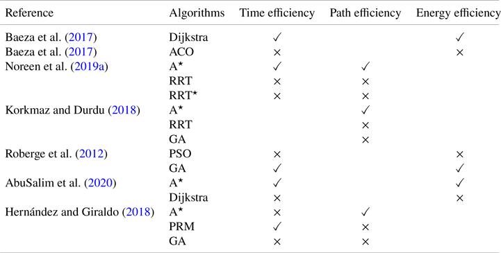
It is employed in multi-rotor UAVs path planning to find the shortest possible paths in a negative or positive edge-weighted graph (Cormen et al., Reference Cormen, Leiserson, Rivest and Stein2009). Yang et al. (Reference Yang, Xi, Wang and Xie2018) proposed cooperative patrol path planning for multi-rotor UAVs and applied the Floyd–Warshall algorithm to predict and optimise the starting path (Table 2).
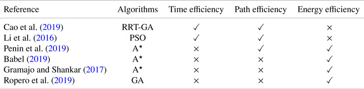
Table 2. Relative comparison of the existing proposals in path-planning algorithms (Time efficiency, Path efficiency, Energy efficiency): $\checkmark$ , considered; $\times$
 , not considered
3. Path-planning challenges
These challenges are interesting in various aspects, such as complexity, power and multi-rotor UAVs optimisation. This section seeks to discover path-planning challenges in agricultural scenarios with multi-rotor UAVs. Path-planning methods mainly aim at reducing costs and running time for optimal path planning. They should optimise energy and minimise the risk of an accident between fleet of multi-rotor UAVs (Lozano-Pérez and Wesley, Reference Lozano-Pérez and Wesley1979; Bortoff, Reference Bortoff2000; Yang and Kapila, Reference Yang and Kapila2002). We will explore four path planning problems: path length (see Section 3.1), time efficiency (see Section 3.2), collision avoidance (see Section 3.3) and energy efficiency (see Section 3.4).
3.1 Path length
This challenge is indeed the distance between the start and endpoints of a target. Zhao et al. (Reference Zhao, Zheng and Liu2018) published a review of $231$ articles in major journals and conference proceedings over the past decade, which provides a comprehensive analysis of AI-based multi-rotor UAVs path-planning literature. They compared and evaluated a diverse group of AI algorithms in multi-rotor UAVs path planning, different features in different types, time domains, and environmental modelling methods in different space domains. In Cekmez et al. (Reference Cekmez, Ozsiginan and Sahingoz2017) and Shao et al. (Reference Shao, Peng, He and Du2020), a new algorithm was proposed to find an optimal path. Cao et al. (Reference Cao, Zou, Jia, Chen and Zeng2019) improved the RRT algorithm and combined it with GA to minimise the distance between the start and endpoints (in 0$\cdot$
 47 s $100\%$
 success rate). Hafez et al. (Reference Hafez, Kamel, Jardin and Givigi2017) suggested that the hierarchical fuzzy logic controller algorithm could overcome computational sophistication in assigning multiple missions by taking advantage of its two sets of fuzzy logic controllers. In Table 3, we analyse the performance of these algorithms in 3D environments.
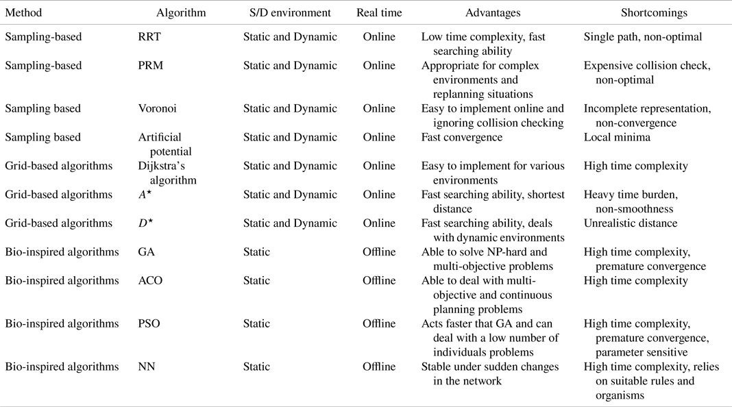
Table 3. An analysis of path-planning algorithms with respect to the environment, the advantages, the shortcomings and the method
3.2 Time efficiency
Multi-rotor UAVs manage target operations from the start to the end point with obstacles in the shortest possible time. For example, Li et al. (Reference Li, Zhao, Zhang and Dong2016) used the PSO algorithm to produce an optimal trajectory for each team after verifying the optimal time. Nonetheless, they did not consider the inappropriateness of the proposed algorithm for a single multi-rotor UAV in large environments and long paths.
To cope with the task in the shortest possible time and gather enough measurements to reach the target with a certain level of confidence, Penin et al. (Reference Penin, Giordano and Chaumette2019) showed a robust perception-aware bi-directional A$^{\star }$ planner for differentially flat systems, which was used for a unicycle and a multi-rotor UAV. He applied a derivative-free Kalman filter to approximate the belief dynamics in the flat space. Babel (Reference Babel2019) pursued the issue of flight planning, where aircraft should reach their destination, and found the shortest path using the A$^{\star }$
 algorithm in the shortest possible time. This paper received some criticism because an increased number of multi-rotor UAVs made the path-planning problem even more difficult. The maximum path length deviation was less than or equal to $0{\cdot }1\%$
 with no more than four multi-rotor UAVs, while it was less than $2\%$
 with six aircraft. Hence, the algorithm offers different results, and thus, is not implemented in a real environment.
3.3 Collision avoidance
This challenge consists of multi-rotor UAVs that have to detect the trajectory of another multi-rotor UAV to prevent physical damage. For instance, Huang et al. (Reference Huang, Teo and Tan2019) provided a general study for researchers to deal with multiple UAVs collisions. The existing literature on this technique is classified based on the algorithm. For example, Dewangan et al. (Reference Dewangan, Shukla and Godfrey2019) used a Grey Wolf Optimiser (GWO) algorithm for multi-rotor UAVs path planning. Although the results yielded a low path calculation cost, they did not fully consider the GWO algorithm. Therefore, GWO failed to present a globally optimal solution. The search technique used in basic GWO is based fundamentally on the random walk.
In a similar vein, Primatesta et al. (Reference Primatesta, Guglieri and Rizzo2019) proposed a novel technique using the A$^{\star }$ algorithm to determine a useful path that minimised the collision risk of a multi-rotor UAV with multiple targets, while considering the risk map as discretised in a 2D space, i.e. a fixed and constant altitude of flight. However, they did not consider the map in a 3D space, different altitudes, and also, Qie et al. (Reference Qie, Shi, Shen, Xu, Li and Wang2019) solved a multi-rotor UAV target and flying multi-rotor UAVs problems using a multi-agent deep deterministic policy gradient algorithm. They claimed that the proposed method could use and demonstrate decision-making data from deep reinforcement learning to encounter dynamic environments effectively. However, they did not compare it with other algorithms to determine its effectiveness. Likewise, Yang et al. (Reference Yang, Zhang, Zhang and Xiangmin2019) considered time variables and improved mechanisms for standard PSO, referred to as the spatially refined voting mechanism.
3.4 Energy efficiency
This challenge is considered as a path-planning problem that achieves the lowest energy consumption by multi-rotor UAVs. Fu et al. (Reference Fu, Yu, Xie, Chen and Mao2018b) proposed an exploratory evolutionary algorithm, examined factors influencing the multi-rotor UAVs flight trajectory and suggested three cost functions. Gramajo and Shankar (Reference Gramajo and Shankar2017) provided a multi-rotor UAVs path-planning algorithm that defined rotation rates optimised by vehicle manoeuvrability based on an exploration algorithm and a modified version of A$^{\star }$ . Ropero et al. (Reference Ropero, Muñoz and R-Moreno2019) used GA to solve the travelling salesman problem for Unmanned Ground Vehicles (UGVs). Although they implemented a search algorithm for multi-rotor UAVs based on the A$^{\star }$
 algorithm, they did not consider any inherent physical limitations for land and air vehicles, including land slope, wind speed or atmospheric density. Instead, they proposed a specific scenario that would address the problem of limited energy multi-rotor UAVs and UGV charging stations.
4. Multi-rotor UAVs path-planning algorithm problems in precise agriculture
This section deals with presenting multi-rotor UAVs path-planning algorithms in the context of precision agriculture. The taxonomy is divided into three parts: the grid-based algorithms (see Section 4.1, which lists the most important grid-based algorithms, their advantages and drawbacks); the sampling-based techniques (see Section 4.2, which explains the advantages of having a map in the path planner design); and finally the visibility-graph-based algorithms (see Section 4.3, which includes their importance for navigation purposes).
4.1 Grid-based algorithms
Regarding agricultural multi-rotor UAVs navigation, we should consider the path-planning algorithm in 3D environments. Grid-based algorithms similar to Dijkstra, D$^{\star }$ and A$^{\star }$
 in 3D environments (Tan et al., Reference Tan, Zhao, Wang, Zhang and Li2016) are quite different from the algorithm in 2D environments owing to the increasing node for every single movement. It should be noted that 2D environments only allow for horizontal movements in four basic moving styles, which include moving forward, backward, left and right. However, the number of horizontal and vertical moving styles in 3D environments is increased from eight to $26$
 . The increasing number of nodes in 3D environments creates more alternatives for moving steps. However, they also change the time process and memory cost of the algorithm, as shown in Figure 8. For example, the A$^{\star }$
 algorithm maintains an open and a closed list (Fu et al., Reference Fu, Chen, Zhou, Zheng, Wei, Dai and Pan2018a). The former contains unexplored nodes in three dimensions, while the latter contains units chosen or rejected to be placed on the resulting path. The increasing movement choice will directly affect the size of the open list. The same problem arises with the time spent on the process. The computational time for path generation exhibits a direct relationship with the number of nodes as A$^{\star }$
 requires more time to process the nodes. Agricultural environments, such as farms, are large. The grid-based algorithm requires the computation of each node, and thus, it takes more time to process the nodes (Baek and Choi, Reference Baek and Choi2017; Hao and Yan, Reference Hao and Yan2018; Korkmaz and Durdu, Reference Korkmaz and Durdu2018; Missura et al., Reference Missura, Lee and Bennewitz2018b). These algorithms may work in a familiar environment, yet they may not provide inseparability in complex environments.
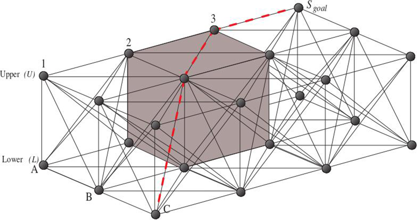
Figure 8. Grid-based method in a 3D environment (Nash et al., Reference Nash, Koenig and Tovey2010)
4.2 Sampling-based techniques
These techniques require pre-determined information about workspace configuration according to the 3D environments. In this case, cell decomposition and roadmap techniques are two of the significant sampling-based techniques.
Cell decomposition is the path configuration between the initial point and the target. The configuration can be determined by dividing the free space of a robot into smaller areas known as cells, each shown as a node in this diagram. As shown in Figure 9, Exact Cell Decomposition (ECD) finds its way. Approximate Cell Decomposition (ACD) is less concerned but can have the same result as ECD. A roadmap consists of two sections: construction and quarry. The construction section calculates the connection of the free space by determining network curves in a 3D environment. After roadmap construction, the first and last configuration points are overcome in the quarry section (Aggarwal and Kumar, Reference Aggarwal and Kumar2020). This method is used by algorithms, such as RRT, RRT$^{\star }$ , PR, PSO and VD. Sampling-based methods, such as RRT, PR and their improved versions, can quickly produce an almost globally optimal solution. Many RRT algorithms have a poor rate of convergence at high-dimensional bandwidth locations. They often prioritise speed over optimality. RRT$^{\star }$
 has a higher convergence rate than RRT and finds an almost optimal path through subsequent processing. However, limitations like high memory usage, poor convergence rate and space exploration render 3D environments inappropriate for the complex problems in Majeed and Lee (Reference Majeed and Lee2018) by discarding beneficial samples.
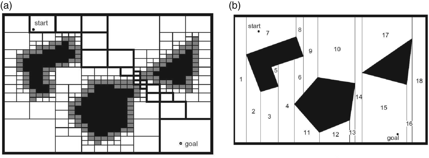
Figure 9. (a) Exact cell decomposition; (b) adaptive cell decomposition (Aggarwal and Kumar, Reference Aggarwal and Kumar2020)
Regardless of their technical similarity, sampling-based and grid-based techniques employ different node-selection strategies. Hence, problems with node-based methods persist in 3D environments, particularly in agriculture. Additionally, sampling-based techniques find longer paths than grid-based techniques. In this context, another method can be used to overcome these agricultural multi-rotor UAV path-planning problems, called the visibility-graph-based method.
4.3 Visibility-graph-based algorithms
Visibility-graph-based algorithms implemented in 3D environments (Scholer et al., Reference Scholer, la Cour-Harbo and Bisgaard2011) have been developed from computer science. In agricultural environments, like farms, nodes and links do not appear naturally. Hong and Murray (Reference Hong and Murray2016) and Wooden (Reference Wooden2006) studied open area path-finding approaches, such as the visibility graph. Huang and Teo (Reference Huang and Teo2019) and Yang et al. (Reference Yang, Qi, Song, Xiao, Han and Xia2016b) compared the optimality of the path in real-time with 3D complex static and dynamic environments, such as greenhouses. Yang et al. (Reference Yang, Qi, Song, Xiao, Han and Xia2016b) were particularly successful in robotic applications. Also, Basiri (Reference Basiri2020) used a visibility graph in areas with no urban paths, such as parks.
The visibility graph is a graph whose edges are augmented in each pair of mutually visible vertices. The visibility-graph-based method is employed for various purposes, including navigation of multiple robots in 3D environments. It is the best method for path planning in outdoor and 3D agricultural environments to calculate the path between nodes. As reported in Table 4, A$^{\star }$ performs better than other algorithms, and regarding features, the visibility graph is without structure environments, like in farms and parks. It can be claimed that using an A$^{\star }$
 algorithm based on the visibility graph will be very efficient to find the path in agricultural environments. Figure 10 outlines the visibility-graph-based method described by Wooden (Reference Wooden2006) and Majeed and Lee (Reference Majeed and Lee2018).
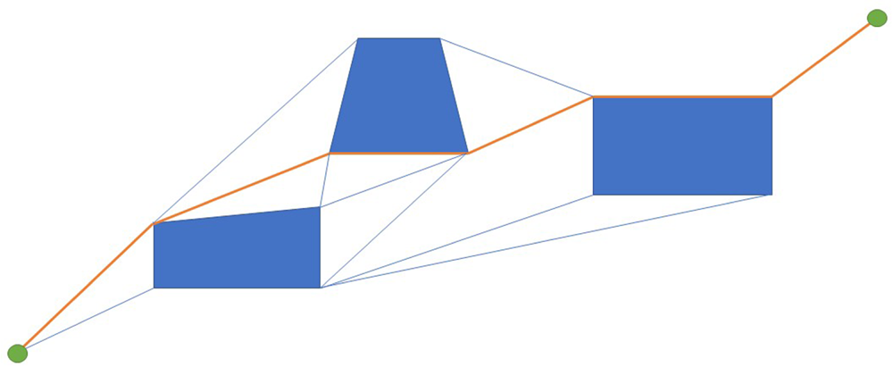
Figure 10. Visibility-graph-based method
Table 4. Comparison of performance results of algorithms (Time efficiency, Path efficiency, Energy efficiency): $\checkmark$ , better; $\times$
 , worse; free space, not considered
5. Conclusions
This paper explores and analyses different approaches to solve multi-rotor UAVs path-planning problems and discusses various multi-rotor UAVs path-planning methods in 3D spaces, like agricultural environments. Also, a visibility-graph-based method is suggested using the A$^{\star }$ algorithm to address the path length, time efficiency and energy efficiency challenges and it has the ability to best fit agricultural environments.
Supplementary material
The supplementary material for this paper can be found at https://doi.org/10.1017/S0373463321000825.
Acknowledgments
This work was partially funded by the ECSEL Joint Undertaking (JU) research and innovation programme COMP4DRONES under grant agreement no. 826610 and by the European Union's Horizon 2020 research and innovation programme AERIAL-CORE under grant agreement no. 871479. The JU receives support from the European Union's Horizon 2020 research and innovation programme and Spain, Germany, Austria, Portugal, Sweden, Finland, Czech Republic, Poland, Italy, Latvia, Greece and Norway.


