2.1. Quaternion

A quaternion is an extension of the complex number to R⁴. A quaternion is defined by ${\bi q}\equiv [\varrho^{T}\ q_{4}]^{T}$, where $\varrho \equiv [q_{1}\ q_{2}\ q_{3}]^{T}$ is a Three-Dimensional (3D) vector (called the vector part), and q ₄ is a scalar (called the scalar part). The basic operations of quaternions are given as follows:

(1)$$\eqalign{{\bi q}^{\prime}+{\bi q}&=[\matrix{\varrho^{\prime T} +\varrho^T & q_4^{\prime} + q_4}]^T \cr \lambda {\bi q}&=[\matrix{\lambda \varrho ^T & \lambda q_4}]^T \cr {\bi q}^{\prime}\otimes {\bi q}&\equiv \left[\matrix{ q_4^{\prime} \varrho +q_4 \varrho^{\prime}-\varrho^{\prime}\times \varrho \cr q_4^{\prime} q_4 -\varrho^{\prime}\cdot \varrho }\right]}$$

The norm of the quaternion is defined as $\Vert {\bi q} \Vert=\sqrt{{\bi q}\otimes {\bi q}}^{\ast} =\sqrt{{\bi q}^{T}{\bi q}}$, where ${\bi q}^{\ast} =[-\varrho^{T} q_{4}]^{T}$ is the conjugate of quaternion q. If $\Vert{\bi q}\Vert = 1, {\bi q}$ is called the unit quaternion, which is usually used to describe the rotation of a rigid body. Successive rotations can be accomplished by using unit quaternion multiplication. As seen in Equation (1), quaternion multiplication in this paper is defined using the convention of Lefferts et al. (Reference Lefferts, Markley and Shuster1982), in which the quaternion multiplication expression appears in the same order as the corresponding attitude matrix multiplication. Because the definition of quaternion multiplication is different from that in Wu et al. (Reference Wu, Hu, Hu, Li and Lian2005), the following formula derivations have some differences to those in Wu et al. (Reference Wu, Hu, Hu, Li and Lian2005) in form; however, they are the same in nature.

For a fixed 3D vector r, the expression in the different frames can be related by

(2)$${\bi r}^N={\bi q}\otimes {\bi r}^O\otimes {\bi q}^{\ast}$$

where q is the unit quaternion from the O frame to the N frame and ${\bi r}^{O}$ and ${\bi r}^{N}$ are the same vector r expressed in the O frame and N frame, respectively. It is noted here that a vector is treated equivalently to its corresponding quaternion with a vanishing scalar part when computing expressions similar to Equation (2). The attitude matrix is related to the unit quaternion by

(3)$${\bi A}({\bi q})=\lpar q_4^2-\Vert \varrho \Vert^2 \rpar {\bi I}_{3\times 3} +2\varrho \varrho^{\rm T} - 2q_4 [\varrho \times]$$

2.2. Dual number

A dual number is defined as (Clifford, Reference Clifford1873)

(4)$$\mathop{a}\limits^{\frown} = a + \varepsilon a^{\prime}$$

where a and a′ are real numbers, called the real part and dual part, respectively; ε is a dual unit satisfying $\varepsilon^{2}=0$ and $\varepsilon \neq 0$. By definition, the basic operations of dual numbers are given as follows:

(5)$$\eqalign{{\mathop{a}\limits^{\frown}}_1 + {\mathop{a}\limits^{\frown}}_2 &=(a_1 +a_2)+\varepsilon (a_1^{\prime} +a_2^{\prime}) \cr \lambda \mathop{a}\limits^{\frown} &=\lambda a+\varepsilon \lambda {a}^{\prime},\quad \forall \lambda \in {\open R} \cr {\mathop{a}\limits^{\frown}}_1 {\mathop{a}\limits^{\frown}}_2 &=a_1 a_2 +\varepsilon (a_1 a_2^{\prime} +a_2 a_1^{\prime})}$$

A dual vector is a generalisation of a dual number whose real and dual parts are both 3D vectors. Given two dual vectors ${\mathop{\bi v}\limits^{\frown}}_{1} ={\bi v}_{1} +\varepsilon {\bi v}_{1}^{\prime}$ and ${\mathop{\bi v}\limits^{\frown}}_{2} ={\bi v}_{2} +\varepsilon {\bi v}_{2}^{\prime}$, the dot product and cross product are defined as follows:

(6)$$\eqalign{{\mathop{\bi v}\limits^{\frown}}_1 \cdot {\mathop{\bi v}\limits^{\frown}}_2 ={\bi v}_1 \cdot {\bi v}_2 +\varepsilon ({\bi v}_1 \cdot {\bi v}_2^{\prime} +{\bi v}_1^{\prime} \cdot {\bi v}_2) \cr {\mathop{\bi v}\limits^{\frown}}_1 \times {\mathop{\bi v}\limits^{\frown}}_2 ={\bi v}_1 \times {\bi v}_2 +\varepsilon ({\bi v}_1 \times {\bi v}_2^{\prime} +{\bi v}_1^{\prime} \times {\bi v}_2)}$$

As stated in Wu et al. (Reference Wu, Hu, Hu, Li and Lian2005), a unit dual vector is known as the Plücker coordinate or the Plücker line, which is usually used to represent a line in 3D space. The real part is the unit direction vector of a line, and the dual part is the line moment with respect to the origin of the coordinate frame. As seen in Figure 1, a Plücker line $\mathop{\bi L}\limits^{\frown} ={\bi l}+\varepsilon {\bi m}$ that passes through the point p/ is defined using two 3D vectors l and m where ${\bf m} = {\bi p} \times {\bi l}$.

Figure 1. Plücker line and frame rotation.

2.3. Dual Quaternion

A dual quaternion is a quaternion with dual number components, or in other words, it can also be regarded as a dual number with quaternion components. Thus, a dual quaternion is defined as

(7)$$\mathop{\bi q}\limits^{\frown} = {\bi q}+\varepsilon {\bi q}^{\prime}$$

where q and ${\bi q}^{\prime}$ are both quaternions. The basic operations of dual quaternions are given as follows:

(8)$$\eqalign{{\mathop{\bi q}\limits^{\frown}}_1 + {\mathop{\bi q}\limits^{\frown}}_2 &=({\bi q}_1 +{\bi q}_2)+\varepsilon ({\bi q}_1^{\prime} +{\bi q}_2^{\prime}) \cr \lambda \mathop{\bi q}\limits^{\frown} &=\lambda {\bi q} + \varepsilon \lambda {\bi q}^{\prime},\quad \forall \lambda \in {\open R} \cr {\mathop{\bi q}\limits^{\frown}}_1 \otimes {\mathop{\bi q}\limits^{\frown}}_2 &={\bi q}_1 \otimes {\bi q}_2 +\varepsilon ({\bi q}_1 \otimes {\bi q}_2^{\prime} +{\bi q}_1^{\prime} \otimes {\bi q}_2)}$$

The conjugate of dual quaternion ${\mathop{\bi q}\limits^{\frown}}$ is defined as ${\mathop{\bi q}\limits^{\frown}}^{\ast} ={\bi q}^{\ast} +\varepsilon {\bi q}^{\prime \ast}$, thus the norm of the dual quaternion can be computed by

(9)$$\eqalign{\Vert \mathop{\bi q}\limits^{\frown} \Vert & =\sqrt{\Vert \mathop{\bi q}\limits^{\frown} \Vert^2} =\sqrt{\mathop{\bi q}\limits^{\frown} \otimes {\mathop{\bi q}\limits^{\frown}}^{\ast}} \cr &=\sqrt{({\bi q} + \varepsilon {\bi q}^{\prime}) \otimes ({\bi q}^{\ast} +\varepsilon {\bi q}^{\prime \ast})} \cr &=\sqrt{{\bi q}\otimes {\bi q}^{\ast} + \varepsilon ({\bi q} \otimes {\bi q}^{\prime \ast} +{\bi q}^{\prime} \otimes {\bi q}^{\ast})} \cr &=\sqrt{{\bi q}^T{\bi q} + \varepsilon 2{\bi q}^T{\bi q}^{\prime}} \cr &=\sqrt{{\bi q}^T {\bi q}} + \varepsilon {{\bi q}^T{\bi q}^{\prime}\over \sqrt{{\bi q}^T{\bi q}}}}$$

It can be seen that the norm of a dual quaternion is a dual number. If the norm has a non-vanishing real part, its inverse can be computed using ${\mathop{\bi q}\limits^{\frown}}^{-1} = {\mathop{\bi q}\limits^{\frown}}^{\ast}/\Vert \mathop{\bi q}\limits^{\frown} \Vert^{2}$. If $\Vert \mathop{\bi q}\limits^{\frown} \Vert = 1 + \varepsilon 0$, then a dual quaternion $\mathop{\bi q}\limits^{\frown}$ is called a unit dual quaternion. The inverse of a unit dual quaternion is equal to its conjugate, that is ${\mathop{\bi q}\limits^{\frown}}^{-1} = {\mathop{\bi q}\limits^{\frown}}^{\ast}$.

Similarly, a unit dual quaternion can be used to describe the transformation between the coordinate frames (including rotation and translation simultaneously). As shown in Figure 1, a general rigid body motion from the O frame to the N frame can be described by a rotation q succeeded by a translation t^N (or a translation t^O succeeded by a rotation q). Thus, the general motion can be expressed using a dual quaternion as follows (Wu et al., Reference Wu, Hu, Hu, Li and Lian2005):

(10)$$\eqalign{\mathop{\bi q}\limits^{\frown} &={\bi q} + \varepsilon {\bi q}^{\prime} \cr &={\bi q} + \varepsilon {1 \over 2}{\bi t}^N \otimes {\bi q} = {\bi q} + \varepsilon {1 \over 2}{\bi q} \otimes {\bi t}^O}$$

It has been proven that a dual quaternion with the form of Equation (10) is a unit dual quaternion. As illustrated in Figure 1, a Plücker line ${\mathop{\bi L}\limits^{\frown}}$ satisfies

(11)$${\mathop{\bi L}\limits^{\frown}}^N = \mathop{\bi q}\limits^{\frown} \otimes {\mathop{\bi L}\limits^{\frown}}^O \otimes {\mathop{\bi q}\limits^{\frown}}^{\ast}$$

where ${\mathop{\bi L}\limits^{\frown}}^{O}$ and ${\mathop{\bi L}\limits^{\frown}}^{N}$ are the Plücker line $\mathop{\bi L}\limits^{\frown}$ expressed in the O and N frames, respectively. Herein, an agreement that a dual vector can be treated equivalently as a dual quaternion with a vanishing real part has been made when computing the expressions similar to Equation (11).

3.1. Reference frames

In this section the reference frames used in this paper are summarised, as shown in Figure 2.

1. (1) Earth-Centred-Inertial (ECI) Frame (I frame): The frame has its origin at the centre of the Earth and is non-rotating with respect to the stars (except for the precession of equinoxes). The z-axis points in the direction of the North pole, the x-axis points in the direction of the Earth's vernal equinox direction, and the y-axis completes the right-handed system.

2. (2) Local-Vertical-Local-Horizontal (LVLH) frame (H frame): The LVLH frame is centred at the target spacecraft body, the x-axis is directed radially outward from the spacecraft and often labelled as the R-bar, the z-axis is normal to the target's orbital plane, and the y-axis is defined as the cross-product of the other two axes.

3. (3) Body frame: This frame is fixed onto the spacecraft body and rotates with it. Body frames fixed to the two spacecraft are designated as target (T frame) and chaser (C frame), respectively.

4. (4) Desired frame (d frame): This frame is a virtual frame, which is used to describe the desired motion of the spacecraft.

3.2. Dual-number-based kinematics model

From the previous section, it has been shown that a unit dual quaternion can be used to describe the general motion (including the rotational and translational motions) of a rigid spacecraft. Taking the chaser spacecraft for instance, the unit dual quaternion that describes the general motion with respect to the ECI frame is defined as

(12)$$\eqalign{{\mathop{\bi q}\limits^{\frown}}_C &={\bi q}_C +\varepsilon {1 \over 2}{\bi q}_C \otimes {\bi r}_C^I \cr &={\bi q}_C +\varepsilon {1 \over 2}{\bi r}_C^C \otimes {\bi q}_C}$$

where ${\bi q}_{C} $ represents the orientation of the chaser spacecraft body frame with respect to the I frame, ${\bi r}_{C}^{I} $ and ${\bi r}_{C}^{C}$ are the inertial positions of the chaser spacecraft expressed in the I frame and C frame, respectively.

According to Wu et al. (Reference Wu, Hu, Hu, Li and Lian2005), the kinematics equation of the chaser spacecraft based on dual numbers is given by

(13)$$\dot{\mathop{\bi q}\limits^{\frown}}_C = {1 \over 2}{\mathop{\bf \omega}\limits^{\frown}}_{C/I}^C \otimes {\mathop{\bi q}\limits^{\frown}}_C$$

where ${\mathop{\bf \omega}\limits^{\frown}}_{C/I}^{C}$ is a twist which can be expressed as

(14)$$\eqalign{{\mathop{\bf \omega}\limits^{\frown}}_{C/I}^C&={\bf \omega}_{C/I}^C +\varepsilon \lpar \dot{\bi r}_C^C +{\bf \omega}_{C/I}^C \times {\bi r}_C^C\rpar \cr &={\bf \omega}_{C/I}^C +\varepsilon \lpar {\bi q}_C \otimes \dot{\bi r}_C^I \otimes {\bi q}_C^{\ast}\rpar \cr &={\bf \omega}_{C/I}^C +\varepsilon {\bi v}_C^C}$$

where ${\bf \omega}_{C/I}^{C} $ and ${\bi v}_{C}^{C} $ are the inertial angular velocity and inertial velocity of the chaser spacecraft expressed in its body frame, respectively.

Similarly, a unit dual quaternion can be used to describe the desired rotational and translational motions of the desired frame. Accordingly, the desired unit dual quaternion is defined as

(15)$$\eqalign{{\mathop{\bi q}\limits^{\frown}}_d &={\bi q}_d +\varepsilon {1 \over 2}{\bi q}_d \otimes {\bi r}_d^I \cr &={\bi q}_d +\varepsilon {1 \over 2}{\bi r}_d^d \otimes {\bi q}_d}$$

where ${\bi q}_{d} $ is the desired attitude quaternion that maps the I frame to the d frame; ${\bi r}_{d}^{I} $ and ${\bi r}_{d}^{d} $ are the desired position vectors expressed in the I frame and d frame, respectively.

The corresponding kinematics equation is governed by

(16)$$\dot{\mathop{\bi q}\limits^{\frown}}_d = {1 \over 2}{\mathop{\bf \omega}\limits^{\frown}}_{d/I}^d \otimes {\mathop{\bi q}\limits^{\frown}}_d$$

with

(17)$${\mathop{\bf \omega}\limits^{\frown}}_{d/I}^d ={\bf \omega}_{d/I}^d +\varepsilon \lpar \dot{\bi r}_d^d +{\bf \omega}_{d/I}^d \times {\bi r}_d^d\rpar ={\bf \omega}_{d/I}^d +\varepsilon {\bi v}_d^d$$

where ${\mathop{\bf \omega}\limits^{\frown}}_{d/I}^{d} $ is a desired twist; ${\bf \omega}_{d/I}^{d} $ and ${\bi v}_{d}^{d} $ are the desired inertial angular velocity and inertial velocity expressed in d coordinates, respectively.

The error dual quaternion between the C frame and the d frame is defined as

(18)$${\mathop{\bi q}\limits^{\frown}}_e = {\mathop{\bi q}\limits^{\frown}}_C \otimes {\mathop{\bi q}\limits^{\frown}}_d^{-1} = {\mathop{\bi q}\limits^{\frown}}_C \otimes {\mathop{\bi q}\limits^{\frown}}_d^{\ast}$$

On the one hand, according to the definition of the dual quaternion, we have

(19)$$\eqalign{{\mathop{\bi q}\limits^{\frown}}_e &={\bi q}_e +\varepsilon {1 \over 2}{\bi q}_e \otimes {\bi p}_{C/d}^d \cr &={\bi q}_e +\varepsilon {1 \over 2}{\bi p}_{C/d}^C \otimes {\bi q}_e}$$

where ${\bi q}_{e} $ is the error attitude quaternion from the d frame to the C frame and ${\bi p}_{C/d}^{d} $ and ${\bi p}_{C/d}^{C} $ are the position vectors of the C frame relative to the d frame expressed in d and C coordinates, respectively. They are defined as

(20)$${\bi q}_e ={\bi q}_C \otimes {\bi q}_d ^{-1}={\bi q}_C \otimes {\bi q}_d ^{\ast}$$

(21)$${\bi p}_{C/d}^d ={\bi q}_e ^{-1}\otimes {\bi r}_C^C \otimes {\bi q}_e -{\bi r}_d^d ={\bi r}_C^d -{\bi r}_d^d$$

(22)$${\bi p}_{C/d}^C ={\bi r}_C^C -{\bi q}_e \otimes {\bi r}_d^d \otimes {\bi q}_e ^{-1}={\bi r}_C^C -{\bi r}_d^C$$

Substituting Equations (12) and (15) into Equation (18) gives

(23)$$\eqalign{{\mathop{\bi q}\limits^{\frown}}_e &=\left({\bi q}_C +\varepsilon {1 \over 2}{\bi r}_C^C \otimes {\bi q}_C\right)\otimes \left({\bi q}_d^{\ast} -\varepsilon {1 \over 2}{\bi q}_d^{\ast} \otimes {\bi r}_d^d\right) \cr &={\bi q}_e +\varepsilon {1 \over 2}\lpar {\bi r}_C^C -{\bi q}_e \otimes {\bi r}_d^d \otimes {\bi q}_e^{\ast}\rpar \otimes {\bi q}_e \cr &={\bi q}_e +\varepsilon {1 \over 2}{\bi p}_{C/d}^C \otimes {\bi q}_e}$$

It follows from Equations (19) and (23) that the final results are the same despite different derivations.

The kinematics equation of the error dual quaternion is given by

(24)$$\dot{\mathop{\bi q}\limits^{\frown}}_e = {1 \over 2} {\mathop{\bf \omega}\limits^{\frown}}_{C/d}^C \otimes {\mathop{\bi q}\limits^{\frown}}_e$$

where ${\mathop{\bf \omega}\limits^{\frown}}_{C/d}^{C}$ is the error twist of the C frame relative to the d frame expressed in C coordinates, which is defined as

(25)$$\eqalign{{\mathop{\bf \omega}\limits^{\frown}}_{C/d}^C &= {\mathop{\bf \omega}\limits^{\frown}}_{C/I}^C - {\mathop{\bi q}\limits^{\frown}}_e \otimes {\mathop{\bf \omega}\limits^{\frown}}_{d/I}^d \otimes {\mathop{\bi q}\limits^{\frown}}_e^{\ast} \cr &={\bf \omega}_{C/d}^C +\varepsilon \lpar \dot{{\bi p}}_{C/d}^d +{\bi p}_{C/d}^d \times {\bf \omega}_{C/d}^d\rpar \cr &={\bf \omega}_{C/d}^C +\varepsilon \lpar \dot{{\bi p}}_{C/d}^C +{\bf \omega}_{C/d}^C \times {\bi p}_{C/d}^C\rpar }$$

where ${\bf \omega}_{C/d}^{C} $ and ${\bf \omega}_{C/d}^{d} $ are the angular velocities of the C frame relative to the d frame expressed in C and d coordinates, respectively.

3.3. Dual-number-based dynamics model

According to Brodsky and Shoham (Reference Brodsky and Shoham1999), the dual momentum of a rigid body is given by

(26)$${\mathop{\bi h}\limits^{\frown}} = \mathop{\bi M}\limits^{\frown} \mathop{\bf \omega}\limits^{\frown}$$

where $\mathop{\bf \omega}\limits^{\frown} $ is the twist of the rigid body and $\mathop{\bi M}\limits^{\frown}$ is the dual inertia operator defined as

(27)$$\eqalign{\mathop{\bi M}\limits^{\frown} & =m {d \over d\varepsilon }{\bi I}_{3\times 3} +\varepsilon {\bi J} \cr &=\left[\matrix{ m \displaystyle{d \over d\varepsilon}+\varepsilon J_{xx} & \varepsilon J_{xy} & \varepsilon J_{xz} \cr \varepsilon J_{xy} & m {d \over d\varepsilon}+\varepsilon J_{yy} & \varepsilon J_{yz} \cr \varepsilon J_{xz} & \varepsilon J_{yz} & m \displaystyle{d \over d\varepsilon} + \varepsilon J_{zz} }\right]}$$

where m is the mass, J is the inertia matrix, ${\bi I}_{3\times 3}$ is a 3×3 identity matrix, $d/d\varepsilon$ is a derivative operator, and we have ${\mathop{\bi M}\limits^{\frown}}^{-1} = {\bi J}^{-1} {d \over d\varepsilon}+\varepsilon {1 \over m}{\bi I}_{3\times 3}$.

Thus, the dual momentum in Equation (26) can be rewritten as

(28)$$\mathop{\bi M}\limits^{\frown} \mathop{\bf \omega}\limits^{\frown} = \left(m {d \over d\varepsilon}{\bi I}_{3\times 3} +\varepsilon {\bi J}\right)\lpar {\bf \omega} + \varepsilon {\bi v}\rpar = m{\bi v}+\varepsilon {\bi J}{\bf \omega}$$

It can be seen from Equation (28) that the real part represents the linear momentum and the dual part represents the angular momentum. According to Euler's theorem, the dynamics equation of the chaser spacecraft based on dual numbers is given by

(29)$${\mathop{\bi F}\limits^{\frown}}^C = \dot{\mathop{\bi h}\limits^{\frown}}_C = {\mathop{\bi M}\limits^{\frown}}_C \dot{\mathop{\bf \omega}\limits^{\frown}}_{C/I}^C + {\mathop{\bf \omega}\limits^{\frown}}_{C/I}^C \times {\mathop{\bi M}\limits^{\frown}}_C {\mathop{\bf \omega}\limits^{\frown}}_{C/I}^C$$

where ${\mathop{\bi M}\limits^{\frown}}_{C}$ is the dual inertia operator of the chaser spacecraft; ${\mathop{\bi F}\limits^{\frown}}^{C}$ is the dual force acting on the chaser spacecraft and expressed as

(30)$${\mathop{\bi F}\limits^{\frown}}^C = {\bi F}^C+\varepsilon {\bi T}^{C}$$

where the force vector ${\bi F}^{C}$ consists of the control force ${\bi f}_{\!c}^{C}$, gravitational force ${\bi f}_{\!g}^{C}$ and disturbance force ${\bi f}_{\!d}$; the torque vector ${\bi T}^{\,C}$ consists of the control torque ${\bf \tau}_{c}^{C} $, gravitational torque ${\bf \tau}_{g}^{C} $ and disturbance torque ${\bf \tau}_{d} $. Thus, the dual force ${\mathop{\bi F}\limits^{\frown}}^{C}$ can be rewritten as

(31)$${\mathop{\bi F}\limits^{\frown}}^C = {\mathop{\bi u}\limits^{\frown}}_c^C + {\mathop{\bi u}\limits^{\frown}}_g^C + \mathop{\bi d}\limits^{\frown}$$

with

(32)$$\eqalign{{\mathop{\bi u}\limits^{\frown}}_c^C &={\bi f}_c^{\,C} +\varepsilon {\bf \tau}_c^C \cr {\mathop{\bi u}\limits^{\frown}}_g^C &={\bi f}_g^{\,C} +\varepsilon {\bf \tau}_g^C \cr {\mathop{\bi d}\limits^{\frown}} &={\bi f}_d +\varepsilon {\bf \tau}_d}$$

in which the gravitational force and torque can be computed using (Sidi, Reference Sidi1997)

(33)$${\bi f}_g^{\,C} =- {\mu m_C \over r_C^3 }{\bi r}_C^C, {\bf \tau}_g^C = {3\mu \over r_C^5}\lpar {\bi r}_C^C \times {\bi J}_C {\bi r}_C^C\rpar $$

where μ is the gravitational constant, r _C is the distance from the Earth's centre to the chaser spacecraft, and m _C and ${\bi J}_{C} $ are the mass and inertia matrix of the chaser spacecraft, respectively. Note that herein the Earth is regarded as a perfectly homogenous spherical body.

Substituting Equation (31) into Equation (29) gives the following dual-number-based dynamics equation

(34)$${\mathop{\bi M}\limits^{\frown}}_C \dot{\mathop{\bf \omega}\limits^{\frown}}_{C/I}^C +{\mathop{\bf \omega}\limits^{\frown}}_{C/I}^C \times {\mathop{\bi M}\limits^{\frown}}_C {\mathop{\bf \omega}\limits^{\frown}}_{C/I}^C = {\mathop{\bi u}\limits^{\frown}}_c^C +{\mathop{\bi u}\limits^{\frown}}_g^C + {\mathop{\bi d}\limits^{\frown}}$$

As can be seen from Equation (34), the integrated translational and rotational motions can be propagated using this compact expression. The mutual effect between the translational motion and rotational motion is considered. Since the form is similar to that of Euler's dynamics equation, the corresponding controller design can use the existing design methods for reference.

3.4. Relative coupled error dynamics model

The representative control missions of the close-distance relative orbit and attitude motions include spacecraft formation flying, rendezvous and docking, space station keeping and flyaround missions, etc. Based on the previous dual-number-based dynamics equations for a single spacecraft, the relative error dynamics equations based on dual number are further derived as follows.

Taking the derivative of ${\mathop{\bi q}\limits^{\frown}}_{e} \otimes {\mathop{\bi q}\limits^{\frown}}_{e}^{\ast} =[0\ 0\ 0\ 1]^{T}+\varepsilon [0\ 0\ 0\ 0]^{T}$ gives

(35)$$\dot{\mathop{\bi q}\limits^{\frown}}_e^{\ast} = - {1 \over 2} {\mathop{\bi q}\limits^{\frown}}_e^{\ast} \otimes {\mathop{\bf \omega}\limits^{\frown}}_{C/d}^C$$

Furthermore, differentiating both sides of Equation (25) leads to

(36)$$\eqalign{\dot{\mathop{\bf \omega}\limits^{\frown}}_{C/d}^C &=\dot{\mathop{\bf \omega}\limits^{\frown}}_{C/I}^C - \dot{\mathop{\bi q}\limits^{\frown}}_e \otimes {\mathop{\bf \omega}\limits^{\frown}}_{d/I}^d \otimes {\mathop{\bi q}\limits^{\frown}}_e^{\ast} -{\mathop{\bi q}\limits^{\frown}}_e \otimes \dot{\mathop{\bf \omega}\limits^{\frown}}_{d/I}^d \otimes {\mathop{\bi q}\limits^{\frown}}_e^{\ast} -{\mathop{\bi q}\limits^{\frown}}_e \otimes {\mathop{\bf \omega}\limits^{\frown}}_{d/I}^d \otimes \dot{\mathop{\bi q}\limits^{\frown}}_e^{\ast} \cr &= \dot{\mathop{\bf \omega}\limits^{\frown}}_{C/I}^C -{\mathop{\bi q}\limits^{\frown}}_e \otimes \dot{\mathop{\bf \omega}\limits^{\frown}}_{d/I}^d \otimes {\mathop{\bi q}\limits^{\frown}}_e ^{\ast} - {1 \over 2}{\mathop{\bf \omega}\limits^{\frown}}_{C/d}^C \otimes {\mathop{\bi q}\limits^{\frown}}_e \otimes {\mathop{\bf \omega}\limits^{\frown}}_{d/I}^d \otimes {\mathop{\bi q}\limits^{\frown}}_e^{\ast} + {1 \over 2} {\mathop{\bi q}\limits^{\frown}}_e \otimes {\mathop{\bf \omega}\limits^{\frown}}_{d/I}^d \otimes {\mathop{\bi q}\limits^{\frown}}_e^{\ast} \otimes {\mathop{\bf \omega}\limits^{\frown}}_{C/d}^C \cr &=\dot{\mathop{\bf \omega}\limits^{\frown}}_{C/I}^{C} -{\mathop{\bi q}\limits^{\frown}}_e \otimes \dot{\mathop{\bf \omega}\limits^{\frown}}_{d/I}^d \otimes {\mathop{\bi q}\limits^{\frown}}_e^{\ast} + {\mathop{\bf \omega}\limits^{\frown}}_{C/d}^C \times \lpar {\mathop{\bi q}\limits^{\frown}}_e \otimes {\mathop{\bf \omega}\limits^{\frown}}_{d/I}^d \otimes {\mathop{\bi q}\limits^{\frown}}_e^{\ast} \rpar }$$

Substituting Equation (34) into Equation (36) yields

(37)$$\eqalign{\dot{\mathop{\bf \omega}\limits^{\frown}}_{C/d}^C &=-{\mathop{\bi M}\limits^{\frown}}_C^{-1} \lpar {\mathop{\bf \omega}\limits^{\frown}}_{C/I}^C \times {\mathop{\bi M}\limits^{\frown}}_C {\mathop{\bf \omega}\limits^{\frown}}_{C/I}^C \rpar + {\mathop{\bi M}\limits^{\frown}}_C^{-1} \lpar {\mathop{\bi u}\limits^{\frown}}_c^C +{\mathop{\bi u}\limits^{\frown}}_g^C + {\mathop{\bi d}\limits^{\frown}} \rpar -{\mathop{\bi q}\limits^{\frown}}_e \otimes \dot{\mathop{\bf \omega}\limits^{\frown}}_{d/I}^d \otimes {\mathop{\bi q}\limits^{\frown}}_e^{\ast} \cr &\quad +{\mathop{\bf \omega}\limits^{\frown}}_{C/d}^C \times \lpar {\mathop{\bi q}\limits^{\frown}}_e \otimes {\mathop{\bf \omega}\limits^{\frown}}_{d/I}^d \otimes {\mathop{\bi q}\limits^{\frown}}_e^{\ast} \rpar }$$

As shown in Equation (37), the relative translational and rotational motions of the chaser body frame with respect to the desired frame are described in one equation. Equation (37) can be expanded to obtain the real part and dual part. The real part describes the relative rotational error dynamics and the dual part describes the relative translational error dynamics, that is

(38)$$\eqalign{\dot{\bf \omega}_{C/d}^C &=-{\bi J}_C^{-1} \lpar {\bf \omega}_{C/I}^C \times {\bi J}_C {\bf \omega}_{C/I}^C\rpar +\lpar {\bf \omega}_{C/d}^C \times {\bi A} ({\bi q}_e){\bf \omega}_{d/I}^d -{\bi A} ({\bi q}_e)\dot{\bf \omega}_{d/I}^d \rpar + {\bi J}_C^{-1} \lpar {\bf \tau}_c^C +{\bf \tau}_g^C + {\bf \tau}_d\rpar }$$

(39)$$\eqalign{\ddot{{\bi p}}_{C/d}^C &=-\lsqb \dot{{\bf \omega}}_{C/d}^C +{\bi A}({\bi q}_e){\bf \omega}_{d/I}^d \times {\bf \omega}_{C/d}^C +{\bi A}({\bi q}_e) \dot{{\bf \omega}}_{d/I}^d\rsqb \times {\bi p}_{C/d}^C - {\bf \omega}_{C/I}^C \times \lsqb {\bf \omega}_{C/I}^C \times {\bi p}_{C/d}^C\rsqb \cr &\quad -2{\bf \omega}_{C/I}^C \times \dot{{\bi p}}_{C/d}^C + {\mu \over r_d^3 } {\bi A}({\bi q}_e){\bi r}_d^d - {\mu \over r_C^3 }{\bi r}_C^C + {{\bi f}_c^{\,C} \over m_C} + {{\bi f}_d \over m_C}}$$

where ${\bi A}({\bi q}_{e})$ is the attitude error matrix from the d frame to the C frame. It can be seen from Equation (38) that the relative rotational error dynamics has the same form as the traditional attitude tracking error dynamics. From Equation (39), however, we can see that the relative translation motion is affected by the relative rotational motion. The relevant coupled effects can be divided into two parts, one part is from the attitude error matrix ${\bi A}({\bi q}_{e})$, and the other part is from the relative angular velocity ${\bf \omega}_{C/d}^{C} $. In addition, the gravitational torque can also result in a coupled effect between relative position and attitude. These are all the coupled representations of close-distance relative position and attitude dynamics. It can be seen from Equation (39) that the relative translational equation of motion is described in the chaser body frame (C frame). According to the two forms of the error twist ${\mathop{\bf \omega}\limits^{\frown}}_{C/d}^{C}$ expressed in Equation (25), the relative translational equation of motion can also be described in the desired frame (d frame), which has the following form:

(40)$$\eqalign{\ddot{{\bi p}}_{C/d}^d &=-\dot{{\bf \omega}}_{d/I}^d \times {\bi p}_{C/d}^d -{\bf \omega}_{d/I}^d \times \lpar {\bf \omega}_{d/I}^d \times {\bi p}_{C/d}^d\rpar \cr &\quad -2{\bf \omega}_{d/I}^d \times \dot{{\bi p}}_{C/d}^d + {\mu \over r_d^3 }{\bi r}_d^d - {\mu \over r_C^3}{\bi A}^T\lpar {\bi q}_e\rpar {\bi r}_C^C + {{\bi f}_c^{\,d} \over m_C} + {{\bi f}_d \over m_C}}$$

It can be seen from Equation (40) that if the desired frame is identical to the LVLH frame of the target spacecraft, then Equation (40) can be regarded as the traditional relative translational equation of motion derived in the LVLH frame. Although the angular velocity ${\bf \omega}_{d/I}^{d} $ may be known exactly, the thrust force command is usually given in the chaser body frame whereas the solved control force f_c^d in Equation (40) is expressed in the desired frame, and the attitude transformation is still needed. This is called the control command coupling in the coupled translational and rotational dynamics problem. Compared with the traditional expressions, the descriptions of relative translational and rotational motions based on dual numbers have more advantages.

4.1. Circular flyaround mission trajectory

The nominal circular flyaround trajectory is a circle, which can be used to rapidly inspect the target spacecraft along a certain orientation. Meanwhile, both the in-plane and out-of-plane motions need to be controlled, and the flyaround period P is usually selected as 0.1T~0.5T, where T is the orbit period of the target spacecraft.

For convenience, the y−z plane is selected as a benchmark flyaround plane. As illustrated in Figure 3, arbitrary flyaround planes can be obtained by rotating angles θ_y and θ_z about the y and z-axes, respectively.

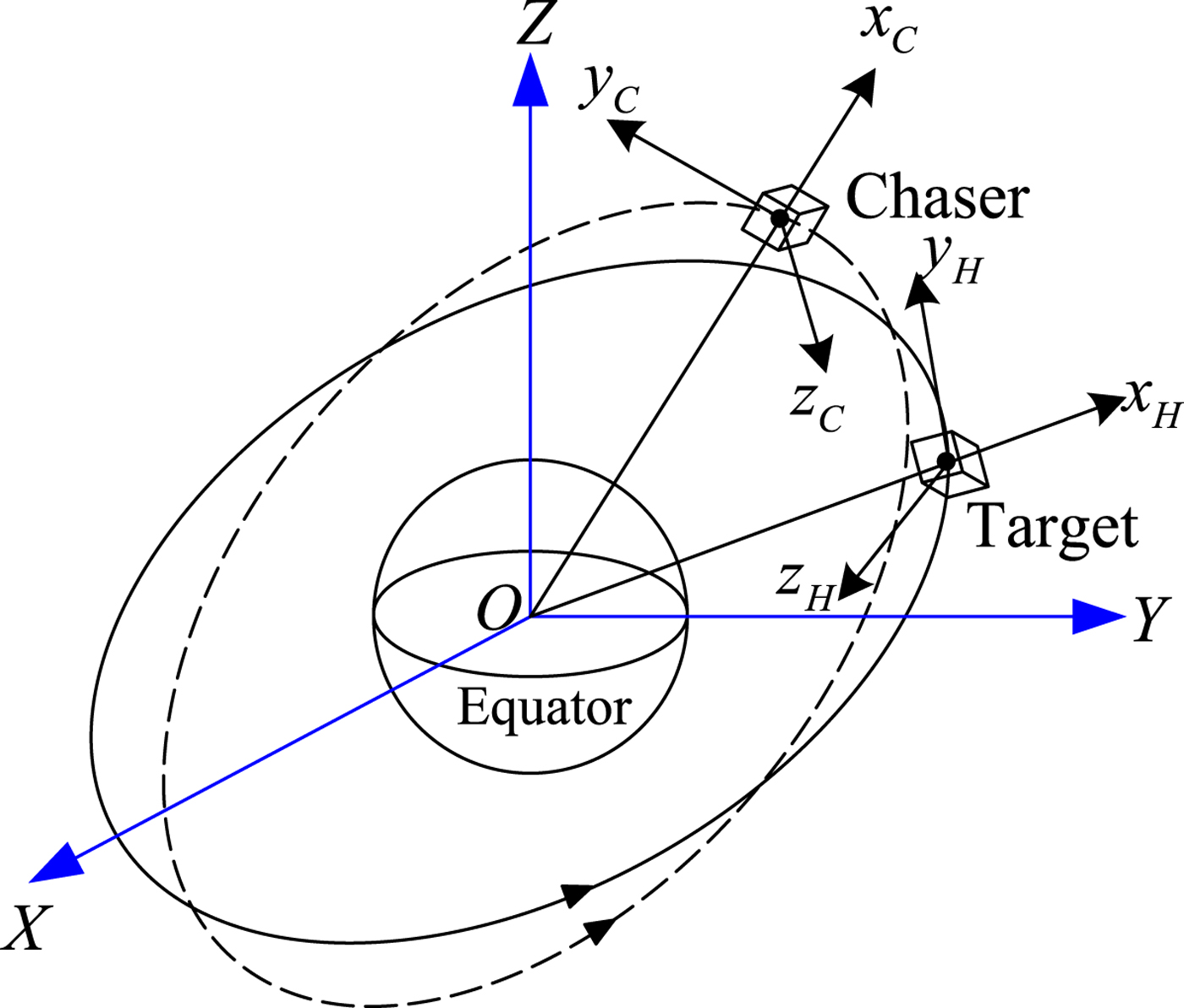
Figure 2. Definitions of various reference frames.

Figure 3. Flyaround plane and nominal flyaround trajectory.

The nominal circular radius is defined as ρ_d, and then quantities ρ_d, θ_y and θ_z can be used to describe the entire nominal trajectory. At time t, the location of the chaser spacecraft can be represented using the phase angle $\gamma =\gamma _{0} +\beta t$ (counter clockwise direction is positive), where $\beta =2\pi /P$ is the flyaround angular velocity and γ₀ is the initial phase angle. Thus, the desired flyaround trajectory can be expressed in the H frame as

(41)$${\bf \rho}_d ={\bi R}_z (-\theta _z){\bi R}_y (-\theta _y)\left[\matrix{ 0 \cr \rho_d \cos (\gamma_0 +\beta t) \cr \rho_d \sin (\gamma_0 +\beta t) }\right]$$

where ${\bi R}_{x} (\cdot)$, ${\bi R}_{y} (\cdot)$, ${\bi R}_{z} (\cdot)$ are the attitude transformation matrices rotating about x, y, z-axes, respectively. They are written as

(42)$$\eqalign{{\bi R}_x (\theta)&=\left[\matrix{ 1 & 0 & 0 \cr 0 & {\cos \theta } & {\sin \theta } \cr 0 & {-\sin \theta } & {\cos \theta } }\right],\quad {\bi R}_y (\theta)=\left[\matrix{ {\cos \theta } & 0 & {-\sin \theta } \cr 0 & 1 & 0 \cr {\sin \theta } & 0 & {\cos \theta } \cr }\right], \cr &\quad {\bi R}_z (\theta)=\left[\matrix{ {\cos \theta } & {\sin \theta } & 0 \cr {-\sin \theta } & {\cos \theta } & 0 \cr 0 & 0 & 1 }\right]}$$

Calculating the first and second derivatives of Equation (41), we have the desired relative velocity and relative acceleration in the H frame as follows:

(43)$$\dot {{\bf \rho} }_d ={\bi R}_z \lpar -\theta_z\rpar {\bi R}_y \lpar -\theta_y\rpar \left[\matrix{ 0 \cr -\beta \rho_d \sin (\gamma_0 +\beta t) \cr \beta \rho_d \cos (\gamma_0 +\beta t)}\right]$$

(44)$$\ddot {{\bf \rho} }_d ={\bi R}_z \lpar {-\theta_z } \rpar {\bi R}_y \lpar {-\theta_y } \rpar \left[\matrix{ 0 \cr {-\beta^2\rho_d \cos \lpar {\gamma_0 +\beta t} \rpar } \cr {-\beta^2\rho_d \sin \lpar {\gamma_0 +\beta t} \rpar }}\right]$$

The desired reference trajectory ${\bi r}_{d}$ expressed in I coordinates is written as

(45)$${\bi r}_d^I ={\bi r}_T +{\bi A}_{H\to I} {\bf \rho}_d$$

where ${\bi r}_{T}$ is the inertial position vector of the target spacecraft and ${\bi A}_{H\to I} $ is the attitude matrix from the H frame to the I frame, which can be expressed as

(46)$${\bi A}_{H\to I} =\left[\matrix{{\bi i}_H & {\bi j}_H & {\bi k}_H}\right]$$

where ${\bi i}_{H} $, ${\bi j}_{H}$ and ${\bi k}_{H}$ are unit vectors of the three axes of the H frame expressed in the I frame, given by

(47)$${\bi i}_H = {{\bi r}_T \over \vert {{\bi r}_T} \vert },\quad {\bi j}_H ={\bi k}_H \times {\bi i}_H ,\quad {\bi k}_H = {{\bf \omega}_{H/I}^I \over \vert {\bf \omega}_{H/I}^I \vert }$$

where ${\bf \omega}_{H/I}^{I} $ is the angular velocity of the target's LVLH frame expressed in the I frame, given by

(48)$${\bf \omega} _{H/I}^I = {{\bi r}_T \times {\bi v}_T \over \vert {\bi r}_T \vert ^2}$$

where ${\bi v}_{T} $ is the inertial velocity vector of the target spacecraft.

In addition, ${\bf \omega} _{H/I}^{H} $ is the angular velocity of the H frame relative to the I frame expressed in H coordinates, that is

(49)$${\bf \omega} _{H/I}^H =\left[\matrix{0 & 0 & \vert{\bf \omega}_{H/I}^I \vert}\right]^T$$

Using Equations (45) and (49), the desired inertial velocity vector $\dot{\bi r}_{d}^{I}$ is computed as

(50)$$\dot{\bi r}_d^I =\dot{\bi r}_T +{\bi A}_{H\to I} \lpar \dot{{\bf \rho}}_d +{\bf \omega}_{H/I}^H \times {\bf \rho}_d\rpar $$

Further, the desired inertial acceleration vector $\ddot{{\bi r}}_{d}^{I}$ is computed as

(51)$$\ddot{{\bi r}}_d^I = \ddot{{\bi r}}_T +{\bi A}_{H\to I} \lcub \ddot{{\bf \rho}}_d +2{\bf \omega}_{H/I}^H \times \dot{{\bf \rho}}_d +\dot{{\bf \omega}}_{H/I}^H \times {\bf \rho}_d +{\bf \omega}_{H/I}^H \times \lpar {\bf \omega}_{H/I}^H \times {\bf \rho}_d\rpar \rcub $$

4.2. In-orbit inspection mission trajectory

For an in-orbit inspection mission, the pointing logic will be that of having an inspection camera mounted on the chaser spacecraft pointing towards the target spacecraft. This we refer to as the inspection mode. Hence, the desired orientation of the chaser spacecraft varies during the inspection mission. The desired angular velocity of the chaser spacecraft is relevant to the orbit angular velocity of the target spacecraft. Thus, the desired inspection mission trajectory consisting of desired attitude, angular velocity and angular acceleration is given.

It is assumed that the inspection camera is mounted on the body +X _C axis of the chaser spacecraft. As illustrated in Figure 4, the inspection camera always points towards the target spacecraft in the inspection mode. Thus, the desired body +X _C -axis needs be opposed to the direction of relative position vector ${\bf \rho}_{d}$.

Figure 4. Inspection mode sketch map.

In the inspection mode, the chaser spacecraft must rotate so that the target spacecraft remains within the field of view of the inspection camera. The desired rotation rate is the rotation rate of ${\bf \rho}_{d}$. Using the concept of instantaneous angular velocity, we obtain the desired angular velocity and angular acceleration as follows:

(52)$${\bf \omega}_{d/H}^H = {{\bf \rho}_d \times \dot{{\bf \rho}}_d \over \vert {\bf \rho}_d \vert^2}$$

(53)$$\dot{{\bf \omega}}_{d/H}^H = {{\bf \rho}_d \times \ddot{{\bf \rho}}_d \over \vert\rho_d \vert^2}$$

where ${\bf \omega}_{d/H}^{H} $ and $\dot{{\bf \omega}}_{d/H}^{H}$ are both expressed in H coordinates.

By definition, the unit vectors of the three axes of the desired frame expressed in H coordinates are given by

(54)$${\bi i}_d =- {{\bf \rho}_d \over \vert {\bf \rho}_d\vert},\quad {\bi j}_{\!d} ={\bi k}_d \times {\bi i}_d ,\quad {\bi k}_d = {{\bf \omega}_{d/H}^H \over \vert{\bf \omega}_{d/H}^H \vert}$$

Then, the attitude matrix from the H frame to the d frame is given by

(55)$${\bi A}_{H\to d} =\left[\matrix{ {{\bi i}_d^T } \cr {{\bi j}_{\!d}^{\!T}} \cr {\bi k}_d^T} \right]$$

The desired relative angular velocity and angular acceleration expressed in d coordinates are computed as

(56)$${\bf \omega}_{d/H}^d =\left[\matrix{0 & 0 & \vert{\bf \omega}_{d/H}^H \vert}\right]^T$$

(57)$$\dot{{\bf \omega}}_{d/H}^d =\left[\matrix{0 & 0 & \vert \dot{{\bf \omega}}_{d/H}^H \vert}\right]^T$$

The attitude matrix from the I frame to the H frame can be obtained by transposing Equation (46), that is

(58)$${\bi A}_{I\to H} =\left[\matrix{{\bi i}_H^T \cr {\bi j}_{H}^{T} \cr {\bi k}_H^T} \right]$$

Combining Equations (55) and (58), we have the attitude matrix from the I frame to the d frame as follows

(59)$${\bi A}_{I\to d} ={\bi A}_{H\to d} {\bi A}_{I\to H}$$

Further, the desired inertial attitude quaternion q_d can be calculated using the attitude matrix A_I→d.

Therefore, the desired inertial angular velocity of the chaser spacecraft is computed as

(60)$${\bf \omega}_{d/I}^d ={\bf \omega}_{d/H}^d +{\bi A}_{H\to d} {\bf \omega}_{H/I}^H$$

4.3. Dual-number-based desired mission trajectory

According to dual-number-based spacecraft kinematics and dynamics models in Section 3, the above space flyaround and inspection mission model based on dual numbers is derived as follows.

By definition, the desired dual quaternion ${\mathop{\bi q}\limits^{\frown}}_{d} $ described in the ECI frame is given by

(61)$${\mathop{\bi q}\limits^{\frown}}_d ={\bi q}_d +\varepsilon {1 \over 2}{\bi q}_d \otimes {\bi r}_d^I$$

The corresponding desired twist ${\mathop{\bf \omega}\limits^{\frown}}_{d/I}^{d}$ is given by

(62)$${\mathop{\bf \omega}\limits^{\frown}}_{d/I}^d = {\bf \omega}_{d/I}^d + \varepsilon \lpar {\bi q}_d \otimes \dot{\bi r}_d^I \otimes {\bi q}_d^{-1} \rpar $$

where q_d, ω_d/I^d, r_d^I and $\dot{\bi r}_{d}^{I}$ have been computed in the previous subsection.

Taking the time derivative of Equation (62) gives the following desired twist acceleration $\dot{\mathop{\bf \omega}\limits^{\frown}}_{d/I}^{d}$

(63)$$\eqalign{\dot{\mathop{\bf \omega}\limits^{\frown}}_{d/I}^d &= \dot{\bf \omega}_{d/I}^d +\varepsilon \lpar \dot{\bi q}_d \otimes \dot{\bi r}_d^I \otimes {\bi q}_d^{-1} +{\bi q}_d \otimes \ddot{\bi r}_d^I \otimes {\bi q}_d^{-1} +\dot{\bi q}_d \otimes \dot{\bi r}_d^I \otimes \dot{\bi q}_d^{-1} \rpar \cr &=\dot{\bf \omega}_{d/I}^d +\varepsilon \left({\bi q}_d \otimes \ddot{\bi r}_d^I \otimes {\bi q}_d^{-1} + {1 \over 2}{\bf \omega}_{d/I}^d \otimes {\bi q}_d \otimes \dot{\bi r}_d^I \otimes {\bi q}_d^{-1} - {1 \over 2} {\bi q}_d \otimes \dot{\bi r}_d^I \otimes {\bi q}_d^{-1} \otimes {\bf \omega}_{d/I}^d \right) \cr & = \dot{\bf \omega}_{d/I}^d +\varepsilon \lpar {\bi q}_d \otimes \ddot{\bi r}_d^I \otimes {\bi q}_d^{-1} +\lpar {\bi q}_d \otimes \dot{\bi r}_d^I \otimes {\bi q}_d^{-1} \rpar \times {\bf \omega}_{d/I}^d \rpar }$$

where the desired angular acceleration $\dot{\bf \omega}_{d/I}^{d}$ can be computed using Equation (60) as follows

(64)$$\dot{\bf \omega}_{d/I}^d = \dot{\bf \omega}_{d/H}^d + {\bi A}_{H\to d} \dot{\bf \omega}_{H/I}^H -{\bf \omega}_{d/H}^d \times {\bi A}_{H\to d} {\bf \omega}_{H/I}^H$$

Hence, the desired dual quaternion ${\mathop{\bi q}\limits^{\frown}}_{d}$, twist ${\mathop{\bf \omega}\limits^{\frown}}_{d/I}^{d}$ and twist acceleration $\dot{\mathop{\bf \omega}\limits^{\frown}}_{d/I}^{d}$ have been formulated using the dual number method.

5.1. PD control system

For the chaser spacecraft, the integrated translational and rotational equations of motion based on dual number have been derived in Section 3. Rewriting Equation (34) leads to

(65)$$\dot{\mathop{\bf \omega}\limits^{\frown}}_{C/I}^C = {\mathop{\bi M}\limits^{\frown}}_C^{-1} \lpar {\mathop{\bi u}\limits^{\frown}}_g^C - {\mathop{\bf \omega}\limits^{\frown}}_{C/I}^C \times {\mathop{\bi M}\limits^{\frown}}_C {\mathop{\bf \omega}\limits^{\frown}}_{C/I}^C \rpar + {\mathop{\bi M}\limits^{\frown}}_C^{-1} {\mathop{\bi u}\limits^{\frown}}_c^C +{\mathop{\bi M}\limits^{\frown}}_C^{-1} {\mathop{\bi d}\limits^{\frown}}$$

This is an integrated orbit and attitude coupled dynamics equation. For conciseness, the adjoint transformation for the unit dual quaternion can be denoted as

(66)$${\mathop{\bi A}\limits^{\frown}}_{\mathop{\bi q}\limits^{\frown}} \mathop{\bi v}\limits^{\frown} \equiv \mathop{\bi q}\limits^{\frown} \otimes \mathop{\bi v}\limits^{\frown} \otimes {\mathop{\bi q}\limits^{\frown}}^{-1} = \mathop{\bi q}\limits^{\frown} \otimes \mathop{\bi v}\limits^{\frown} \otimes {\mathop{\bi q}\limits^{\frown}}^{\ast}$$

The error dual quaternion ${\mathop{\bi q}\limits^{\frown}}_{e} $ between the C and d frames has been defined in Equation (18). According to the desired mission trajectory, the PD control law based on dual numbers can be designed as follows

(67)$$\eqalign{{\mathop{\bi u}\limits^{\frown}}_{\rm PD} & =\underbrace{\lpar {\mathop{\bf \omega}\limits^{\frown}}_{C/I}^C \times {\mathop{\bi M}\limits^{\frown}}_C {\mathop{\bf \omega}\limits^{\frown}}_{C/I}^C - {\mathop{\bi u}\limits^{\frown}}_g^C \rpar + {\mathop{\bi M}\limits^{\frown}}_C \lpar {\mathop{\bi A}\limits^{\frown}}_{{\mathop{\bi q}\limits^{\frown}}_e} \dot{{\mathop{\bf \omega}\limits^{\frown}}}_{d/I}^d -\lsqb {\mathop{\bf \omega}\limits^{\frown}}_{C/I}^C \times \rsqb {\mathop{\bi A}\limits^{\frown}}_{{\mathop{\bi q}\limits^{\frown}}_e} {\mathop{\bf \omega}\limits^{\frown}}_{d/I}^d \rpar }_{-\mathop{g}\limits^{\frown} \lpar {\mathop{\bi M}\limits^{\frown}}_C, {\mathop{\bi q}\limits^{\frown}}_e, {\mathop{\bf \omega}\limits^{\frown}}_{C/d}^C \rpar } \cr &\quad - {\mathop{\bi K}\limits^{\frown}}_p {\mathop{\bf \varrho}\limits^{\frown}}_e - {\mathop{\bi K}\limits^{\frown}}_d \lpar {\mathop{\bf \omega}\limits^{\frown}}_{C/I}^C - {\mathop{\bi A}\limits^{\frown}}_{{\mathop{\bi q}\limits^{\frown}}_e} {\mathop{\bf \omega}\limits^{\frown}}_{d/I}^d \rpar \cr &=-\mathop{\bf g}\limits^{\frown} \lpar {\mathop{\bi M}\limits^{\frown}}_C, {\mathop{\bi q}\limits^{\frown}}_e, {\mathop{\bf \omega}\limits^{\frown}}_{C/d}^C \rpar - {\mathop{\bi K}\limits^{\frown}}_p {\mathop{\bf \varrho}\limits^{\frown}}_e - {\mathop{\bi K}\limits^{\frown}}_d \lpar {\mathop{\bf \omega}\limits^{\frown}}_{C/I}^C - {\mathop{\bi A}\limits^{\frown}}_{{\mathop{\bi q}\limits^{\frown}}_e} {\mathop{\bf \omega}\limits^{\frown}}_{d/I}^d \rpar }$$

where ${\mathop{\bf \varrho}\limits^{\frown}}_{e}$ is the vector part of ${\mathop{\bi q}\limits^{\frown}}_{e}$. The dual control operators ${\mathop{\bi K}\limits^{\frown}}_{p}$ and ${\mathop{\bi K}\limits^{\frown}}_{d}$ have the following form

(68)$$\eqalign{{\mathop{\bi K}\limits^{\frown}}_p &={\bi K}_r {d \over d\varepsilon} + \varepsilon {\bi K}_q \cr {\mathop{\bi K}\limits^{\frown}}_d & ={\bi K}_v {d \over d\varepsilon} + \varepsilon {\bi K}_\omega}$$

where K_r, K_q, K_v and K_ω are to-be-determined proportional and derivative control gains. By the classic control theory, the control parameters are computed as

(69)$${\bi K}_r = m_C \omega _r^2 {\bi I}_{3\times 3}\quad {\bi K}_v = 2m_C \zeta_r \omega_r {\bi I}_{3\times 3}$$

(70)$${\bi K}_q =\omega _\theta ^2 {\bi J}_C \quad {\bi K}_\omega = 2 \zeta_{\theta} \omega _{\theta} {\bi J}_C$$

where ω_r and ζ_r are the desired natural frequency and damping ratio of the translational control system, respectively; ω_θ and ζ_θ are the desired natural frequency and damping ratio of the rotational control system, respectively.

The structure form of the dual-based-number PD control law in Equation (67) is similar to the traditional PD control law for the attitude tracking problem. Thus, the Lyapunov stability demonstration is omitted here for conciseness. Rewriting the PD control law in Equation (67) into real and dual forms, we obtain

(71)$$\left\{\matrix{{\bi f}_c^{\,C} =-{\bi K}_r {\bi p}_{C/d}^C - {\bi K}_v \lpar \dot{\bi p}_{C/d}^C + {\bf \omega}_{C/d}^C \times {\bi p}_{C/d}^C \rpar - {\bi g} \lpar \mathop{\bi M}\limits^{\frown}, {\mathop{\bi q}\limits^{\frown}}_e, {\mathop{\bf \omega}\limits^{\frown}}_{C/d}^C \rpar \hfill \cr {\bf \tau}_c^C = -{\bi K}_q {\bf \varrho}_e -{\bi K}_{\omega} {\bf \omega}_{C/d}^C -{\bf g}^{\prime} \lpar \mathop{\bi M}\limits^{\frown}, {\mathop{\bi q}\limits^{\frown}}_e , {\mathop{\bf \omega}\limits^{\frown}}_{C/d}^C \rpar \hfill} \right.$$

where ${\bi g}\lpar {\mathop{\bi M}\limits^{\frown}}_{C}, {\mathop{\bi q}\limits^{\frown}}_{e}, {\mathop{\bf \omega}\limits^{\frown}}_{C/d}^{C} \rpar $ and ${\bi g}^{\prime} \lpar {\mathop{\bi M}\limits^{\frown}}_{C}, {\mathop{\bi q}\limits^{\frown}}_{e}, {\mathop{\bf \omega}\limits^{\frown}}_{C/d}^{C} \rpar $ are the real and dual parts of $\mathop{\bi g}\limits^{\frown} \lpar {\mathop{\bi M}\limits^{\frown}}_{C}, {\mathop{\bi q}\limits^{\frown}}_{e}, {\mathop{\bf \omega}\limits^{\frown}}_{C/d}^{C} \rpar $, respectively. Compared with the traditional separated orbit and attitude control laws, the proposed PD control law based on dual numbers includes the coupling terms such as ${\bf \omega}_{C/d}^{C} \times {\bi p}_{C/d}^{C}$, which is more reasonable and accurate. Therefore, the control precision of the designed PD control system is better than that of traditional separated control system.

5.2. Variable-structure sliding mode control system

In this section, variable-structure sliding mode control is extended into the dual number area. Consider a dynamic system with the following dual form

(72)$$\dot{\mathop{\bi x}\limits^{\frown}} = {\mathop{\bi f}\limits^{\frown}}({\mathop{\bi x}\limits^{\frown}})+{\mathop{\bi B}\limits^{\frown}}({\mathop{\bi x}\limits^{\frown}}){\mathop{\bi u}\limits^{\frown}}$$

where ${\mathop{\bi x}\limits^{\frown}}$ is a dual state vector, ${\mathop{\bi f}\limits^{\frown}}({\mathop{\bi x}\limits^{\frown}})$ contains the effects of the states on their derivatives, ${\mathop{\bi B}\limits^{\frown}}({\mathop{\bi x}\limits^{\frown}})$ is the dual control gain matrix and ${\mathop{\bi u}\limits^{\frown}}$ is the dual vector of control inputs.

Similar to the traditional VSC law derived in Slotine and Li (Reference Slotine and Li1991), the VSC law based on dual numbers is given by

(73)$${\mathop{\bi u}\limits^{\frown}} = -{\mathop{\bi B}\limits^{\frown}}^{-1} \left[{\mathop{\bi f}\limits^{\frown}} + \dot{\mathop{\bi s}\limits^{\frown}} - {\mathop{\bi x}\limits^{\frown}}^{(n)} + {\mathop{\bi G}\limits^{\frown}} \hbox{sat} \left({\mathop{\bi s}\limits^{\frown} \over \mathop{\rho}\limits^{\frown}} \right)\right]$$

where ${\mathop{\bi s}\limits^{\frown}}$ is a dual sliding vector, ${\mathop{\bi G}\limits^{\frown}}$ and $\mathop{\rho}\limits^{\frown}$ are additional control gains, and “sat” is the saturation function. This expression incorporates the modifications that allow for the trade-off between tracking performance and control activity. The “${\mathop{\bi f}\limits^{\frown}} + \dot{\mathop{\bi s}\limits^{\frown}} - {\mathop{\bi x}\limits^{\frown}}^{(n)}$” term provides the dual sliding mode control. In order to overcome the chattering, the discontinuity across ${\mathop{\bi s}\limits^{\frown}} = {\bf 0}$ is smoothed by forming a thin boundary layer of thickness $\mathop{\rho}\limits^{\frown}$ about the dual sliding surface and is accomplished using the saturation function.

For the space flyaround and in-orbit inspection mission, the dual sliding vector is chosen as

(74)$${\mathop{\bi s}\limits^{\frown}} = \lpar {\mathop{\bf \omega}\limits^{\frown}}_{C/I}^C - {\mathop{\bi A}\limits^{\frown}}_{{\mathop{\bi q}\limits^{\frown}}_e} {\mathop{\bf \omega}\limits^{\frown}}_{d/I}^d \rpar + \mathop{\lambda}\limits^{\frown} {\mathop{\bf \varrho}\limits^{\frown}}_e$$

with

(75)$$\mathop{\lambda}\limits^{\frown} = \lambda_r +\varepsilon \lambda _t$$

where λ_r and λ_t are the control gains for the rotational and translational motions, respectively.

The time derivative of the dual sliding surface is given by

(76)$$\dot{\mathop{\bi s}\limits^{\frown}} = \lsqb \dot{\mathop{\bf \omega}\limits^{\frown}}_{C/I}^C - {\mathop{\bi A}\limits^{\frown}}_{{\mathop{\bi q}\limits^{\frown}}_e} \dot{\mathop{\bf \omega}\limits^{\frown}}_{d/I}^d + \lpar {\mathop{\bf \omega}\limits^{\frown}}_{C/I}^C -{\mathop{\bi A}\limits^{\frown}}_{{\mathop{\bi q}\limits^{\frown}}_e} {\mathop{\bf \omega}\limits^{\frown}}_{d/I}^d \rpar \times {\mathop{\bi A}\limits^{\frown}}_{{\mathop{\bi q}\limits^{\frown}}_e} {\mathop{\bf \omega}\limits^{\frown}}_{d/I}^d \rsqb + \mathop{\lambda}\limits^{\frown} \dot{\mathop{\bf \varrho}\limits^{\frown}}_e$$

where $\dot{\mathop{\bf \varrho}\limits^{\frown}}_{e}$ is the vector part of $\dot{\mathop{\bi q}\limits^{\frown}}_{e}$, and $\dot{\mathop{\bi q}\limits^{\frown}}_{e}$ can be obtained by differentiating Equation (18)

(77)$$\eqalign{\dot{\mathop{\bi q}\limits^{\frown}}_e &= \dot{\mathop{\bi q}\limits^{\frown}}_C \otimes {\mathop{\bi q}\limits^{\frown}}_d^{-1} + {\mathop{\bi q}\limits^{\frown}}_C \otimes \dot{\mathop{\bi q}\limits^{\frown}}_d^{-1} \cr &= {1 \over 2} {\mathop{\bf \omega}\limits^{\frown}}_{C/I}^C \otimes {\mathop{\bi q}\limits^{\frown}}_C \otimes {\mathop{\bi q}\limits^{\frown}}_d^{-1} - {1 \over 2} {\mathop{\bi q}\limits^{\frown}}_C \otimes {\mathop{\bi q}\limits^{\frown}}_d^{-1} \otimes {\mathop{\bf \omega}\limits^{\frown}}_{d/I}^d}$$

It is seen from Equation (77) that $\dot{\mathop{\bi q}\limits^{\frown}}_{e}$ can be described using the desired twist ${\mathop{\bf \omega}\limits^{\frown}}_{d/I}^{d}$ and desired dual quaternion ${\mathop{\bi q}\limits^{\frown}}_{d}$, and the current twist ${\mathop{\bf \omega}\limits^{\frown}}_{C/I}^{C}$ and dual quaternion ${\mathop{\bi q}\limits^{\frown}}_{C}$ of the chaser spacecraft.

According to Equation (65), ${\mathop{\bi f}\limits^{\frown}}$ and ${\mathop{\bi B}\limits^{\frown}}$ are given by

(78)$$\eqalign{{\mathop{\bi f}\limits^{\frown}} & ={\mathop{\bi M}\limits^{\frown}}_C^{-1} \lpar {\mathop{\bi u}\limits^{\frown}}_g^C - {\mathop{\bf \omega}\limits^{\frown}}_{C/I}^C \times {\mathop{\bi M}\limits^{\frown}}_C {\mathop{\bf \omega}\limits^{\frown}}_{C/I}^C \rpar \cr {\mathop{\bi B}\limits^{\frown}} & = {\mathop{\bi M}\limits^{\frown}}_C^{-1}}$$

Substituting Equations (74), (76) and (78) into Equation (73) gives the following VSC law

(79)$${\mathop{\bi u}\limits^{\frown}}_{\rm VSC} = \lpar {\mathop{\bf \omega}\limits^{\frown}}_{C/I}^C \times {\mathop{\bi M}\limits^{\frown}}_C {\mathop{\bf \omega}\limits^{\frown}}_{C/I}^C -{\mathop{\bi u}\limits^{\frown}}_g^C \rpar + {\mathop{\bi M}\limits^{\frown}}_C \left\{{\mathop{\bi A}\limits^{\frown}}_{{\mathop{\bi q}\limits^{\frown}}_e} \dot{\mathop{\bf \omega}\limits^{\frown}}_{d/I}^d -\lsqb {\mathop{\bf \omega}\limits^{\frown}}_{C/I}^C \times \rsqb {\mathop{\bi A}\limits^{\frown}}_{{\mathop{\bi q}\limits^{\frown}}_e} {\mathop{\bf \omega}\limits^{\frown}}_{d/I}^d - \mathop{\lambda}\limits^{\frown} \dot{{\mathop{\bf \varrho}\limits^{\frown}}}_e - {\mathop{\bi G}\limits^{\frown}} \hbox{sat} \left({{\mathop{\bi s}\limits^{\frown}} \over {\mathop{\bf \rho}\limits^{\frown}}} \right)\right\}$$

with

(80)$$\eqalign{{\mathop{\bi G}\limits^{\frown}} & = {\bi G}_r + \varepsilon {\bi G}_t \cr \mathop{\rho}\limits^{\frown} & =\rho_r + \varepsilon \rho_t}$$

where G_r and G_t are 3×3 positive definite diagonal matrices and ρ_r and ρ_t are the boundary layer thicknesses for the rotational and translational motions, respectively.

6.1. Desired mission trajectory

It is assumed that the target spacecraft runs on an orbit with an inclination of 0° and a height of 500 km. The distance from the Earth's centre to the target spacecraft is r _T=6, 871 km, and the orbit angular velocity is given by $n_{T} = \sqrt{u/r_{T}^{3}}$. The inertial position, velocity and acceleration vectors of the target spacecraft are written as

(81)$${\bi r}_T = r_T \left[\matrix{\cos (n_T t) \cr \sin (n_T t)\cr 0} \right], \quad \dot{\bi r}_T = r_T n_T \left[\matrix{ -\sin (n_T t) \cr \cos (n_T t) \cr 0} \right], \quad \ddot{\bi r}_T = -r_T n_T^2 \left[\matrix{\cos (n_T t) \cr \sin (n_T t) \cr 0} \right]$$

where gravitational constant μ is given as $3.986 \times 10^{14}\,\hbox{m}^{3}/\hbox{s}^{2}$, and t is the flyaround time.

The angular velocity of the H frame relative to the I frame is given by

(82)$${\bf \omega}_{H/I}^H = [\matrix{0 & 0 & n_T}]^T$$

From Equation (46), the attitude matrix from the H frame of the target spacecraft to the I frame is given by

(83)$${\bi A}_{H\to I} = \left[\matrix{\cos (n_T t) & - \sin (n_T t) &0 \cr \sin (n_T t) & \cos (n_T t) & 0 \cr 0 & 0 & 1} \right]$$

The nominal flyaround trajectory parameters are given by ρ_d=100 m, θ_y=0°, θ_z=0° and γ₀=0°. The flyaround period P is 10 minutes. Thus, the position, velocity and acceleration of the desired flyaround trajectory expressed in the H frame are given by

(84)$${\bf \rho}_d = \left[\matrix{ 0 \cr \rho_d \cos (\beta t) \cr \rho_d \sin (\beta t)} \right], \quad \dot{\bf \rho}_d = \left[\matrix{0 \cr -\beta \rho_d \sin (\beta t) \cr \beta \rho_d \cos (\beta t)} \right], \quad \ddot{\bf \rho}_d =\left[\matrix{0 \cr - \beta^2 \rho_d \cos (\beta t) \cr -\beta^2 \rho_d \sin (\beta t)} \right]$$

where β=2π/P is the flyaround angular velocity.

Using Equations (45), (50) and (51), we can obtain the desired inertial position, velocity and acceleration of the chaser spacecraft. The detailed derivations are omitted here for conciseness. According to the in-orbit inspection requirements, the desired relative angular velocity and acceleration expressed in d coordinates are given by

(85)$${\bf \omega}_{d/H}^d = [\matrix{0 & 0 & \beta}]^T, \quad \dot{\bf \omega}_{d/H}^d = [\matrix{0 & 0 & 0}]^T$$

The unit vectors of the three axes of the desired frame expressed in H coordinates are computed as

(86)$${\bi i}_d = \left[\matrix{0 \cr -\cos (\beta t) \cr -\sin (\beta t)} \right], \quad {\bi j}_d = \left[\matrix{ 0 \cr \sin (\beta t) \cr -\cos (\beta t)} \right], \quad {\bi k}_d = \left[\matrix{1 \cr 0 \cr 0} \right]$$

Thus, the attitude matrix from the H frame to the d frame is calculated using Equation (55) as follows

(87)$${\bi A}_{H\to d} = \left[\matrix{0 & - \cos (\beta t) &-\sin (\beta t) \cr 0 & \sin (\beta t) & -\cos (\beta t) \cr 1 & 0 & 0} \right]$$

The desired inertial angular velocity of the chaser spacecraft can be computed using Equation (60) as

(88)$${\bf \omega}_{d/I}^d = {\bf \omega}_{d/H}^d + {\bi A}_{H\to d} {\bf \omega}_{H/I}^H = \left[\matrix{-n_T \sin (\beta t) \cr - n_T \cos (\beta t) \cr \beta} \right]$$

Further, the desired inertial angular acceleration is given by

(89)$$\dot{\bf \omega}_{d/I}^d = \left[\matrix{-\beta n_T \cos (\beta t) \cr \beta n_T \sin (\beta t) \cr 0} \right]$$

The desired twist ${\mathop{\bf \omega}\limits^{\frown}}_{d/I}^{d}$ and desired twist acceleration $\dot{\mathop{\bf \omega}\limits^{\frown}}_{d/I}^{d}$ can be obtained using Equations (62) and (63), respectively. Hence, the desired trajectory ${\mathop{\bi q}\limits^{\frown}}_{d}$ can be propagated using Equation (16).

6.2. Numerical simulations

In this section, simulation results are presented that show the effectiveness of the proposed two control systems. The nominal mass of the chaser spacecraft is $\bar{m}=100\,\hbox{kg}$, the mass uncertainty is Δ m=5 kg. The nominal inertia matrix and inertia matrix uncertainty are given by

(90)$$\overline{\bi J}_{C} = \left[\matrix{30 &10 & 5 \cr 10 &20 & 3 \cr 5 & 3 &15} \right]\,\hbox{kg}\;\hbox{m}^{2} \quad \Delta {\bi J}_C = \left[\matrix{6 & 0 & 0 \cr 0 & 4 & 0 \cr 0 & 0 & 3} \right]\,\hbox{kg}\;\hbox{m}^{2}$$

The dual disturbance force vector is given by

(91)$${\mathop{\bi d}\limits^{\frown}} = \left[\matrix{0.001 &0.001 &0.001} \right]^T \sin \lpar n_T t \rpar + \varepsilon \left[\matrix{0.005 &0.005 &0.005} \right]^T \sin \lpar n_T t \rpar $$

The initial conditions are given as follows:

$$t_0 =0\,\hbox{s}, \quad {\bi e}_0 = [\matrix{-3 & 5 &-2}]^T \hbox{m}, \quad \dot {\bi e}_0 = [\matrix{0.002 &0.004 &-0.001}]^T \hbox{m/s}$$

where e₀ and $\dot{\bi e}_0$ are initial position and velocity errors of the flyaround spacecraft, respectively. The simulation time is one flyaround period. The corresponding control system parameters are listed in Table 1.

Table 1. Control system parameters.

Figure 5 shows the flyaround control trajectory. Figures 6 and 8 show the velocity and position tracking errors, respectively. Figures 7 and 9 show the corresponding partial enlargement drawings, respectively. Figures 10 and 12 show the angular velocity and quaternion tracking errors, respectively. Figures 11 and 13 show the corresponding partial enlargement drawings, respectively. Figures 14 and 15 show the control accelerations and control torques, respectively.

Figure 5. Flyaround control trajectory.

Figure 6. Velocity tracking errors.

Figure 7. Partial enlargement drawing of velocity tracking errors.

Figure 8. Position tracking errors.

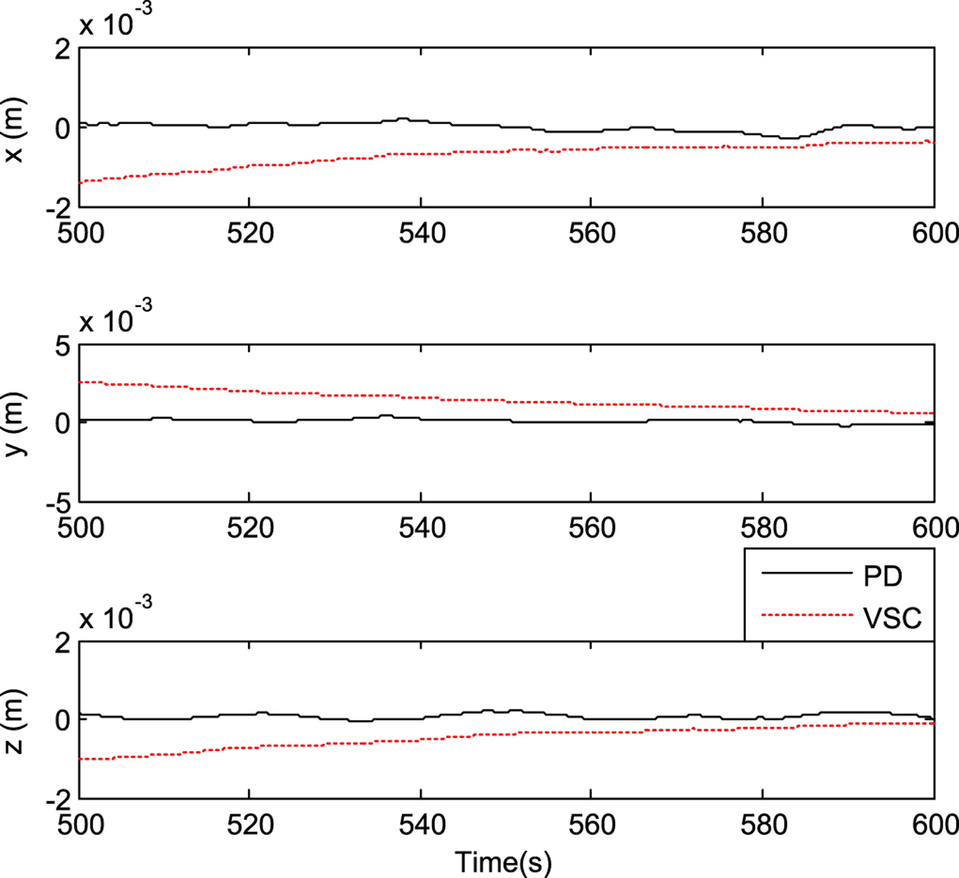
Figure 9. Partial enlargement drawing of position tracking errors.

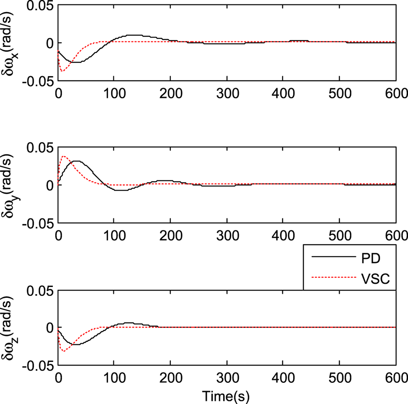
Figure 10. Angular velocity tracking errors.

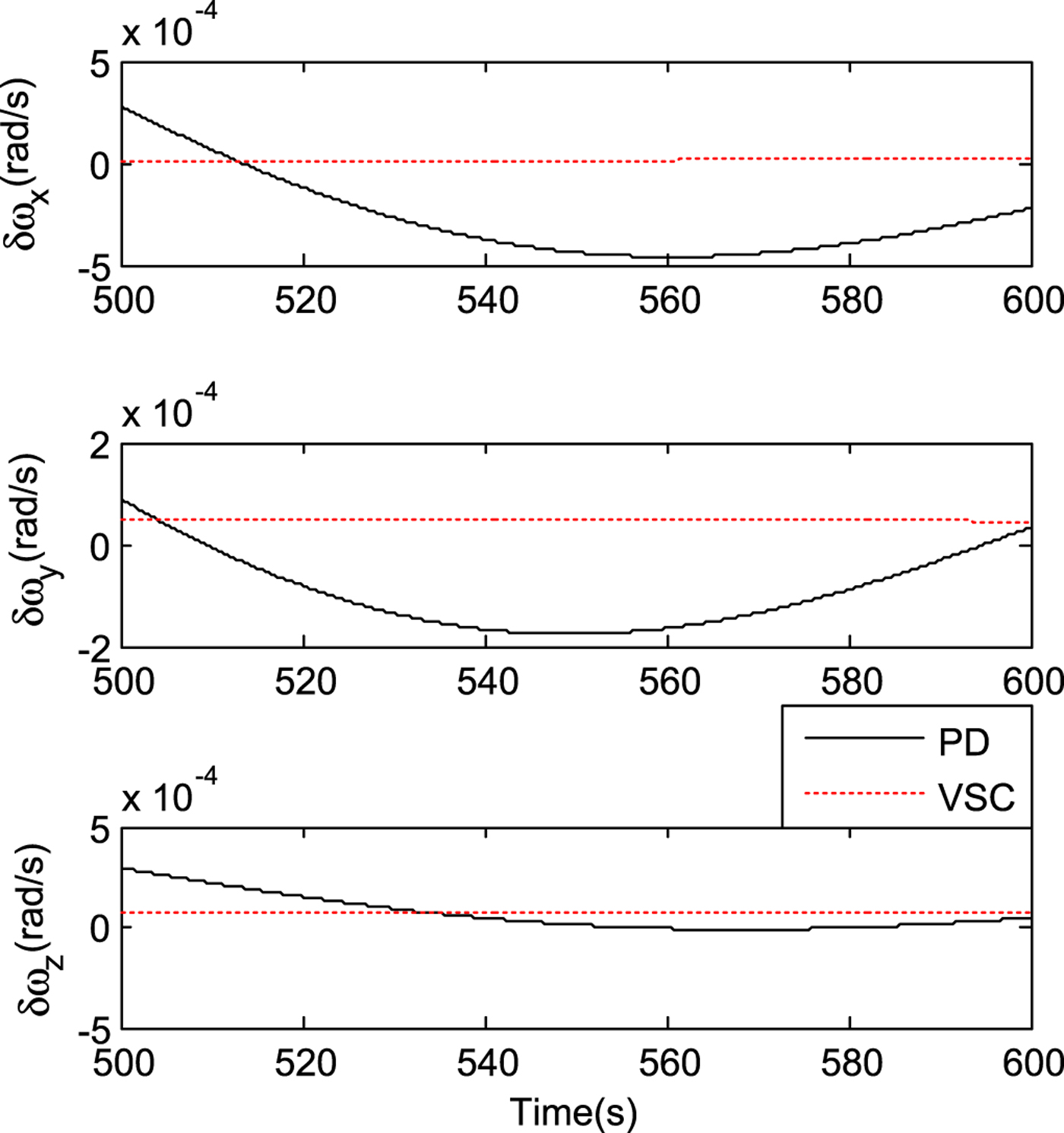
Figure 11. Partial enlargement drawing of angular velocity tracking errors.

Figure 12. Quaternion tracking errors.

Figure 13. Partial enlargement drawing of quaternion tracking errors.

Figure 14. Control acceleration curve.

Figure 15. Control torque curve.

As seen from Figures 6–15, both control approaches are effective, and the tracking errors can converge to zero with the mass and inertia matrix uncertainties. Compared with the PD control system, the sliding mode control system has much higher precision and convergence speed.