


1. INTRODUCTION
Global Navigation Satellite Systems (GNSS) such as the Global Positioning System (GPS) or the future European Galileo system can deliver accurate position information for users worldwide. However, due to the design of GNSS, these state-of-the-art navigation systems are not available for deep space targets. With the expansion of space exploration to the Moon and beyond, the demand for a high-precision cislunar navigation system is becoming increasingly prominent. Considering the existence of periodic motions around the Earth-Moon libration points, a novel navigation architecture consisting of libration point satellites could be a potential solution for autonomous navigation in cislunar space.
The concept of using Earth-Moon libration point satellites for cislunar navigation was first proposed by Farquhar and then followed by many other researchers. Farquhar (Reference Farquhar1967) described the idea of using an Earth-Moon L 2 libration point satellite to provide navigation capability for the far side of the Moon. Grebow (Reference Grebow2006) created architectures for continuous lunar south pole coverage by two satellites located in quasi-periodic orbits around the Earth-Moon L 1 and L 2. Romagnoli and Circi (Reference Romagnoli and Circi2010) investigated Lissajous orbits around the Earth-Moon collinear libration points to realise a Lunar Global Positioning System (LGPS), and later in Circi et al. (Reference Circi, Romagnoli and Fumenti2014), the results were extended to halo orbits. Considering the strong asymmetry of the three-body force field, Hill et al. (Reference Hill, Lo and Born2005a; Reference Hill, Born and Lo2005b) proposed a linked, autonomous orbit determination technique, known as “Liaison Navigation”. Using scalar Satellite-to-Satellite Tracking (SST) data, orbits of the libration point navigation satellites can be determined autonomously. A detailed study on the autonomous orbit determination of libration point satellites can be found in Hill's PhD dissertation (Hill, Reference Hill2007). Based on the Liaison technique, a systematic study of using libration point satellites to construct an autonomous cislunar navigation system was presented in Zhang and Xu (Reference Zhang and Xu2014), where some candidate three-satellite and four-satellite navigation architectures were obtained based on a comprehensive consideration of coverage ability and autonomous orbit determination performance. Subsequent works carried out by Gao et al. (Reference Gao, Xu and Zhang2014) and Zhang and Xu (Reference Zhang and Xu2015) verified the autonomy and feasibility of the Universe Lighthouse.
By noting the probable existence of a simplified constellation architecture for the libration point satellite navigation system, this paper focuses on a detailed investigation of the Earth-Moon L 1,2 two-satellite constellation, which consists of only two navigation satellites located around the Earth-Moon collinear libration points. In order to determine the feasible two-satellite constellations that can achieve continuous global coverage for lunar orbits, an exhaustive search over all possible combinations of Libration Point Orbits (LPOs) is performed first. After finding a set of candidate constellation configurations, a polynomial fitting method is used to derive the amplitude relations between the feasible L 1 and L 2 LPOs. Finally, with the introduction of a reference mission scenario, cislunar navigation performance of the simplified libration point satellite navigation system is verified by Monte Carlo (MC) simulations.
The remainder of this paper is organised as follows. In Section 2, a brief description of the libration point satellite navigation system is given, including the dynamical model and libration point orbits. After discussing the constellation coverage, a thorough search is conducted in Section 3 to determine the feasible two-satellite constellations. After that, Section 4 presents a cislunar navigation simulation to verify the availability of the simplified libration point satellite navigation system. Finally, some brief conclusions are drawn in Section 5.
2. LIBRATION POINT SATELLITE NAVIGATION SYSTEM
The libration point satellite navigation system is a novel navigation architecture that consists of satellites located in periodic orbits around the Earth-Moon libration points. The basic dynamical model is the Circular Restricted Three-Body Problem (CRTBP), which can be expressed in a general form as (Szebehely, Reference Szebehely1967)
 $$\left\{ \matrix{\ddot x = 2\dot y + x - \left( {1 - \mu} \right)\displaystyle{{x + \mu} \over {R_1^3}} - \mu \displaystyle{{x - 1 + \mu} \over {R_2^3}} \hfill \cr \ddot y = - 2\dot x + y - \left( {1 - \mu} \right)\displaystyle{y \over {R_1^3}} - \mu \displaystyle{y \over {R_2^3}} \hfill \cr \ddot z = - \left( {1 - \mu} \right)\displaystyle{z \over {R_1^3}} - \mu \displaystyle{z \over {R_2^3}} \hfill} \right.$$
where μ is the mass parameter of the Earth-Moon system; R 1 and R 2 are the distances from the spacecraft to the Earth and the Moon, respectively.
The equations of motion of the CRTBP allow the existence of five well-known equilibrium points in the synodic coordinate system (as shown in Figure 1). The five equilibrium points, also known as the libration points, are all located in the plane of motion of the primaries, with three collinear ones L 1,2,3 located on the X-axis, and two triangular ones L 4,5 forming two equilateral triangles with the primaries.

Figure 1. Libration points of CRTBP in the Earth-Moon synodic coordinate system.
The dynamics of the CRTBP also predicts the existence of periodic and quasi-periodic orbits around the Earth-Moon libration points. Generally, there are three common classifications of LPOs: Lissajous orbits, Lyapunov orbits, and Halo orbits. A Lissajous orbit is a quasi-periodic trajectory that winds around a torus. Lyapunov orbits are a special case of periodic Lissajous orbits, as the in-plane or out-of-plane amplitude equals zero. Halo orbits are three-dimensional periodic orbits which bifurcate from the planar Lyapunov family (Gómez et al., Reference Gómez, Llibre, Martínez and Simó2001). Using the Lindstedt-Poincaré (L-P) method, analytical expressions for these LPOs can be obtained by series expansion. Below are summarised without derivation the resulting expressions. The construction detail and meanings of coefficients can be found in Lei et al. (Reference Lei, Xu, Hou and Sun2013).
 $$Lissajous: \left\{ \matrix{x\left( t \right) = \sum\limits_{i,\, j = 1}^\infty {\left( {\sum\limits_{\left \vert k \right \vert \le i,\left \vert m \right \vert \le j} {x_{ijkm} \cos \left( {k\theta _1 + m\theta _2} \right)}} \right)} \alpha ^i \beta ^j \hfill \cr y\left( t \right) = \sum\limits_{i,\, j = 1}^\infty {\left( {\sum\limits_{\left \vert k \right \vert \le i,\left \vert m \right \vert \le j} {y_{ijkm} \sin \left( {k\theta _1 + m\theta _2} \right)}} \right)} \alpha ^i \beta ^j \hfill \cr z\left( t \right) = \sum\limits_{i,\,j = 1}^\infty {\left( {\sum\limits_{\left \vert k \right \vert \le i,\left \vert m \right \vert \le j} {z_{ijkm} \cos \left( {k\theta _1 + m\theta _2} \right)}} \right)} \alpha ^i \beta ^j \hfill} \right.$$
 $$Halo: \left\{ \matrix{x\left( t \right) = \sum\limits_{i,\,j = 1}^\infty {\left( {\sum\limits_{\left \vert k \right \vert \le i + j} {x_{ijk} \cos \left( {k\theta} \right)}} \right)} \alpha ^i \beta ^j \hfill \cr y\left( t \right) = \sum\limits_{i,\, j = 1}^\infty {\left( {\sum\limits_{\left \vert k \right \vert \le i + j} {y_{ijk} \sin \left( {k\theta} \right)}} \right)} \alpha ^i \beta ^j \hfill \cr z\left( t \right) = \sum\limits_{i,\, j = 1}^\infty {\left( {\sum\limits_{\left \vert k \right \vert \le i + j} {z_{ijk} \cos \left( {k\theta} \right)}} \right)} \alpha ^i \beta ^j \hfill} \right.$$
It should be noted that when the in-plane amplitude α = 0 in Equation (2), the Lissajous orbits reduce to the vertical Lyapunov orbits and when the out-of-plane amplitude β = 0, they reduce to the planar Lyapunov orbits. Typical plots of LPOs around the Earth-Moon collinear libration point are shown in Figure 2.

Figure 2. Typical plots of LPOs around the Earth-Moon collinear libration point. Upper left: Lissajous orbit. Upper right: planar Lyapunov orbit. Lower left: vertical Lyapunov orbit. Lower right: Halo orbit.
Due to the special location of LPOs, a novel navigation architecture based on libration point satellites can be developed in cislunar space. A major advantage of this system is that the number of satellites needed to achieve continuous global coverage for lunar orbits can be greatly reduced. Besides that, considering the strong asymmetry of the three-body force field, the Liaison technique can be adopted by libration point navigation satellites. In this way, extensive Earth-based tracking measurement can be eliminated, and an autonomous satellite navigation system can be developed. Our previous work has indicated that the Earth-Moon L 2,4,5 three-satellite constellation and the Earth-Moon L 1,2,4,5 four-satellite constellation are feasible architectures for the libration point satellite navigation system. By recognising the probable existence of a simpler constellation configuration, this paper focuses on a detailed investigation of the Earth-Moon L 1,2 two-satellite constellation, especially for its coverage ability and cislunar navigation performance.
3. ARCHITECTURE ANALYSIS OF THE SIMPLIFIED CONSTELLATION
The Earth-Moon L 1,2 two-satellite constellation is the simplest configuration for the libration point satellite navigation system. With only two navigation satellites operating in periodic orbits around the Earth-Moon L 1 and L 2 libration points, coverage ability of this simplified constellation is slightly worse than the three-satellite and four-satellite constellations. However, by selecting an appropriate combination of LPOs, it is still possible to develop a viable navigation architecture in cislunar space. The main objective of this section is to determine the feasible Earth-Moon L 1,2 two-satellite constellations that can achieve continuous global coverage for lunar orbits.
3.1. Candidate Configurations
According to the LPOs existing around the collinear libration points, nine candidate configurations are considered in this work for the Earth-Moon L 1,2 two-satellite constellation. Nominal orbits and constellation types of the candidate configurations are summarised in Table 1.
Table 1. Candidate configurations for the Earth-Moon L 1,2 two-satellite constellation.

It should be noted that only periodic orbits around the collinear libration points are selected as candidate orbits for navigation satellites. This is due to the requirement of a repeatable constellation configuration to ensure continuous coverage for lunar users.
3.2. Constellation Coverage Analysis
Constellation coverage performance is regarded as a primary criterion for navigation constellation design. As the proposed system is primarily designed for cislunar navigation, the coverage here is specific to lunar orbits.
Consider a lunar orbiter moving on a circular orbit, with inclination i and right ascension of the ascending node Ω. The position vector of the lunar orbiter at a given time can be expressed in a Moon-Centred Inertial (MCI) frame as
 $${\bi r}_{MCI} = r\left( {\matrix{ {\cos \Omega \cos u - \cos i\sin \Omega \sin u} \cr {\sin \Omega \cos u + \cos i\cos \Omega \sin u} \cr {\sin i\sin u} \cr}} \right)$$
where r is the orbital radius of the circular orbit, u is the argument of latitude at the given time.
As the position of a libration point navigation satellite is customarily expressed in the Earth-Moon barycentric synodic frame, a coordinate transformation is needed to convert the above lunar orbit to the same frame as navigation satellites. The rotation matrix from the MCI frame to the Moon-centred rotating frame, denoted by
 ${\bf R}_{\bf z} {\bf (t)}$
, is given by
${\bf R}_{\bf z} {\bf (t)}$
, is given by
 $${\bf R}_{\bf z} {\bf (t)} = \left( {\matrix{ {\cos t} & {\sin t} & 0 \cr { - \sin t} & {\cos t} & 0 \cr 0 & 0 & 1 \cr}} \right)$$
It has been assumed that the two frames coincide at t = 0, and the transformation time t is in the normalised unit so as to simplify the rotation matrix to the above form. Then the coordinate transformation from the MCI frame to the Earth-Moon barycentric synodic frame can be expressed as
 $${\bi r}_{syn} = \left( {1 - \mu} \right) \cdot \left( {\matrix{ 1 \cr 0 \cr 0 \cr}} \right) + {\bf R}_{\bf z} {\bf (t)} \cdot {\bi r}_{MCI} $$
where r syn is the position vector expressed in the synodic frame, and μ is the mass parameter of the Earth-Moon system. Substitute the expression of r MCI into the above equation, it can be deduced, after some calculations, that
 $${\bi r}_{syn} = \left( {1 - \mu} \right)\left( {\matrix{ 1 \cr 0 \cr 0 \cr}} \right) + r^{\prime}\left( {\matrix{ {\cos \left( {\Omega - t} \right)\cos kt - \cos i\sin\, \left( {\Omega - t} \right)\sin kt} \cr {\sin \left( {\Omega - t} \right)\cos kt - \cos i\cos\, \left( {\Omega - t} \right)\sin kt} \cr {\sin i\sin kt} \cr}} \right)$$
where r′ is the normalised orbital radius of the circular orbit, k is a scaling factor between the argument of latitude u and normalised time t, which is defined by
 $$u = kt, k = \sqrt {\displaystyle{\mu \over {r^{{\prime}^3}}}} $$
Comparing the second term on the right side of Equation (7) with the expression of
 ${\mathop{r}\limits^{\rightharpoonup}} _{MCI} $
given by Equation (4), it can be found that the right ascension of the ascending node is varying with time in the synodic frame, which means a circular lunar orbit in the MCI frame becomes a selenocentric spherical zone looking from the synodic frame. Besides, it can also be deduced that the size and shape of different spherical zones are only related to the orbital radius and inclination of lunar orbits. When two lunar orbits have the same orbital radius, the spherical zone of the more inclined one will cover the spherical zone with smaller inclination. Consequently, the constraint of continuous global coverage for lunar orbits becomes the equivalent coverage to complete spherical zones in the synodic frame.
${\mathop{r}\limits^{\rightharpoonup}} _{MCI} $
given by Equation (4), it can be found that the right ascension of the ascending node is varying with time in the synodic frame, which means a circular lunar orbit in the MCI frame becomes a selenocentric spherical zone looking from the synodic frame. Besides, it can also be deduced that the size and shape of different spherical zones are only related to the orbital radius and inclination of lunar orbits. When two lunar orbits have the same orbital radius, the spherical zone of the more inclined one will cover the spherical zone with smaller inclination. Consequently, the constraint of continuous global coverage for lunar orbits becomes the equivalent coverage to complete spherical zones in the synodic frame.
According to the above description, coverage of an Earth-Moon L 1,2 two-satellite constellation is analysed through the following steps:
Step I: Compute the spherical zone of a target lunar orbit.
For a given lunar orbit with inclination i and orbital radius r′, the spherical zone in the synodic frame is computed using the following equation:
 $${\bi r}_{sph} = \left( {\matrix{ {1 - \mu + r^{\prime}\cos \beta \cos \alpha} \cr {r^{\prime}\cos \beta \sin \alpha} \cr {r^{\prime}\sin \beta} \cr}} \right), \alpha \in \left[ {0, 2\pi} \right], \beta \in \left[ { - i, i} \right]$$
which determines the target region for coverage analysis.
Step II: Construct the Earth-Moon L 1,2 two-satellite constellation.
Using the analytical expressions for LPOs around the collinear libration points, orbits of the candidate Earth-Moon L 1,2 two-satellite constellation can be constructed and the specific parameters are orbit amplitudes (α or β in Equation (2) and Equation (3)) of libration point satellites.
Step III: Determine the continuous coverage region.
In this step, the continuous coverage region is determined by a thorough search. For every point on the spherical zone, it is specified that only those which can be continuously covered by a libration point satellite are defined as continuous coverage regions. Here, if we denote the target point, the barycentre of the Moon and an arbitrary point on a LPO as T, M, and L, respectively, then the continuous coverage condition can be expressed as
 $$\forall L\,on\,a\,LPO: \angle LMT \lt \theta _1 + \theta _2 = \arccos \left( {\displaystyle{{R_{Moon}} \over {\overline {LM}}}} \right) + \arccos \left( {\displaystyle{{R_{Moon}} \over {\overline {TM}}}} \right)$$
where R Moon is the radius of the Moon and a detailed view of the above relation is shown in Figure 3. Based on this criterion, continuous coverage regions of L 1 and L 2 navigation satellites can be determined respectively and the sum of these regions is defined as the final coverage of the two-satellite constellation.

Figure 3. Illustration of the continuous coverage condition.
Figure 4 illustrates the coverage of a Halo-Halo constellation determined by the above process. The target orbit is a lunar polar orbit with an altitude of 200 km and orbit amplitudes for the L 1 and L 2 navigation satellites are 11603 km and 3870 km, respectively. It is apparent from the figure that there are some regions (α ≈ 90° and α ≈ 270°) which cannot be continuously covered by the given Earth-Moon L 1,2 two-satellite constellation. However, this is not a general conclusion, as can be seen in Figure 5 where the constellation type is changed to a Halo-PL configuration and the blind areas do not exist anymore. Therefore it may be concluded that the coverage is directly related to the constellation type and there do exist feasible Earth-Moon L 1,2 two-satellite constellations that can achieve continuous coverage for lunar orbits.

Figure 4. Coverage performance of a Halo-Halo two-satellite constellation. Left: spherical zone of a lunar polar orbit. Right: planar projection of the spherical zone. The red parts in the figure represent the regions which cannot be continuously covered by the libration point satellites, while the green parts and blue parts represent the regions that can be continuously covered by one libration point satellite and two libration point satellites, respectively.

Figure 5. Coverage performance of a Halo-PL two-satellite constellation. Left: spherical zone of a lunar polar orbit. Right: planar projection of the spherical zone. The meanings of colors are the same as those in Figure 4.
3.3. Feasible Two-Satellite Constellations
For target lunar orbits with inclination i and altitude h, varying in the range of
 $$i \in \left[ {0^{\% \circ}, 90^{\% \circ}} \right], h \in \left[ {100{\rm km}, 2000{\rm km}} \right]$$
constellation coverage of the nine candidate configurations is investigated separately according to the above process. After a thorough search, some feasible two-satellite constellations are obtained and amplitude relations between the feasible L 1 and L 2 LPOs are partially illustrated in Figure 6.

Figure 6. Amplitude relations of some feasible two-satellite constellations. Upper left: Halo-PL constellation. Upper right: Halo-VL constellation. Lower left: PL-Halo constellation. Lower right: PL-PL constellation.
It can be seen from Figure 6 that there exists an amplitude boundary for the feasible L 1 and L 2 LPO combination. Only those two-satellite constellations satisfying the amplitude constraint can fulfil the continuous coverage requirement. In order to express the boundary quantitatively, a polynomial fitting method is employed. With the amplitude of the L 1 LPO as the independent variable, the maximum feasible amplitude for the L 2 navigation satellite can then be approximated by a quadratic polynomial as
 $$\left( {A_2} \right)_{\max} = c_0 + c_1 \cdot A_1 + c_2 \cdot A_1^2 $$
where c 0, c 1 and c 2 are fitting coefficients determined by least-squares regression. In this way, the amplitude constraint for the feasible two-satellite constellations can be obtained and the final results are summarised in Table 2.
Table 2. Amplitude constraints for the feasible Earth-Moon L 1,2 two-satellite constellations.

* For the Halo-Halo constellation, the minimum altitude of a continuous covered lunar orbit is 212 km.
Once the above conditions are satisfied, the corresponding Earth-Moon L 1,2 two-satellite constellations can achieve continuous global coverage for lunar orbits in the given range. But there is one exception: Halo-Halo constellation, which can only achieve continuous global coverage for lunar orbits with altitude larger than 212 km. In the following section, a cislunar navigation simulation will be conducted to further verify the feasibility of the simplified constellations.
4. CISLUNAR NAVIGATION SIMULATION AND RESULTS
4.1. Reference Mission Scenario
The reference lunar exploration mission considered in this work mainly consists of two operation phases: a trans-lunar cruise phase and a lunar orbit phase. The trans-lunar cruise departs from a LEO parking orbit with the orbital parameters given in Table 3.
Table 3. Orbital parameters of the initial LEO parking orbit.
The initial epoch of the mission is defined as 1 January 2025 UTC. By performing an approximately 3·12 km/s manoeuvre in the along-track direction, the spacecraft is inserted into the trans-lunar cruise trajectory at 1 January 2025 08:03:05 UTC. After approximately three days of cruise, the spacecraft reaches perilune at 4 January 2025 07:48:11 UTC with an altitude of 444 km. Then a Lunar orbit insertion (LOI) manoeuvre is performed to insert the spacecraft into a circular, polar lunar orbit. The magnitude of LOI is approximately 854 m/s and the orbital parameters of the final lunar orbit are listed in Table 4.
Table 4. Orbital parameters of the lunar orbit.

4.2. Dynamic and Measurement Models
The equations of motion of the spacecraft during the above mission phases can be expressed in a general form as:
 $${\ddot {\bi r}} = {\bi F}_0 + {\bi F}_{\!\varepsilon} $$
where
 ${\bi F}_0 = - {{\mu {\bi r}} / {r^3}} $
represents the two-body acceleration and
${\bi F}_0 = - {{\mu {\bi r}} / {r^3}} $
represents the two-body acceleration and
 ${\bi F}_{\!\varepsilon} $
is the resultant vector of all perturbing accelerations.
${\bi F}_{\!\varepsilon} $
is the resultant vector of all perturbing accelerations.
For the trans-lunar cruise phase, the motion is studied in the International Celestial Reference Frame (ICRF). The main perturbations are the non-spherical gravitation of the Earth, the third-body perturbations of the Moon, the Sun and planets, and the non-gravitational perturbation due to solar radiation pressure. After the spacecraft arrives at the Moon, the reference frame used to study the motion is changed from the ICRF to the MCI frame. Besides the perturbations considered previously, the solid tide perturbation should also be taken into account for the lunar orbit phase. Orders of magnitude of the main perturbations compared to the central body gravitation are summarised in Table 5.
Table 5. Order of magnitude of the main perturbations.

O(10−n ) in the table represents the smaller terms of order 10−n . In addition to the above main perturbations, there may also exist some other smaller effects acting on the spacecraft, which will be considered as dynamic model errors in the navigation simulation process.
The observation model adopted in this work is an idealised range measurement between the spacecraft and libration point navigation satellites, which can be written as
 $$\rho = \left \vert {{\bi r} - {\bi r}_L} \right \vert + \sigma _{bias}^{} + \sigma _{noise}^{} $$
where
 ${\bi r} = \left( {x,y,z} \right)$
is the position vector of the spacecraft and
${\bi r} = \left( {x,y,z} \right)$
is the position vector of the spacecraft and
 ${\bi r}_L = \left( {x_L, y_L, z_L} \right)$
is the position vector of the libration point satellite. As various errors exist in every observation measurement, two main components are considered in the above expression. One is the systematic bias σ
bias
, which is related to the measurement model, and the other is a random white noise σ
noise
that differs in every measurement. Both of them are drawn from the Gaussian distribution with zero mean and specific standard deviation.
${\bi r}_L = \left( {x_L, y_L, z_L} \right)$
is the position vector of the libration point satellite. As various errors exist in every observation measurement, two main components are considered in the above expression. One is the systematic bias σ
bias
, which is related to the measurement model, and the other is a random white noise σ
noise
that differs in every measurement. Both of them are drawn from the Gaussian distribution with zero mean and specific standard deviation.
Using nominal orbits of the user and libration point satellites, observation measurements are simulated at 300-second intervals. Then, with the aid of an Extended Kalman Filter, navigation performance of the simplified constellations is evaluated by MC simulations.
4.3. Navigation Simulation Results
Based on the above mission scenario and navigation model, a cislunar navigation analysis is conducted for the candidate Earth-Moon L 1,2 two-satellite constellations. Table 6 summarises the initial uncertainties and model errors used throughout the simulation process.
Table 6. Initial uncertainties and model errors for cislunar navigation simulation.

The first study case is the trans-lunar cruise phase. Using continuous range measurements between the user and libration point satellites, navigation performance of the Halo-Halo two-satellite constellation (ID = 1) is shown in Figure 7.

Figure 7. State estimation error for the trans-lunar cruise phase (Halo-Halo constellation).
It can be seen from Figure 7 that the estimated position and velocity components converge quickly to reference values. The Root-Mean-Square (RMS) position error for the trans-lunar cruise is 107·1 m and the RMS velocity error is 9·8 mm/s. The probability of the position estimation error falling inside the 3σ line is 99·65%, 100% and 100%, respectively for the x, y and z components, while the probability for the velocity estimation error falling inside the 3σ line is 98·37%, 99·54%, and 99·54%, respectively for the Vx, Vy and Vz components. In addition, it can also be observed from the results that the x-axis position estimation error is much smaller than the other two directions, which may be concerned with the relatively large variation of observation geometry in the x-direction. In order to compare the navigation performance of different constellation configurations, we perform N = 500 identical MC simulations for every candidate Earth-Moon L 1,2 two-satellite constellation and the final results are summarised in Table 7.
Table 7. Navigation results for the trans-lunar cruise phase (N = 500 MC runs).

From the results, it can be seen that the trans-lunar cruise navigation performance changes with the constellation type. When the candidate configuration is the VL-Halo constellation (ID = 7), the trans-lunar cruise navigation performance is the best, with the average RMS position error about 48·8 m and the average RMS velocity error about 6·6 mm/s. But when the constellation type is changed to the Halo-Halo or PL-PL constellation, the resulting navigation error is apparently larger. This may be related to the geometrical configuration of these two constellations: for the Halo-Halo constellation, the allowable orbit amplitude is much smaller than the other constellations (as shown in Table 2), while for the PL-PL constellation, the motion of two libration point satellites is coplanar. Both of them can cause lack of knowledge in the out-of-plane direction and thus contribute to larger navigation errors in the final results.
After discussing the trans-lunar cruise navigation performance, we go on to study the lunar orbit phase. Using the same filter parameter given before, navigation performance of the candidate Halo-Halo two-satellite constellation (ID = 1) is shown in Figure 8.
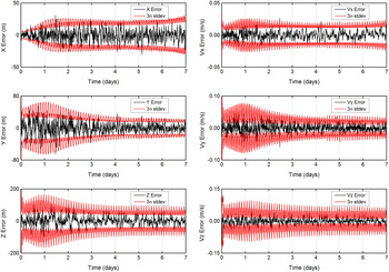
Figure 8. State estimation error for the lunar orbit phase (Halo-Halo constellation).
The computation is performed for a seven-day lunar orbit phase. The resulting RMS position error is 28·6 m and the resulting RMS velocity error is 18·9 mm/s. The probability of the position estimation error falling inside the 3σ line is 97·12%, 96·68% and 99·70%, respectively for the x, y and z components, while the probability for the velocity estimation error falling inside the 3σ line is 98·76%, 98·91%, and 99·26%, respectively for the Vx, Vy and Vz components. Besides, it can also be noticed that the z-axis position estimation error is much larger than the other two directions, and this is also due to the limited variation of observation geometry out of the xy plane. Similar simulations are conducted for the other candidate Earth-Moon L 1,2 two-satellite constellations and the final results are summarised in Table 8.
Table 8. Navigation results for the lunar orbit phase (N = 500 MC runs).

Similarly with the previous case, lunar orbit navigation performance is also related to the constellation type. The best navigation accuracy is achieved by the VL-PL constellation (ID = 8), with the average RMS position error about 20·3 m and the average RMS velocity error about 13·7 mm/s. Due to the same reason as before, Halo-Halo constellation and PL-PL constellation also present a worse performance compared with other constellations. Therefore, we can come to the conclusion that by selecting a proper combination of LPOs, the Earth-Moon L 1,2 two-satellite constellation is feasible for cislunar navigation.
5. CONCLUSIONS
This paper presents a detailed analysis of the simplified constellation architecture for the libration point satellite navigation system. As the main focus of this study, the Earth-Moon L 1,2 two-satellite constellations are proved to be feasible for continuous lunar orbit coverage. With the use of a polynomial fitting method, amplitude constraints for the feasible two-satellite constellations are approximated by quadratic polynomials. In order to evaluate the navigation performance of the simplified architecture, cislunar navigation simulations are performed for the candidate Earth-Moon L 1,2 two-satellite constellations. The final results indicate that the simplified system is available for cislunar navigation and the best accuracy of a few tens of metres can be achieved by the specific constellation configurations.
Due to the independent and extended navigation capability, the libration point satellite navigation system may play an important role in the future. The stability and station-keeping strategies for the navigation constellation will be investigated in succeeding work.
ACKNOWLEDGMENTS
This work was carried out with financial support from the National Basic Research Program 973 of China (2013CB834103) and the Research and Innovation Project for College Graduates of Jiangsu Province (KYZZ15_0035).


