1. INTRODUCTION
When a surface vessel is sailing in a seaway, waves which cause external forces and moments play an important role in its manoeuvring characteristics. These external forces and moments usually induce six degree of freedom (DOF) motions that affect the capacity of surface vessels to achieve their missions and may cause cargo damage. Therefore, some devices need to be applied to maintain vessel stability and orientation. A ship's autopilot system is used to ensure a ship navigates on the desired course by manipulating the rudder angle (Fang and Luo, Reference Fang and Luo2005). Major contributions to the development of practical steering systems were made by the Sperry Gyroscope Company. The first automatic ship steering mechanism was constructed in 1911, and a detailed theoretical analysis of a Proportional Integral Derivative (PID) controller for ship steering was presented by Nicholas Minorsky in 1922, where the yaw angle of the vessel was measured by a gyrocompass (Fossen, Reference Fossen2011; Roberts, Reference Roberts2008).
Ocean going vessel steering autopilots are designed to implement course keeping and course changing manoeuvres in the open sea (Burns, Reference Burns1995; Tzeng, Reference Tzeng1999). The classical PID controller with fixed gain is a conventional steering controller and it can give a good performance for particular operating conditions, such as track keeping control, rudder/fin roll stabilisation and heading control with an identified model (Fang and Luo, Reference Fang and Luo2006; Fang et al., Reference Fang, Lin and Wang2012; Banazadeth and Ghorbani, 2013). Some other linear controllers have also been applied to autopilot control systems, such as the internal model controller and the model predictive controller (Saari and Djemai, Reference Saari and Djemai2012; Liu et al., Reference Liu, Sun and Zou2015). Li and Sun (Reference Li and Sun2012) addressed a disturbance compensating model predictive heading controller to satisfy the state constraints.
One of the major issues in modern ship control systems is to guarantee robust stability and performance under uncertain environment disturbances and linear controllers cannot always achieve this. Several types of nonlinear controllers have been proposed to overcome the nonlinear steering problem in recent literature, such as feedback linearization, Sliding Mode Control (SMC) and an adaptive method. The typical state feedback linearization and input output linearization methods have been adopted in autopilot control systems (Moreira et al., Reference Moreira, Fossen and Soares2007; Borkowski, Reference Borkowski2014; Perera and Soares, Reference Perera and Soares2013). Zhang and Zhang (Reference Zhang and Zhang2016) introduced a sine function nonlinear feedback controller for surface ship heading control. The nonlinear state or parameters in ship steering dynamics are often linearized around specific points in these controllers and always deal with known bounded disturbances. Sliding mode control is based on the Lyapunov stability theorem and a large number of papers are available on ship control. For surface vessels, Zhang et al. (Reference Zhang, Chen and Sun2000) discussed the path following control problem in restricted waters. Alfaro-Cid et al. (Reference Alfardo-Cid, McGookin, Murray-Smith and Fossen2005) developed two decoupled sliding mode controllers for ship navigation and propulsion. Fang and Luo (Reference Fang and Luo2007) compared two sliding mode controllers for roll reduction and a track keeping control system. Harl and Balakrishnan (Reference Harl and Balakrishnan2012) considered a second order sliding mode control strategy for path following. Perera and Soares (Reference Perera and Soares2012) proposed a pre-filtered sliding mode control law to solve the nonlinear steering dynamic problem (that is, parameter uncertainties and un-modelled dynamics).
Ship dynamics can be influenced significantly due to sailing conditions and unpredictable environmental disturbances, which may affect the efficiency of crews, the accuracy of electrical mechanisms and reduce the abilities of vessels to perform their missions. Therefore, a nonlinear controller that overcomes unknown bounded external disturbances and guarantees robustness is needed. An adaptive method can be a good method to deal with these uncertainties. In the area of surface vessels, a robust adaptive controller based on Lyapunov's direct method was proposed to estimate the values of ship unknown parameters and cope with the bounded time varying terms of environmental disturbances (Do and Pan, Reference Do and Pan2006). An adaptive Neural Network (NN) method was developed to counter the unknown information of the hydrodynamic structure (Zhang et al., Reference Zhang, Zhang and Zheng2015; Shojaei, Reference Shojaei2015). The adaptive technique was also combined with Dynamic Surface Control (DSC), fuzzy and backstepping methods (Peng et al., Reference Peng, Wang, Chen, Hu and Lan2013; Li et al., Reference Li, Liu, Hilton and Liu2013; Lin et al., Reference Lin, Hsueh and Chen2014). In the area of underwater vehicle tracking control, Do (Reference Do2015) introduced a robust adaptive controller for an Omnidirectional Intelligent Navigator (ODIN) tracking under stochastic environmental loads and Liu et al. (Reference Liu, Liu and Wang2016) considered an adaptive fuzzy NN controller for an Unmanned Underwater Vehicle (UUV) that was subjected to unknown disturbances and dynamic uncertainties. Another method to reject the unknown bounded disturbance is called a disturbance observer. The observer method is always combined with a nonlinear controller for a ship motion control system, such as the backstepping method and the sliding mode controller (Liu et al., Reference Liu, Sui, Xiao and Zhou.2011; Xu et al., Reference Xu, Sun, Du and Hu2016). Lei and Guo (Reference Lei and Guo2015) proposed an extended observer to estimate the total disturbances of the ship steering system. A disturbance observer was employed with the dynamic surface control technique for a ship dynamic positioning system by Du et al. (Reference Du, Hu, Krstic and Sun2016). Still aiming at the track following and course keeping problems, to overcome the uncertain environmental disturbances under sensorless conditions, Qin et al. (Reference Qin, Lin, Sun and Yang2016) developed a sliding mode controller with a high gain observer for an underactuated ship. These studies are limited to surface vessel course keeping control under the assumption that the forward speed is constant.
Ships that proceed at certain speeds in open sea usually encounter large motions and rates due to ocean disturbances. In addition, the water resistance is increased by added resistance which may cause speed reduction and energy loss (Prpic-Orsic and Faltinsen, Reference Prpic-Orsic and Faltinsen2012). A study suggests that the magnitude of the added resistance is in the range 10%-30% of the resistance in still water (Arribas, Reference Arribas2007). From a commercial standpoint, fuel efficiency and energy conservation are being driven by business requirements in the marine industry (Armstrong, Reference Armstrong2013). In the area of ship motion control, Liu and Jin (Reference Liu and Jin2013) have done some work on the relationship of rolling and added resistance and have also provided a practical PID method to design an optimal added resistance fin control system. Subsequently, Liu et al. (Reference Liu, Jin, Grimble and Katebi2014) proposed a double Nonlinear Generalised Minimum Variance (NGMV) anti-roll control system to try to reduce the speed reduction. Yaw motion due to steering can also lead to added resistance in calm water as well as in waves. Grimble and Katebi (Reference Grimble and Katebi1986) extended a Linear Quadratic Gaussian (LQG) controller to minimise energy reduction and added resistance induced by steering in ship course keeping control. Miloh and Pachter (Reference Miloh and Pachter1989) also considered this kind of speed loss in a ship collision avoidance control system. Kim et al. (Reference Kim, Kim, Kang, Lee, Lee and Jung2015) studied the variation of ship's speed under different rudder controllers and results show that a ship's speed in regular waves may be improved by decreasing the rudder rotation velocity. Liu et al. (Reference Liu, Jin, Grimble and Katebi2016) combined both the added resistance in waves and calm water and suggested a Rudder Roll Stabilisation (RRS) control system with forward speed loss minimisation. In all these studies, the design of the control system was made under the condition of the ship moving with a certain constant speed and ship dynamics were not changed by the speed. In reality, the changes in the ship model parameters when sailing in open seas are mostly due to changes in the ship speed. The forward speed is time-varying because of the speed loss which may lead to the vessel dynamics and control parameters changing. The purpose of this paper is to design a ship autopilot control system with forward speed maintenance, considering unknown stochastic wave disturbances and parameter uncertainties caused by ship speed reduction.
The rest of this paper is organised as follows. Section 2 describes the ship dynamics and the added resistance. Section 3 presents the system structure and controller design. Simulation results and the performance of the proposed control system are discussed in Section 4. Conclusions are drawn in Section 5.
2. PROBLEM FORMULATION
The study of ship motion is very complex because a set of parameters need to be determined in the motion dynamics. In this section, the mathematical models for the ship dynamics are presented using a modification of the experimental results developed by Perez (Reference Perez2005).
2.1. Sway-yaw dynamics
The mathematical model for ship dynamics is introduced for a naval vessel. The dynamic equations of motion and corresponding forces in the body fixed frame can be represented as:
 $$\eqalign{( m-Y_{\dot {v}} ) \dot {v}+( mx_G -Y_{\dot {r}} ) \dot {r} &= Y_{\vert U \vert v} \vert U \vert v+Y_{Ur} Ur+Y_{v\vert v \vert } v\vert v \vert \cr & \quad +Y_{v\vert r \vert } v\vert r \vert +Y_{r\vert v \vert } r\vert v \vert -mUr+Y_c} $$
 $$\eqalign{( mx_G -N_{\dot {v}} ) \dot {v}+( I_{zz} -N_{\dot {r}} ) \dot {r} &= N_{\vert U \vert v} \vert U \vert v+N_{\vert U \vert r} \vert U \vert r+N_{r\vert r \vert } r\vert r \vert \cr & \quad +N_{r\vert v \vert } r\vert v \vert -mx_G Ur\hbox{+}N_c} $$
 $${\dot {\psi }} = r $$
where m is the ship mass and I zz is inertia. x G are the coordinates of the centre of gravity with respect to the body fixed frame. Sway velocity is represented by v. Yaw and its angular velocity are denoted by ψ and r, respectively. Y and N are external forces with respect to sway and yaw. Subscript c denotes the force or moment produced by the control surface.
The rudder is the device used for heading control here. The rudder induced forces and moments can be expressed in the following:
 $$Y_c =\displaystyle{{1}\over{2}}\rho A_R C_L U^2 $$
 $$N_c =-\displaystyle{{1}\over{2}}\rho A_R C_L U^2LCG $$
where ρ is the water density, A R is the area of the rudder, C L is the lift coefficient which varies with the effective angle of attack and LCG is the distance from the centre of gravity to the rudder stock.
2.2. Steering model
The ship steering system in this study is an underactuated system where the sway motion cannot be directly controlled. The study aims to achieve ship course keeping, so only yaw motion is considered. Combining the rudder action N c = N δδ and the wave disturbance, the steering dynamics can be treated as:
 $$( I_{zz} -N_{\dot {r}} ) \dot {r}=N_{\vert U \vert r} \vert U \vert r+N_{r\vert r \vert } r\vert r \vert -mx_G Ur+N_{\delta} \delta +d_w $$
where δ is rudder angle and d w is the yaw moment caused by waves.
In practice, the dynamics of the ship and actuator are changed by the time varying speed which causes parameter uncertainties. The upper bounds of disturbance and parameter uncertainties are often difficult to find. The uncertainties in a system are assumed to meet the matching conditions. In this section, a modified control model is presented, considering the time varying speed U(t) = U 0 + Δ U due to the speed loss, where U 0 is the nominal (designed) speed and Δ U is the time varying speed loss which is unknown but bounded. The steering model is written as:
 $$\dot {r}=a_1 ( U) r+a_2 r\vert r \vert +a_3 \delta +a_4 d_w $$
where  $a_{1} ( U) =\displaystyle{{N_{\vert U \vert r} \vert U \vert -mx_{G} Ur}\over{I_{zz} -N_{\dot {r}}}}$,
  $a_{2} =\displaystyle{{N_{r\vert r \vert }}\over{I_{zz} -N_{\dot {r}}}}$,
  $a_{3} =\displaystyle{{N_{\delta}}\over{I_{zz} -N_{\dot {r}}}}$,
  $a_{4} =\displaystyle{{1}\over{I_{zz}-N_{\dot {r}}}}$
Considering the dynamic uncertainties caused by the speed loss, the steering model is revised as:
 $$\dot {r}=a_1 ( U_0 ) r+a_2 r\vert r \vert +a_3 \delta +d $$
where d = d 1 + d 2 = a 1 (Δ U) r + a 4 d w is the lumped uncertainties, d 1 is the internal disturbance and d 2 is the external disturbance.
Assumption 1: The position and rate measurements of the yaw motion of the vehicle are available for feedback. The gyroscopic compass measures ψ and the yaw rate gyro measures r.
Assumption 2: The disturbance signal satisfies |d(t)| ≤ d max and d max is an unknown positive constant.
Remark 1: The sway motion cannot be directly controlled, but it is influenced by the yaw motion control commanded rudder angle.
2.3. Wave model
Complex sea states are considered to be the superposition of an infinite number of monochromatic waves, distributed in all directions. In order to simulate random waves, an International Towing Tank Conference (ITTC) long-crest wave spectrum is adopted to recreate a fully developed sea environment. The equation of wave Power Spectral Density (PSD) is given as follows:
 $$S( {\omega_i } ) =\displaystyle{{173H_{1/3}}\over{T^4\omega_i^5}}\exp \left({-\displaystyle{{691}\over{T^4\omega_i^4}}} \right)$$
where H 1/3 is the significant wave height, T is the wave period and ω i is the wave frequency of the i-th regular wave component.
In this paper, 60 regular wave components are used to form an irregular wave. The amplitude of each regular wave component ζ i and the resultant wave ζ can be obtained by the following equations:
 $$\zeta _i = \sqrt {2S( {\omega_i}) \Delta \omega} $$
 $$\zeta = \sum\limits_{i=1}^{60} {\zeta_i \cos ( {\omega_{i}t+\varepsilon_i}) } $$
where ε i is the random phase angle of the i − th regular wave, which ranges from 0 to 2π. In this calculation, the resultant wave ζ is used to calculate the external forces. This calculation is performed using code prepared in MATLAB, along with the calculation of the wave excitation forces and moments.
Generally, when a vessel is sailing with a constant speed, the wave frequency is modified as the encounter frequency and it is expressed as follows:
 $$\omega _{ei} =\omega _i -\displaystyle{{\omega _i^2 }\over{g}}\cos \beta $$
where β is the encounter angle, g is the gravitational acceleration.
In order to simulate the time series of external disturbances accurately, the time domain model of the yaw moment caused by waves is derived with the strip theory (Bhattacharyya, Reference Bhattacharyya1978) and it is given as follows:
 $$d_w =\sum\limits_{i=1}^n {[ d_{i1} \zeta _i \cos ( \omega _{ei} t+\varepsilon_i ) +d_{i2} \zeta _i \sin ( \omega _{ei} t+\varepsilon_i ) ] } $$
where  $d_{i1} =2\rho g\sum\limits_{j=1}^{N} {\lcub \exp ( -{k_{i} T_{j}}/2) T_{j} x_{j} \sin [ k_{i} B_{j} \sin ( \beta/2) ] \cos ( k_{i} x_{j} \cos \beta ) \Delta x\rcub } $, ρ is the water density, and
  $d_{i2} =2\rho g\sum\limits_{j=1}^{N} {\lcub \exp ( {-k_{i} T_{j}} /2) T_{j} x_{i} \sin [ k_{i} B_{j} \sin ( \beta/2) ] \sin ( k_{i} x_{i} \cos \beta ) \Delta x\rcub }$. ζ i and k i are the wave amplitude and the wave number of the wave component i. N and Δ x are the section number of the ship and the length of each section. T j, B j and x j are draft, breadth and the coordinate point of the section j, respectively.
2.4. Added resistance
Generally, the design of propulsive power of a ship is based on still water resistance, which will be a constant when sailing on the open sea. The forward speed will be reduced due to the added resistance which is independent of the calm water resistance. In the following we consider the added resistance caused by ship motions both in waves and in still water.
In oblique waves, the force and moment which should be applied externally can be separated according to energy considerations. The force along the x-axis (added resistance) expends energy, whereas the one along the y-axis (drift force) does not expend energy. These forces are calculated by the method proposed by Loukakis and Sclavounos (Reference Loukakis and Sclavounos1978). As shown in Figure 1, the ship is moving forward along a fixed direction. The waves arrive at an encounter angle β with a speed of propagation c. The horizontal force R T can be resolved into two components, the added resistance R x and the drift force R y.

Figure 1. Definition of added resistance and drift force.
According to the extended radiated energy theory (Loukakis and Sclavounos, Reference Loukakis and Sclavounos1978), the work of the added resistance is assumed to equate to the energy contained in the dumping waves radiated away from the ship during each wave period. The work of the horizontal force to the energy per encounter period radiated away from from the ship which moves with five degrees of freedom can be equated with strip theory approximations. Therefore, the work transformed to the fluid can therefore be expressed as:
 $$P=( -R_T ) ( -c-U\cos \beta ) T_e $$
where T e is the encounter period.
Since the purpose of this study is the control of underactuated vessels, the general Six Degree of Freedom (6-DOF) motions can be reduced to the motion in sway and yaw (that is, horizontal motions) under the assumption that the only available control input is rudder angle. For the energy radiated from the ship sideways, we obtain the energy radiated by the horizontal motions:
 $$P_{26} =\displaystyle{{\pi }\over{\omega _e }}\vint_L {b_{26} \vert {U_{RY} } \vert ^2\hbox{d}x} $$
where ω e is the encounter frequency, L is the ship length and b 26 is the motion damping coefficient. U RY is the transverse relative velocity of each ship section. Hence, the formulae to calculate the added resistance and drift force in oblique waves are:
 $$( -R_T ) ( -c-U\cos \beta ) T_e =P_{26} $$
 $$\vert {R_x } \vert =\vert {R_T \cos \beta } \vert $$
 $$\vert {R_y } \vert =\vert {R_T \sin \beta } \vert $$
where P 26 is the energy radiated by sway-yaw motion during one encounter period.
In the calm water case, when the ship travels with a yaw angle, it will create a pressure difference between the port and starboard of the ship and lead to an extra resistance, which gives a contribution to the longitudinal response of the ship. The longitudinal component of Newton's second law in the body fixed coordinate system is:
 $$M( {\dot u}-vr) =X_{\dot u} {\dot u}-R_T ( u) +( 1-\tau) T( u\comma \; n) +X_{vv} v^2+X_{vr} vr+X_{rr} r^2+X_{\delta \delta } \delta ^2 $$
where  $X_{\dot u} $, X vv,… are used to express longitudinal hydrodynamic forces on the hull and the rudder. R T (u) is the ship calm resistance, τ is the thrust deduction coefficient, T(u, n) is the propeller revolutions per second and δ denotes the rudder angle.
The main cause of resistance increase in a turning motion is due to the terms Mvr and X vr vr. Both R T (u) and T(u, n) are independent of the steering motion. The terms X vv and X rr are defined to be zero if the ship is symmetrical according to potential flow theory. The term X δ δδ 2 is the extra drag due to rudder angle and can be neglected because of its small value.
So, the added resistance due to yawing can be simplified to the following:
 $$R_{yaw} =( M+X_{vr} ) vr $$
where M is the ship mass and this resistance will be decided by the value of sway rate and yaw angle velocity.
Assumption 3: The measurement of sway can be obtained either by using a compact 6-DOF sensor or Fibre Optic Gyroscopes (FOGs) to provide continuous and accurate measurement of 6-DOF motions (MARIN, 2014).
3. CONTROL SYSTEM
The proposed closed loop autopilot system is proposed in Figure 2. Here, ψ d is the predetermined heading angle and the other desired values are set to zero. d w represents the ocean environment disturbance and the structure of the steering machine is presented in Figure 3 which presents the relationship between the commanded rudder angle and the presented rudder angle. This block diagram is a simplified hydraulic machinery model and the characteristics of this model are important since they can induce constraints on the control action, including magnitude saturation (that is, the rudder angle is constrained by the maximum angle δ max ) and rate saturation (that is, the rudder rate is limited by a maximum value  $\dot {\delta }_{\max}$).

Figure 2. Autopilot control system.

Figure 3. Steering machine model.
The sliding mode control used here is a particular type of variable structure control that can accommodate system uncertainties and it can also reject external bounded disturbances as well as quantifying the modelling and performance trade-off. Liu et al. (Reference Liu, Liu and Wang2016) adopted the SMC method to design a RRS control system with forward speed minimisation which assumed U in the ship model was a constant design speed. However, the actual forward speed varies with the speed loss in the time domain which can cause uncertainties in the dynamics of ship and actuator, which then decreases the robustness of the SMC. To improve the performance of the controller when the speed is varying over time, the following sections present the design process of two controllers.
3.1. Adaptive sliding mode controller
Considering Equation (8), the nonlinear steering system contains a nonlinear term; the feedback linearization method is adopted to convert the nonlinear part. By defining a new control signal u, the rudder angle order can be treated as follows:
 $$\delta _c =\displaystyle{{1}\over{a_3}}( u-a_2 r\vert r \vert ) $$
Then the nonlinear steering system is expressed in a linear equation:
 $$\dot {r}=a_1 ( U_0 ) r+u+d $$
The state space format is:
 $$\dot{{\bf x}}={\bf Ax}+{\bf B}u+d $$
where  ${\bf x}=\left[\matrix{ r \cr \psi}\right]$,
  ${\bf A}=\left[\matrix{ {a_{1} } &0 \cr 1 &0}\right]$,
  ${\bf B}=\left[\matrix{ 1 \cr 0}\right]$.
Let the reference state be xd = [0, ψ d] and  $\dot {{\bf x}}_{{\rm d}} =0$. A sliding manifold is used to obtain the control law and is defined as:
 $$s={\bf h}^{\rm T}{\bf x}_{{\rm e}} ={\bf h}^{\rm T}( {\bf x}-{\bf x}_{{\rm d}}) $$
where h = [h 1, h 2] T is a right eigenvector of Ac (i.e.  ${\bf A}_{{\rm c}}^{\rm T} {\bf h}=\lambda {\bf h}) $. The weighting vector h is selected by computing the equation
  ${\bf A}_{{\rm c}}^{\rm T} {\bf h}=0$ for λ = 0 (Healey and Lienard, Reference Healey and Lienard1993).
In the SMC system, a feedback control law is written as:
 $$u=-{\bf kx}+u_0 $$
where the first item of the controller is a state feedback control law (that is, an equivalent controller), the second term is a nonlinear switching control law.
Substituting Equation (25) into Equation (23), we obtain:
 $$\dot {{\bf x}}={\bf A}_{{\rm c}} {\bf x}\hbox{+}{\bf B}u_0 +d $$
where Ac = A − BkT is the combined state matrix, k = [k, 0] T is the feedback gain vector and the zero gain in k represents the integration in the yaw angle channel.
The nonlinear switching control law to reject the disturbance is chosen as follows:
 $$u_0 =-( {\bf h}^{\rm T}{\bf B}) ^{-1}[ {\bf h}^{\rm T}\hat {d}+\eta \hbox{sgn}( s) ] $$
where  ${\hat d}$ is the estimate of d.
Differentiating the sliding surface function, then:
 $$\dot {s}={\bf h}^{\rm T}{\bf A}_{{\rm c}} {\bf x}+{\bf h}^{\rm T}{\bf B}u_0 +{\bf h}^{\rm T}d-{\bf h}^{\rm T}\dot {{\bf x}}_{{\rm d}} =\lambda {\bf x}^{\rm T}{\bf h}-\eta \hbox{sgn}( s) +{\bf h}^{\rm T}\Delta d=-\eta \hbox{sgn}( s) +{\bf h}^{\rm T}\Delta d $$
where λ xTh = 0 if h is a right eigenvector, and  ${\bf h}^{\rm T}\dot {{\bf x}}_{{\rm d}} =0$ because the reference signal xd is a constant vector. The parameter
  $\Delta d=d-\hat {d}$ is the estimation error.
Since the disturbance is unknown, a better guess for it is  ${\hat d}=0$. Hence, the nonlinear switching control law becomes:
 $$u_0 =-( {\bf h}^{\rm T}{\bf B}) ^{-1}\eta \hbox{sgn}( s) $$
where η > d max‖h‖.
Equation (29) leads to the sliding mode controller:
 $$\delta _c =\displaystyle{{1}\over{a_3}}[ -kr-\displaystyle{{1}\over{h_1}}\eta \hbox{sgn}( s/\varphi) -a_2 r\vert r \vert ] $$
In this controller, a larger switching gain η corresponds to a shorter time to reach s = 0 and the system robustness against the environmental disturbance is proven. However, the upper bound of disturbance is often difficult to find in practice. So, the adaptive method is adopted to tune the controller gain without knowledge about the disturbance. Still considering the estimate of the disturbance is zero, the robust switching control law of the total controller is modified as:
 $$u_0 =-( {\bf h}^{\rm T}{\bf B}) ^{-1}\hat {\eta }\hbox{sgn}( s) $$
where  ${\hat \eta}$ is the estimate of the adjustable gain and is a positive value.
The adaptation law is written as:
 $$\dot {\hat {\eta }}=\displaystyle{{1}\over{\alpha}}\vert s \vert $$
where α > 0 is the adaptation gain.
Then the differentiation of the sliding surface is:
 $$\dot {s}={\bf h}^{\rm T}( \dot {{\bf x}}\hbox{-}\dot {{\bf x}}_{{\rm d}} ) ={\bf h}^{\rm T}( {\bf A}_{{\rm c}} {\bf x}+{\bf B}u_0 +d) ={\bf h}^{\rm T}{\bf B}u_0 +{\bf h}^{\rm T}d=-\hat {\eta }\hbox{sgn}( s) +{\bf h}^{\rm T}d $$
Selecting the Lyapunov function,
 $$V=\displaystyle{{1}\over{2}}s^2+\displaystyle{{1}\over{2}}\alpha \tilde {\eta }^2 $$
where  $\tilde {\eta }=\hat {\eta }-\eta $ is the estimation error.
 $$\eqalign{\dot {V}&=\displaystyle{{1}\over{2}}s\dot {s}+\displaystyle{{1}\over{2}}\alpha \tilde {\eta }^2=s[ {\bf h}^{\rm T}d-\hat {\eta }\hbox{sgn}( s) ] +\alpha ( \hat {\eta }-\eta ) \dot {\hat {\eta }} \cr & = s{\bf h}^{\rm T}d-\hat {\eta }\vert s \vert +( \hat {\eta }-\eta ) \vert s \vert =s{\bf h}^{\rm T}d-\eta \vert s \vert \le 0} $$
 Equation (35) holds for all time for the external disturbance. The parameter  ${\hat \eta}$ chosen in Equation (31) implies that the system trajectory will move and reach the sliding surface in a finite time and the sliding surface declines to zero, so the control law given by Equation (25) guarantees the sliding mode sustained (Huang et al., Reference Huang, Kuo and Chang2013). The tanh function has replaced the signum function to attenuate the chattering effect. Hence, the Adaptive Sliding Mode Controller (A-SMC) is:
 $$\delta _c =\displaystyle{{1}\over{a_3}}[ -kr-\displaystyle{{1}\over{h_1 }}\hat {\eta }\tanh ( s/\varphi ) -a_2 r\vert r \vert ] $$
where φ is the boundary layer thickness.
3.2. Nonlinear disturbance observer
In the last section, the estimate of disturbance is treated as zero because no knowledge of the disturbance can be available. An alternative method to process this problem is called a Disturbance Observer (DO). Since the yaw acceleration is not easy to obtain, it is also difficult to construct the acceleration signal from yaw rate by differentiation. So, a modified observer called a Nonlinear Disturbance Observer (NDO) is adopted here (Chen, Reference Chen2004; Yang et al., Reference Yang, Li and Yu2013).
Define a variable:
 $$z=\hat {d}-p( r\comma \; \psi ) $$
Let the function p(r, ψ) be given by the following equation:
 $$\displaystyle{{\hbox{d}p}\over{\hbox{d}t}}=\displaystyle{{L( r\comma \; \psi ) }\over{a_4 }\dot {r}} $$
Define the observer error signal:
 $$\tilde {d}=d-\hat {d} $$
According to the linear disturbance observer, a DO is proposed as:
 $$\eqalign{\dot {\hat {d}} & =L( r\comma \; \psi ) ( d-\hat {d}) =L( r\comma \; \psi ) ( \dot {r}-a_1 ( U_0 ) r-a_2 r\vert r \vert -a_3 \delta ) -L( r\comma \; \psi ) \hat {d} \cr & = L( r\comma \; \psi ) ( \dot {r}-a_1 ( U_0 ) r-a_2 r\vert r \vert -a_3 \delta ) -L( r\comma \; \psi ) [ z+p( r\comma \; \psi ) ] \cr &=-L( r\comma \; \psi ) z+L( r\comma \; \psi ) [ \dot {r}-a_1 ( U_0 ) r-a_2 r\vert r \vert -a_3 \delta -p( r\comma \; \psi ) ] } $$
In general, prior information about the derivative of the disturbance is unavailable, and the disturbance varies slowly relative to the observer dynamics. Then it reasonable to suppose that:
 $$\dot {d}=0 $$
Hence, the derivative of the observer error is:
 $$\dot {\tilde {d}}=\dot {d}-\dot {\hat {d}}=-\dot {\hat {d}}=-L( r\comma \; \psi) \tilde {d} $$
Let the functions in Equation (36) be chosen as:
 $$L( r\comma \; \psi ) =a $$
where a is a positive constant.
Then the following equations are obtained:
 $$p( r\comma \; \psi ) = ar $$
 $$\displaystyle{{\hbox{d}p}\over{\hbox{d}t}} = a\dot {r} $$
Combining the above equations, the update law can be written as:
 $$\eqalign{\dot {z} & =\dot {\hat {d}}-\displaystyle{{\hbox{d}p}\over{\hbox{d}t}}=\dot {\hat {d}}-L( r\comma \; \psi ) \dot {r} \cr &=-L( r\comma \; \psi ) z+L( r\comma \; \psi ) [ -a_1 ( U_0 ) r-a_2 r\vert r \vert -a_3 \delta -p( r\comma \; \psi ) ] \cr &=-az+a\lcub -[ a+a_1 ( U_0 ) ] r-a_2 r\vert r \vert -a_3 \delta \rcub } $$
Hence, the NDO is given by:
 $$\hat {d}=z+ar $$
The nonlinear switching control law in this SMC is defined as:
 $$u_0 =-( {\bf h}^{\rm T}{\bf B}) ^{-1}[ {\bf h}^{\rm T}\hat {d}+\eta _0 \hbox{ sgn}( s) ] $$
The differentiation of the sliding surface is:
 $$\dot {s}={\bf h}^{\rm T}{\bf A}_{{\rm c}} {\bf x}-\eta _0 \hbox{ sgn}( s) +{\bf h}^{\rm T}d-{\bf h}^{\rm T}\hat {d}={\bf h}^{\rm T}{\bf A}_{{\rm c}} {\bf x}-\eta _0 \hbox{ sgn}( s) +{\bf h}^{\rm T}\tilde {d}=-\eta _0 \hbox{ sgn}( s) +{\bf h}^{\rm T}\tilde {d} $$
Let the Lyapunov function be chosen as:
 $$V=\displaystyle{{1}\over{2}}s^2+\displaystyle{{1}\over{2a}}\tilde {d}^2 $$
Differentiation of the Lyapunov function with respect to the trajectory of states gives:
 $$\dot {V}=s\dot {s}+\displaystyle{{1}\over{a}}\tilde {d}\dot {\tilde {d}}=-\eta _0 \hbox{ sgn}( s) +{\bf h}^{\rm T}\tilde {d}s-a\tilde {d}^2\le 0 $$
where the gain must satisfy  $\eta _{0} \gt \Vert {\bf h} \Vert \cdot \Vert {\tilde {d}} \Vert $.
Hence, the final output of the sliding mode controller with nonlinear disturbance observer (NDO-SMC) is written as:
 $$\eqalign{\delta _c & =\displaystyle{{1}\over{a_3}}[ -kr-\hat {d}-\displaystyle{{1}\over{h_1}}\eta_0 \tanh ( s/\varphi ) -a_2 r\vert r \vert ] \cr & = \displaystyle{{1}\over{a_3}}[ -kr-\displaystyle{{1}\over{h_1}}\eta _0 \tanh ( s/\varphi ) -a_2 r\vert r \vert ] -\displaystyle{{1}\over{a_3}}\hat {d}} $$
where the first term in Equation (52) can be treated as a sliding mode controller that rejects the disturbance  ${\tilde d}$. A diagram of this control system is shown in Figure 4.

Figure 4. Modified autopilot control system.
4. SIMULATION RESULTS
A heading control system simulation of a naval vessel is demonstrated (Perez, Reference Perez2005). The nominal ship speed is 15 knots and it is assumed to be sailing in a sea environment that is infinitely deep. The wave disturbance is simulated with a significant wave height of 2 m and an average period of 7·5 s. In order to avoid the effect of stall angle the magnitude constraint for the rudder angle of δ max = δ stall = 25° and the vessel is equipped with two rudders. The maximum rudder rate is  $\dot {\delta }_{\max } = 15\, ^{\circ} /s$. The desired state trajectory is assumed to be xd = (0, 0)T, the initial state vector is x = (0, 0)T, the initial guess of η is 2 for the SMC. The initial values of the adaptation law are set as η (0) = 2 and η 0 (0) = 1 ·5. The boundary layer is chosen as φ = 1. The linear state feedback gain is k = 0·1 and (η min, η max) is considered as (1, 10). The nonlinear disturbance observer parameter is selected as a = 20. The vessel sails in an oblique wave condition with an encounter angle of 135° and the time domain simulation is done by a fourth order Runge-Kutta (Fossen, Reference Fossen2011) numerical integration method with the time step of 0·1 s.
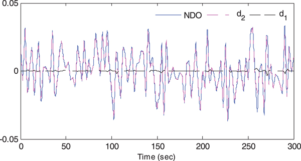
The computation simulations of a course keeping manoeuvre of a nonlinear ship autopilot system are presented in Figures 5 to 10, and the corresponding simulation values (Root Mean Square (RMS) value) are presented in Table 1. Figure 5 shows the time series of wave height sand yaw moments which represent the external disturbance. Figure 6 presents non-dimensional results of the proposed observer, where d 1 is the internal disturbance (that is, the system uncertainties caused by the speed loss) and d 2 is the external disturbance (the yaw moment caused by waves). A better NDO performance can be obtained when a larger value of L(r, ψ) is chosen, since an overlarge value can cause an algebraic loop problem in the process of numerical calculation, the value (a = 20) used in this study is reasonable.
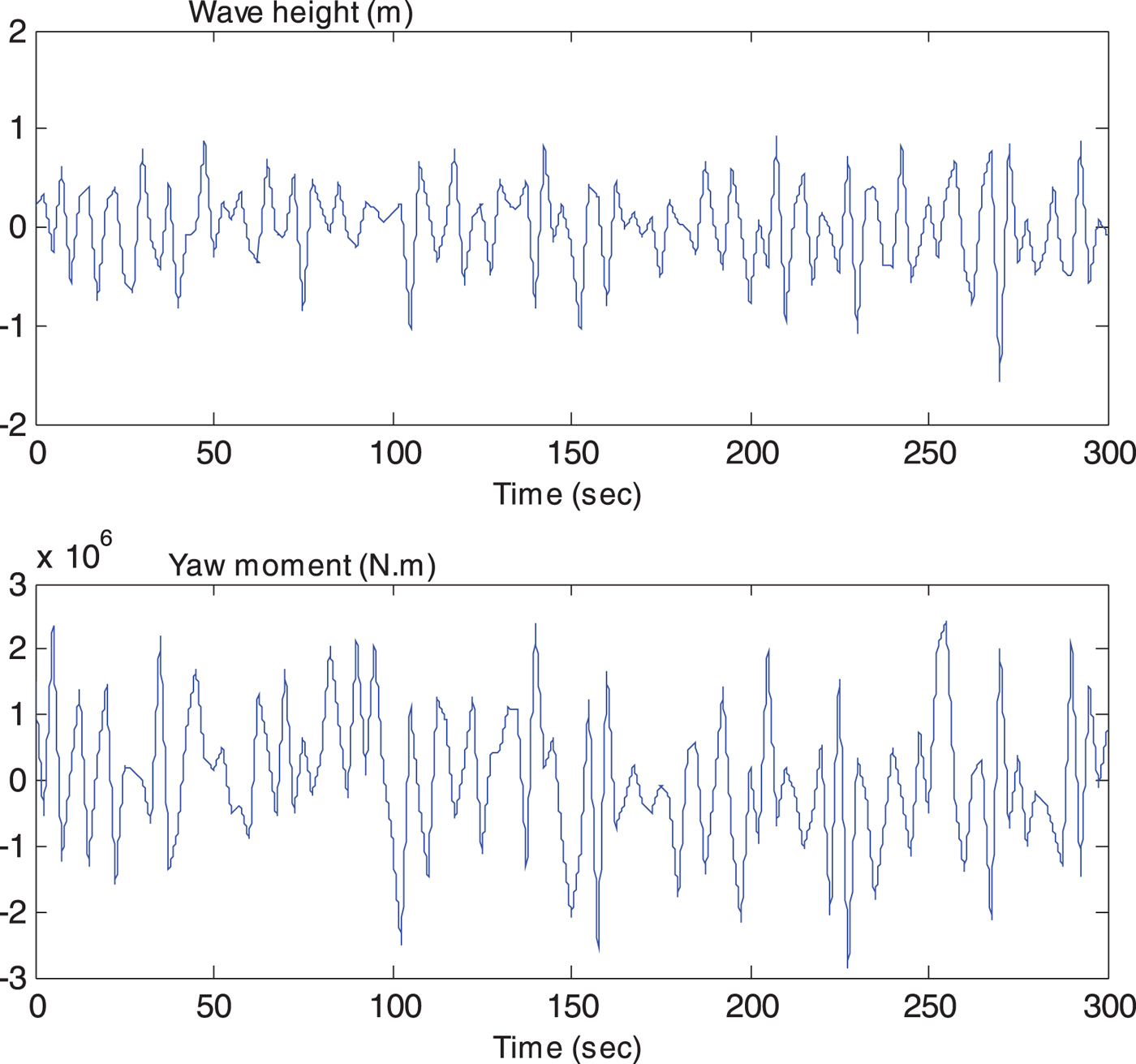
Figure 5. Time series of wave height and yaw moment.
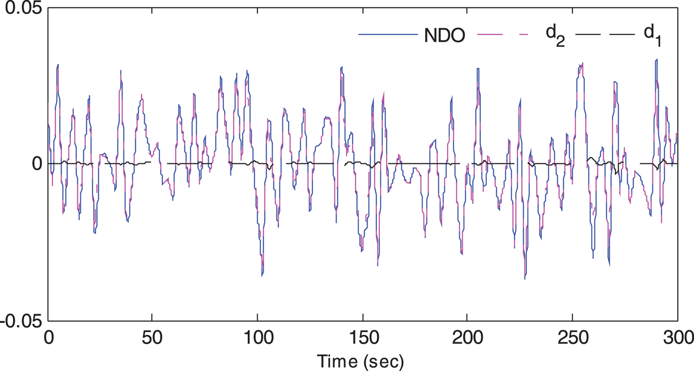
Figure 6. Simulation results of the disturbance observer.
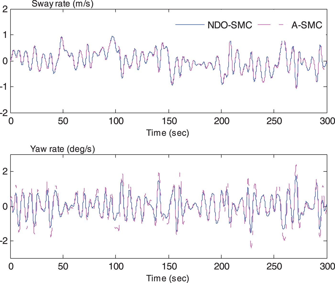
Figure 7. The comparison of sway rate and yaw rate.
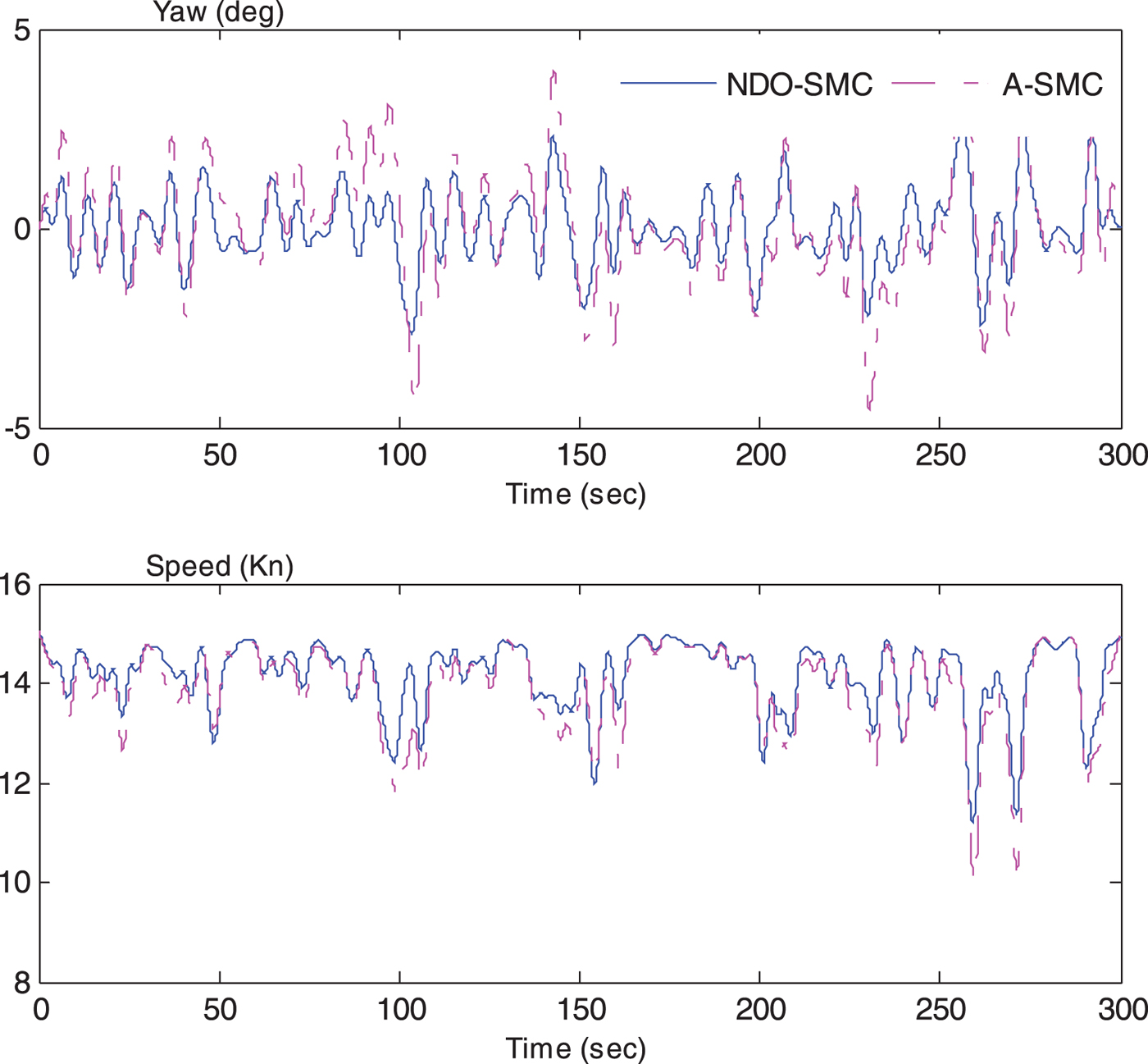
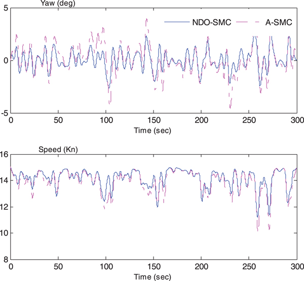
Figure 8. The comparison of yaw angle and speed.
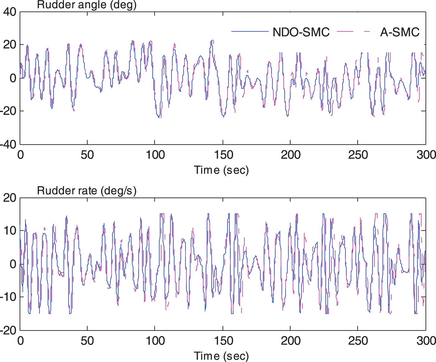
Figure 9. The comparison of rudder angle and rate.
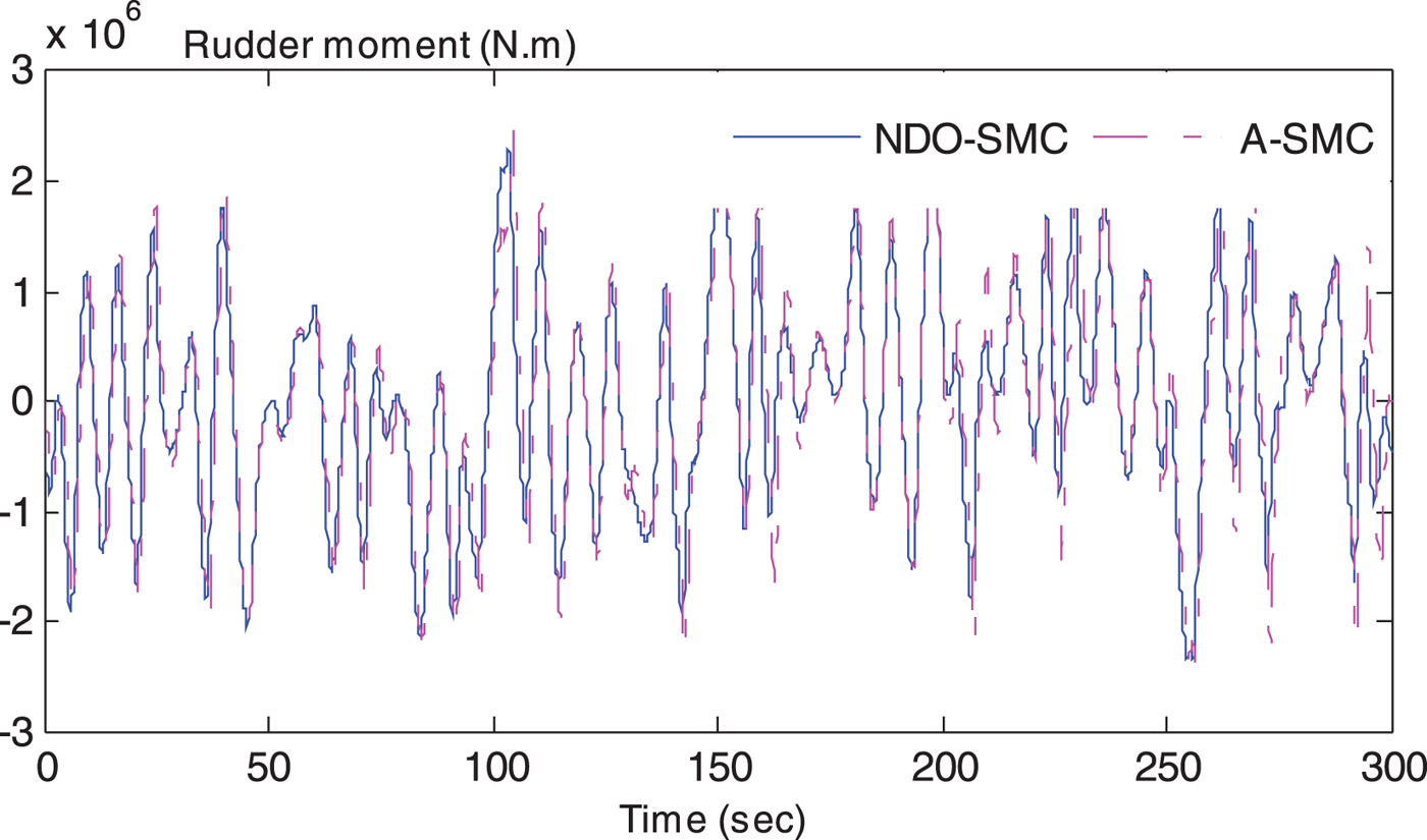
Figure 10. The comparison of rudder moment.
Table 1. Cost values of simulation

Figure 7 shows the simulation of sway rate and yaw rate which could induce added resistance in both waves and calm water according to Equations (13) and (18). The dashed lines represent the time series of the adaptive sliding mode controller while the solid lines mean the time response of the sliding mode controller with NDO. The NDO-SMC can achieve smaller values of sway velocity and yaw rate, see Table 1 (0·38 and 0·59, respectively). That is to say, the added resistance due to sway–yaw coupling motion in waves and the added resistance by yawing motion in calm water have declined, compared with the A-SMC method. Hence, the NDO-SMC method can maintain the forward speed more effectively, as shown in Figure 8, and the mean value of the forward speed can be raised by 0·25 knots as against the A-SMC method which cannot be ignored in a real voyage of a vessel. Figure 8 also presents the heading control performance; the yaw response is significantly improved by the proposed NDO-SMC algorithm.
Figure 9 presents a comparison of rudder commands. The A-SMC method causes larger amplitudes of rudder angle and rudder rate; the additional rudder command may cost more energy to drive actuators and cause rudder angle and rate saturation, which may enhance the mechanical wear and tear of actuators. This is also the reason why a saturation element is needed. The values calculated from the cost function are listed in Table 1. Thus, the A-SMC scheme can produce a greater rudder moment to reject the wave moment because of the larger rudder angle, as shown in Figure 10, but it does not achieve a better sailing performance. The reason maybe that the NDO can estimate the disturbance more accurately and then the controller can give more suitable rudder commands to match the yaw moment.
5. CONCLUSION
Considering forward speed keeping, this paper has discussed two sliding mode controllers to deal with the total unknown bounded disturbance for a nonlinear vessel steering control system, based on an adaptive controller and the nonlinear disturbance observer method. As presented in the simulation results, all controllers have successfully converged the ship actual course into the reference course and maintained the ship speed effectively, especially the proposed NDO-SMC scheme. As noted in the simulations, the rudder response can approach the limitation of rudder angle and rudder rate due to the control output signals requirement. The vessel autopilot system performance is evaluated under a trade-off between the rudder control gain and a faster course keeping response. Comparing the control performance, the ship heading response under the nonlinear observer method represents the superior performance that requires lower rudder actuations and better heading response.