


1. Introduction
An aircraft wing can carry a high-resolution aerial remote sensing system imaging load (such as array synthetic aperture radar, array SAR) in addition to its original function. The high-precision estimation of wing deformation error according to the measured data of sensors, such as high-precision position and orientation system (POS) and fibre Bragg grating (FBG) strain sensor, is an important method to measure the position and orientation of imaging load nodes and the length of interference baseline between nodes with high accuracy. Recently, mechanism modelling and stochastic theory modelling has enabled its implementation.
Mechanism modelling is used to find and establish a mathematical relationship between the mechanism of flexure and its internal and external factors, and then compensate the amount of flexure based on the relationship (Girhammar and Atashipour, Reference Girhammar and Atashipour2015; Zohreh and Hamidreza, Reference Zohreh and Hamidreza2017; Zhang et al., Reference Zhang, Nie and Cai2019). The relationship between the deflection angle and the specific force measured by the inertial navigation network is established to realize the correlation between the deflection angle and the inertial navigation measurement (Kelley and Carlson, Reference Kelley and Carlson1994). The deflection is estimated according to the linear function of the specific force and is calculated based on the given specific force data (Pehlivanoglu and Ercan, Reference Pehlivanoglu and Ercan2013). These two methods introduce the relationship between specific force and flexural deformation in the modelling process, which, however, must rely on extensive repeated test data to establish the relationship between deflection and related physical quantities. Therefore, it is quite complicated to find the relationship between the internal and external mechanisms causing the flexural deformation, of which the mechanism modelling is based on many less-universal simplifications and assumptions. Furthermore, the effectiveness of this method must be further verified.
Schneider first applied the second-order Markov model to the transfer alignment technology between two inertial sensor assemblies (ISAs) installed in different positions on nonrigid structures (Schneider, Reference Schneider1983). Since then, scholars have been assuming that the wing deformation caused by air disturbance is a Gauss Markov stochastic process (Lu et al., Reference Lu, Fang, Liu, Gong and Wang2017; Gong and Chen, Reference Gong and Chen2019; Mohammed et al., Reference Mohammed, Wail and Frank2020), which is based on the Markov model (Wu et al., Reference Wu, Chen and Qin2013; Geng et al., Reference Geng, Wu and Xu2018) or AR model (Dong et al., Reference Dong, Li and Lai2010) to establish the estimation model of deflection. Kain (Kain and Cloutier, Reference Kain and Cloutier1989) analysed the aircraft wing vibration data by fast Fourier transformation (FFT), and finally found a third-order Markov model by post-processing and fitting the flight data. Based on Kain's method, Spalding (Spalding, Reference Spalding1992) decomposed the flexure motion of the wing into two states: quasi-static flexure and high-frequency flexure. The former is the low-frequency wing flexure caused by the dynamic state of the aircraft or the sudden change of the aircraft load, and the latter is a 5–10 Hz wing structure vibration caused by the internal and external disturbance of the aircraft. Both are considered to be the third-order Markov model. Jan et al. (Reference Jan, Jürgen and Gert2004) also proposed the deflection as a third-order Markov model, who estimated the model parameters based on the deflection data obtained from the first-order difference of the inertial device measurement data.
At present, scholars regard the deflection of the wing as a second- or third-order Markov model, which only involves algorithm simulation, model parameters and orders, exclusive of the actual data. This paper proposes a new method of wing deformation modelling to separate and identify the influence of multiple disturbance sources. Aiming at the limitation that the wing deformation between the traditional primary and secondary inertial navigation system (INS) is only affected by a single disturbance and based on the empirical parameter modelling, this paper probes the separation of internal and external disturbance based on the real-time observation of sensors, and the wing deformation classification modelling carried out based on that parameter identification.
In Section 2, the impact of external disturbance is analysed in detail, and the impact of internal disturbance is proposed in Section 3. Section 4 introduces the method of extracting and separating the deflection data of wing. Section 5 presents the proposed method based on AR model parameter identification, and Section 6 provides a detailed demonstration of the AR model of wing deformation combined with the real flight data under the influence of engine vibration and turbulence disturbance. Finally, Section 6 presents the conclusions.
2. Influence of external disturbance on wing deflection
With a high-resolution aerial earth observation system, its active space is mainly located in the troposphere of the atmosphere (0 km ~ 11 km) (Soren et al., Reference Soren, Jan and Howard1995; Lou, Reference Lou2002; Gonzalez et al., Reference Gonzalez, Bachmann, Scheiber, Andres and Krieger2008), and the external disturbance of the aircraft is mainly carrier manoeuvre and air disturbance. During the imaging period, the main concern of the aircraft comes to be air disturbance since no manoeuvre has been carried out. The air disturbance includes discrete gust and continuous gust, the former representing the deterministic change of wind speed and the latter showing itself as a kind of atmospheric turbulence. The wind speed profile is a random function with continuous change of wave shape and frequency over time (Etkin, Reference Etkin2012; Akin and Kahveci, Reference Akin and Kahveci2019; Grillo and Montano, Reference Grillo and Montano2019). Therefore, it will generate certain or random additional aerodynamic forces, which will make the wings of the aircraft do up and down in rigid motion and local elastic vibration. Thus, the external disturbance focuses on atmospheric turbulence.
The atmospheric turbulence model mainly includes the engineering simulation method and numerical simulation method. The engineering simulation method is mainly based on the Dryden and Von Karman model (Mouyon et al., Reference Mouyon, Imbert and Montseny2002; Ji et al., Reference Ji, Chen and Li2017) established by the Monte Carlo method, which is mainly used in the construction of the real-time flight environment simulation platform of the carrier aircraft and the aircraft control platform based on MATLAB Simulink. It is not able to simulate or analyse the impact of atmospheric turbulence on the deflection deformation of the wing. The numerical simulation method is to simulate the flow of atmospheric turbulence based on computational fluid dynamics (CFD). Combined with computational structural mechanics (CSM), it can carry out fluid structure coupling calculation to realize the response simulation of wing structure under the influence of atmospheric turbulence.
2.1 Wing model
The simulation wing adopts a standard Boeing 103 airfoil derived from profile software, and the structure is shown in Figure 1. The wing chord is 0⋅6 m, with a total length of 3 m; the skin thickness is 2 mm, with the skeleton structure being composed of wing beam, wing rib and truss strip; the wing material is aluminium alloy 7075. To compare the wing deformation under different flight conditions (speed and height) in the follow-up study, the first measuring point is 0⋅1 m away from the root of the left end, and the rest are set every 0⋅2 m. A total of 15 measuring points are set, from left to right, and the measuring point numbers are 1,2,…,15°.

Figure 1. Wing structure model
2.2 Simulation of wing flow field
The software Integrated Computer Engineering and Manufacturing code for Computational Fluid Dynamics (ICEM CFD) is used to build the simulation wind tunnel test field, as shown in Figure 2, which mainly includes turbulent inlet and outlet areas, wall area and wing structure. The turbulence entrance and exit areas are mainly used to set the corresponding physical quantities of the carrier's flight conditions to simulate different flight conditions of the carrier. The Spalart–Allmaras turbulence model suitable for wing flow is adopted. The gas is set to constant, and the atmospheric density of different heights is determined according to Table 1; the specific parameters are determined according to Table 1 with the working speed of the current carrier, the pressure and temperature values at the height set by the physical quantity at the inlet, and the pressure and temperature values set by the physical quantity at the outlet. In the ANSYS static structural module, the left end of the simulation wing is set to fix support end, and the right end is the cantilever state of the free end; the fluent module is used to simulate the aerodynamic load applied to the wing, to compute the wing structure deformation.
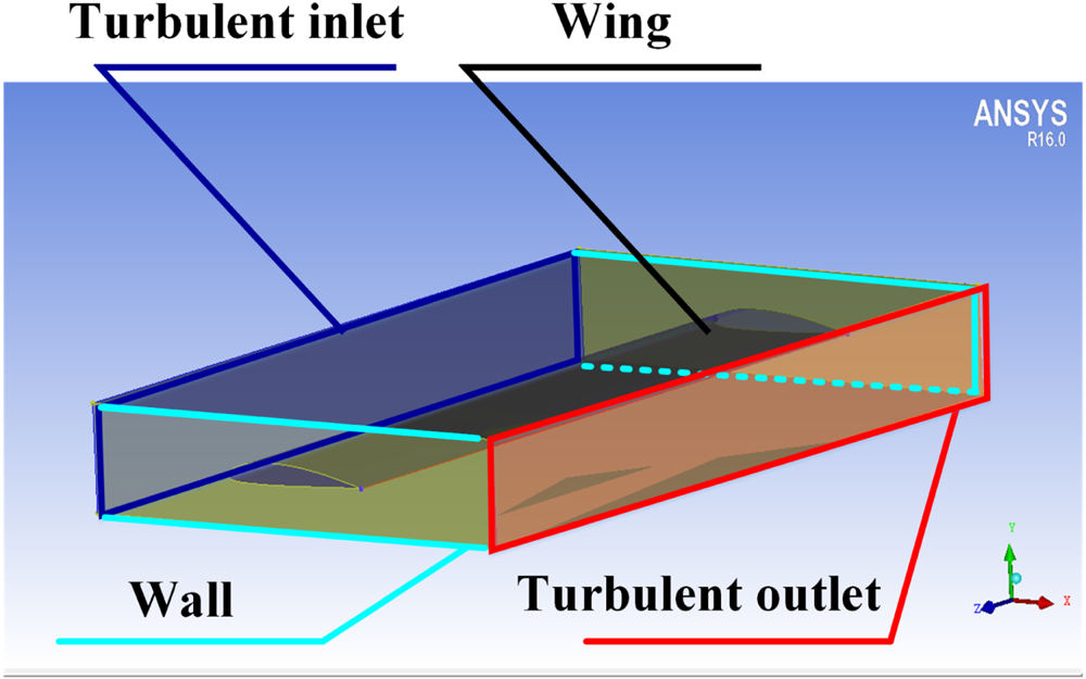
Figure 2. Wing flow field area
Table 1. Physical parameters of different flight altitude (GJB, 5601-2006)

2.3 Atmospheric turbulence influence on the wing deflection
Taking the aircraft to ground observation system working at 3 km height and 200 m/s as an example, the aerodynamic load and turbulence velocity change felt by the wing skin in Figure 1 are calculated by using ANSYS fluent module, and the results are shown in Figure 3. The yellow line in Figure 3 shows the change of turbulence velocity when the turbulence flows through the wing (left legend, unit: m/s), and the blue, green, yellow areas on the surface show the aerodynamic load on the wing (right legend, unit: Pa); and the static structural module is used to calculate the deformation of the wing under the aerodynamic load (unit: m), as shown in Figure 4. It shows that the change of wing structure surface from the left end to the right indicates the increase of wing deformation.

Figure 3. Load on wing and change of turbulent velocity

Figure 4. Lateral displacement of wing structure
The flight altitude remains unchanged; in other words, the atmospheric pressure and temperature are not changed, and only the change of the carrier's working speed affects the atmospheric turbulence, with the effect of atmospheric turbulence changing from 150 m/s every 5 m/s to 250 m/s on the wing deformation being simulated, as shown in Figure 5. Where, the x-axis represents the flight speed, the y-axis represents the different positions of the wing, and the z-axis represents the lateral and axial deformation.
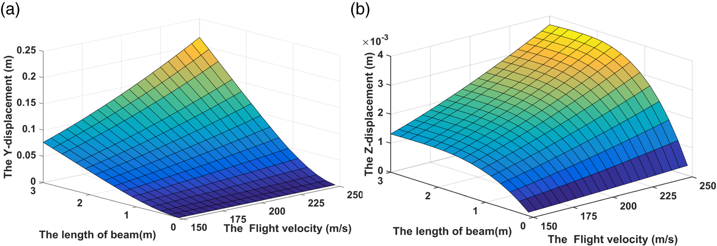
Figure 5. Wing deformation of aircraft at different working speeds. (a) Transverse deformation. (b) Axial deformation
To analyse the influence of turbulence change caused by working height change on wing deformation, wing deformation data must be collected, involving the simulation carrier working height changing from 2⋅5 km to 6 km every 0⋅5 km and working speed changing from 125 m/s to 300 m/s every 25 m/s. Here, only the deformation of measuring point 15 is listed, and the carrier working height is represented by the height pressure, as shown in Figure 6; where, the x-axis represents the atmospheric pressure of the aircraft at different working heights (increase in altitude, decrease in atmospheric pressure), the y-axis represents different working speeds, and the z-axis represents wing deformation.

Figure 6. Wing deformation of test point 15 under different working conditions. (a) Transverse deformation. (b) Axial deformation
In Figures 5 and 6, influence of the carrier's working speed and the atmospheric turbulence caused by the height change on the wing deformation is quite significant. To determine the relationship between the reactions, Table 2 lists the relation between height change and deformation caused by the working speed of 300 m/s, and Table 3 lists the relationship between different speeds and the corresponding deformation at an attitude of 3 km.
Table 2. Relationship between height and wing deformation

Table 3. Relationship between velocity and wing deformation

The data in Tables 2 and 3 show a high correlation, with the correlation coefficient both between height and speed of the carrier, and between the lateral deformation and axial deformation of the wing close to 1. Therefore, the height and speed parameters can be selected to build the mapping relationship between atmospheric turbulence and the deflection deformation of the wing.
3. Influence of internal disturbance on wing deflection
3.1 Characteristic analysis of engine vibration
The internal disturbance of aircraft is mainly the plastic deformation of the wing and the vibration of the engine. Plastic deformation can be used as an initial quantity to be eliminated or suppressed through ground calibration, which will not be involved here. The main cause of the engine vibration is the rotor imbalance (Bonello and Hai, Reference Bonello and Hai2009; Tavakolpour et al., Reference Tavakolpour, Nasib and Sepasyan2015; Yu et al., Reference Yu, Zhang, Ma and Hong2018) with certain inherent characteristics. Now it is assumed that the y-axis direction of the coordinate system established by the engine rotor is the same as the y-axis of the wing coordinate system in Figure 4, and the expression of unbalanced excitation force can be given as

In formula (1), e = unbalance, ${\theta _e}$ = unbalance phase, ${\omega _F}$
 = rotor speed and m = rotor mass.
The allowable residual unbalance represents the maximum unbalance of the engine, which is a standard calculation quantity, and its expression is

In formula (2), m = mass of rotor and ${e_{\textrm{per}}}$ = allowable residual unbalance, which is usually expressed in g mm/kg.
It can be seen from literature (GB/T, 9239.1-2006/ISO, 1940-1:2003) that the balance level of aero engine rotor is G6.3, and the relationship between the working speed, and the allowable residual unbalance is shown in Table 4.
Table 4. Relationship between ${\omega _F}$ and ${e_{\textrm{per}}}$

In Table 4, as the engine speed increases gradually, the allowable residual unbalance degree decreases accordingly, that is, the tolerance degree for the factor of aero engine rotor unbalance decreases, so it is particularly important to analyse the influence of engine vibration on wing deformation at high speed.
3.2 Influence of engine vibration on wing deflection
In Figure 1, the total weight of the wing structure is 78 kg. According to statistics (Compiled by the general editorial board of aircraft design manual, 1999), the mass of the power system is 185⋅25 kg, and the mass of the engine is 179⋅85 kg (turbojet engine). Using the mass of the engine to replace the mass of the rotor approximately, the specific values of allowable residual unbalance and unbalanced force corresponding to the high-pressure rotor at different speeds can be calculated as shown in Table 5.
Table 5. The relationship between the working speed of rotor and the allowable unbalance and unbalanced force

Since the change of phase does not affect the magnitude of amplitude, the phase angle is ${0^0}$ and the calculated speed is 10,000 r/min, the corresponding unbalanced force is

In Figure 7, the unbalanced force changing from 0 to 0⋅2 s is listed. It is a high-frequency sinusoidal disturbance on the wing, which can be reflected by the wing vibration acceleration.

Figure 7. Unbalanced force at 10,000 r/ min
With the help of the transient structural module of ANSYS, the unbalanced force disturbance is applied to the simulated wing structure in Figure 1. The installation point is set 0⋅75 m from the root to load the force, and the acquisition frequency of 200 Hz is set to obtain the wing vibration acceleration information. Table 6 lists the wing vibration acceleration and frequency information under different engine rotation speeds (the positive direction of the y-axis is specified as the positive direction of acceleration).
Table 6. Wing flutter at different engine speeds

In Table 6, the correlation coefficient between different engine speeds and the acceleration value of wing vibration deformation is close to 1, showing a highly correlated relationship. However, the original output information of POS equipment contains the acceleration process, so the acceleration information measured by POS is selected to reflect the change of wing deformation caused by engine vibration.
4. Extraction and separation of wing deflection
In the aerial remote sensing system, the influence of the internal and external disturbance on the wing deflection exists simultaneously, while the influence mechanism is different. In the simulation experiment in Section 2, the mapping relationship between the external disturbance (atmospheric turbulence) and the wing deformation is constructed with parameters of altitude and velocity. For the simulation experiment in Section 3, the mapping relationship between the internal disturbance (engine vibration) and the wing deformation is constructed with acceleration. In this section, based on the actual flight experiment, through the height, velocity and acceleration parameters, the internal and external interferences on the wing are separated, and the wing deflection under the internal and external interference is extracted.
In an experiment, the main and the sub POS systems are installed as shown in Figure 8. The main POS is installed on the belly and the sub POS is installed on the wing. The flight path of the aircraft carrier is shown in Figure 9, in which the red part is the imaging working section. The angular velocity data output by the POS of the imaging section is shown in Figure 10. Among them, Fig. (a) is the angular velocity data in the x-direction, Fig. (b) is the angular velocity data in the y-direction, and Fig. (c) is the angular velocity data in the z-direction. Red represents the angular velocity information output by the main POS, and blue represents the angular velocity information output by the sub POS.

Figure 8. Distributed POS flight experiment system

Figure 9. Actual flight path

Figure 10. Angular velocity information output by POS. (a) X-axial angular velocity. (b) Y-axial angular velocity. (c) Z-axial angular velocity
Suppose that the expression of angular velocity signal ${\omega _{ib}}$ output by sub POS is
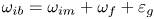
In formula (4), ${\omega _{im}}$ = angular motion information of the aircraft body provided by the main POS; ${\omega _f}$
 = angular motion between the main sub nodes, that is, the angular velocity of the deflection effect of the aircraft wing; and ${\varepsilon _g}$
 = drift of the sub POS gyroscope and represents the fixed and random errors of the gyroscope measurement. The formula describes the quantitative relationship between the angular velocity measurement information provided by the main and the sub POS and the wing deflection angle.
4.1 Elimination of ɛg influence based on FIR filter
Firstly, FFT transformation is carried out based on the static measurement data of POS equipment to determine the noise amount of the gyroscope, as shown in Figure 11, the spectrum distribution of gyroscope measurement in the x, y, and z directions in turn.

Figure 11. Spectrum distribution of gyro measurement under static condition
Then, FFT transform is applied to the gyroscope measurement of the sub POS in the flight experiment in Figure 9, and the result is shown in Figure 12, which illustrates the spectrum distribution of the measurement of the gyroscope in the x, y, and z directions in turn.
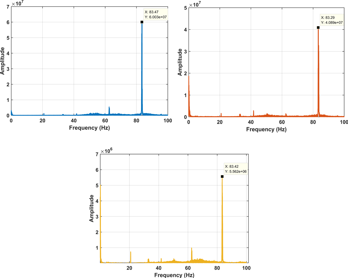
Figure 12. Spectrum distribution of gyro measurement under dynamic condition
Comparing Figure 11 with Figure 12, based on the characteristics of the main/sub POS measurement data, the cut-off frequency of the finite impulse response (FIR) low-pass filter is 83⋅3 Hz, and the filter length is determined by the Hanning window. Figure 13 shows the raw signal (blue) and FIR filter processed signal (red) quality of the sub POS.

Figure 13. Signal quality before and after y-direction angular velocity filtering
It can be seen from Figure 13 that after FIR filter processing, the ${\varepsilon _g}$ effect is well eliminated.
4.2 Extraction of deflection based on first-order difference
The measurement of the x-axis, y-axis and z-axis of the gyroscope indicates the angular velocity changes of the carrier along the pitch, roll and heading, respectively. The deflection deformation of the wing between the main and the sub POS is generally the largest in the y-axis direction (i.e. roll direction) and has the greatest impact on the wing. Therefore, the deformation along the y-axis is mainly considered. Here, the first-order difference processing is performed on the filtered roll angle velocity signal to preliminarily extract the deflection of the wing, as shown in Figure 14.

Figure 14. Deflection of wing between main and sub nodes
After the influence of ${\varepsilon _g}$ is removed, the relative angular velocity of the primary and secondary nodes is the angular velocity of the wing deflection. Processing the difference between two consecutive sampling time points of POS measurement data

Realisation of information acquisition of vehicle flexure movement $\partial {\omega _f}$ . In the calculation, the initial value of deflection under the action of gravity under the initial static condition is not considered temporarily, and the initial deflection information ${\omega _f}$
 can be obtained after superposition calculation according to the continuous time point.
4.3 Separation of internal and external disturbances
Empirical mode decomposition (EMD) assumes that all complex signals composed of intrinsic mode functions (IMFs) have different bandwidths and reflect the local frequency characteristics of the signal. Therefore, based on its characteristics, the original signal is decomposed by frequency, and a set of n basic IMF sequences from low frequency to high frequency and a residual trend signal r are obtained. The expression is

Through empirical mode decomposition, the extracted angular velocity ${\omega _f}$ can obtain a limited IMF sequence from low frequency to high frequency, which has a certain degree of self-adaptability reflected in the empirical mode decomposition based on POS measurement data. For the measurement data in different flight segments, the IMF sequence is a set of basic functions with both frequency and amplitude changes. Finally, with the help of the correlation between IMF sequence and POS measurement data, the wing deformation under the influence of atmospheric turbulence and engine vibration is extracted. Besides, the correlation between orientation and velocity in POS and the IMF sequence reflect the influence of atmospheric turbulence on the wing deflection, and the influence of engine vibration on the wing deflection is shown according to the acceleration information correlation.
The wing deflection between the main POS and the sub POS is extracted, and the modal decomposition is carried out. Finally, 15 groups of IMF values are obtained, as shown in Figure 15. According to the correlation of different frequency IMF sequences with altitude, velocity and acceleration, a specific IMF sequence is selected to calculate the wing deflection under the influence of internal and external disturbances. Table 7 lists the correlation between wing deflection and altitude, and velocity and acceleration extracted for distributed POS flight data.

Figure 15. IMF series of wing deflection between main and sub POS
Table 7. Correlation between deflection and physical parameters of wing

From Table 7, it can be seen that the relationship between IMF component, height and velocity (i.e. the larger correlation of turbulence) is mainly reflected in the low-frequency segment, such as IMF11-IMF15; the relationship between IMF component and acceleration (i.e. the larger correlation of engine vibration) is mainly demonstrated in the high-frequency segment, such as IMF1-IMF3. In addition, the wing deformation under the two effects can be separated for the superposition calculation of specific IMF sequence, as shown in Figure 16.

Figure 16. Angular velocity of wing deflection between main and sub POS. (a) Engine vibration effects. (b) Atmospheric turbulence effects
5. Modelling research based on AR model parameter identification
Based on the FIR filter, first-order difference processing and empirical mode decomposition, the angular velocity of wing deflection effect under the influence of internal and external disturbances can be extracted and separated, and the wing deformation modelling can be carried out accordingly. There are two main methods of wing deformation modelling: deformation mechanism modelling and stochastic theory modelling. The former is to find the internal mechanism by analysing the cause and effect of the tested object, which is not universal. The latter is mainly based on the identification model parameters research, such as the AR model and moving average (MA) model of AR, with numerous data to represent the deformation law and state of the wing, using statistical methods to establish a model with good fit with the original data, which has strong online correction ability. In this study, the second- and third-order Markov model based on empirical parameter setting of wing deformation modelling is transformed into the modelling research based on the AR model parameter identification of POS measurement data, to improve the reliability of deformation modelling.
AR (P) model is

In Equation (7), p is the model order, which represents the influence of the first p data on the current data; $({{\phi_1}, {\phi_2}, \cdots , {\phi_p},{\varepsilon_g}} )$ is the model parameter; and ${\varepsilon _j}$
 is the Gaussian white noise volume, ${\hat{\varepsilon }_j}\sim ({0c{\sigma^2}} )$
 . The Akaike information criterion (AIC) test criterion (Arnold, Reference Arnold2010; Loannidis, Reference Loannidis2011) is used to determine the order p and the least square method to obtain the model parameters. The mean square error (MSE) value is used to evaluate the accuracy of the model to fit the original data.
The AIC criterion is used to determine the order of the model, to let the formula $\textrm{AIC}(n) = {N_d}\ln {\sigma ^2} + 2{n_d}$ reach the minimum value, where m is the data quantity, p is the order of the model and σ2 is the variance value of the built model. Using the least square estimation model parameters, for the sample sequence $\{{{x_t}} \}$
 , when $m \ge p$
 the estimation of the white noise is ${\hat{\varepsilon }_m} = {x_m} - ({{{\hat{\phi }}_1}{x_{m - 1}} + {{\hat{\phi }}_2}{x_{m - 2}} + \cdots + {{\hat{\phi }}_p}{x_{m - p}}} )$
 , ${\hat{\varepsilon }_j}\sim ({0,{\sigma^2}} )$
 , the estimation of the autoregressive coefficient ${\phi _1},{\phi _2}, \ldots ,{\phi _p}$
 in the AR (P) model will be the case when the sum of the squared residuals ${\sum\nolimits_{m = p + 1}^N {[{{x_m} - ({{{\hat{\phi }}_1}{x_{m - 1}} + {{\hat{\phi }}_2}{x_{m - 2}} + \cdots + {{\hat{\phi }}_p}{x_{m - p}}} )} ]} ^2}$
 reaches the minimum value.
For

$Y = X\phi + \varepsilon$ can be obtained, so the function of the sum of the squares of the residuals is expressed as

Equation (8) is derived from parameter $\phi$

Make Equation (9) to 0 to calculate the least square estimation of $\varphi$ as
as

Use the least square estimation of error variance as

According to these calculation steps, a third-order AR model ${x_t} = {\phi _1}{x_{t - 1}}\textrm{ + }{\phi _2}{x_{t - 2}}\textrm{ + } \cdots \textrm{ + }{\phi _p}{x_{t - p}} + {\varepsilon _g}$ is initially set up with MATLAB and a section of random data is generated. The initial value is set to ${\omega _1}\textrm{ = }{\omega _2}\textrm{ = }{\omega _3}\textrm{ = }0$
 . The model parameters of this segment of data are identified by the least square estimation, and the results are shown in Table 8.
Table 8. AR model identification parameter results

It can be seen from Table 8 that these methods can be used to realise the parameter identification of the model, and with the increase of data length, the accuracy of the model parameter identification is higher.
6. Experiment
For the modelling of the deflection between the main nodes and the sub nodes of the distributed POS system, the overall flow chart is shown in Figure 17.

Figure 17. Modelling data processing flow
For a distributed POS experimental data, extract the wing deflection data under atmospheric turbulence and engine disturbance, and determine the AR model parameters based on the change of AIC value and MSE value, as shown in Figure 18.

Figure 18. Relationship between model order, AIC value and MSE value. (a) Effect of engine vibration. (b) Effect of turbulence
For the model establishment under the influence of the engine, it can be seen from Figure 18(a) that the AIC value and MSE value of the established model decrease continuously in the process of increasing the order from the first order to the 20th order, but the changing margin is relatively lower than the 14th order. According to the calculation, the AIC values of the 13th, 14th and 15th orders are −6⋅99, −7⋅39, and −7⋅40; MSE values are 1⋅11 × 10−3, 6⋅17 × 10−4 and 6⋅14 × 10−4, respectively; the AIC values of the 100th and 200th orders are −7⋅86, −7⋅88, and MSE values are 3⋅85 × 10−4 and 3⋅74 × 10−4, respectively. In this paper, when selecting the order of the model implicating impact on wing deformation which appears to be too large for any increase in the calculation of the whole system, the real-time performance reducing the AIC value of the model with the previous order is greater than 0⋅05, and the AIC value of the model with the later order is less than 0⋅03, and the model with the AIC value and MSE value changing slowly from this order is the best fitting model.
For the model establishment under the influence of turbulence, it can be seen from Figure 18(b) that in the process of increasing the order from the first to the 20th order, the AIC value and MSE value of the established model decrease continuously, but the AIC value of the established model changes slowly from the fourth order, while the MSE value of the established model changes slowly from the second order. According to the calculation, the AIC values of the 4th-, 5th-, and 10th-order models are −42⋅90, −43⋅19 and −43⋅24, respectively, and the MSE values are 2⋅34 × 10−19, 1⋅75 × 10−19 and 1⋅66 × 10−19, respectively. In this paper, choosing the model order of turbulence effect on wing deformation is consistent with the model of engine effect on wing deformation. In other words, the AIC value of the former model is greater than 0⋅05 and the difference value of the latter model is within 0⋅03, and the key is that the model with slow change of AIC value and MSE value from this order is the best fitting model.
For wing deformation estimation, the aim is a real-time compensation scheme for distributed POS measurement data, but the post-processing algorithm only appears in the experimental stage. In this paper, with the help of the previous flight experiment data, a process of real-time parameter identification based on post-processing simulation is adopted, which is to identify the original 0~md s data and build a p-order AR model, then add the MD second data as a data package to the original data each time and carry out the model order and parameters of the original model based on AIC criterion and least square estimation method keep updating.
6.1 Parameter identification of 5s interval data
First, the p-order AR model is established by parameter identification for the data of 0-5 s. Then, starting from 5 s, the data of 5 s is added to the original data as a data sequence, and the parameters of the original p-order model are constantly modified. Figures 19–21 lists the order changes of the model, with red for turbulence effects and blue for engine effects in each illustration.

Figure 19. Modelling of disturbances in the first-round flight 5 s interval data

Figure 20. Modelling of disturbances in the second-round flight 5 s interval data

Figure 21. Modelling of disturbances in the third-round flight 5 s interval data
It can be seen from Figures 19–21 that for every 5 s of data increase, the parameters of the main and the sub POS measurement data are identified to establish that the turbulence influence wing model is kept at order 5 and the engine vibration influence wing model is kept at order 14.
6.2 Parameter identification of 10 s interval data
First, the p-order AR model is established by parameter identification for the data of 0–10 s. Then, starting from 10 s, the parameters of the original p-order model are continuously modified by adding 10 s (200 Hz, 2000 data) as a new data sequence to the original data. Figures 22–24 lists the order changes of the model. In each diagram, red represents turbulence and blue represents engine influence.

Figure 22. Modelling of disturbances in the first-round flight 10 s interval data

Figure 23. Modelling of disturbances in the second-round flight 10 s interval data

Figure 24. Modelling of disturbances in the third-round flight 10 s interval data
From Figures 22–24, we can also draw the same conclusion that data of each input of 10 s is the same as that of each input of 5 s: the turbulence influence model is a fifth-order AR model, and the engine influence model is about a 14th-order AR model.
Based on these two processing methods, according to the judgement principle that the higher the fitting degree and the lower the MSE (i.e. the closer the built model is to the original data), the parameter identification results of the wing deflection modelling based on the AR model for the sub POS data are: the turbulence influence wing deformation model is fifth-order (${\omega _t} = {A_1}{\omega _{t - 1}} + {A_2}{\omega _{t - 2}} + \cdots + {A_5}{\omega _{t - 5}} + {\varepsilon _g}$ ), while the engine influence wing deflection model is about 14th-order (${\omega _t} = {A_1}{\omega _{t - 1}} + {A_2}{\omega _{t - 2}} + \cdots + {A_{13}}{\omega _{t - 13}} + {A_{14}}{\omega _{t - 14}} + {\varepsilon _f}$
 ). In addition, the method in this paper provides experimental verification for the previous second- or third-order Markov model calculation for the impact of air disturbance, and provides a new idea for high-precision transfer alignment scheme.
7. Conclusion
High accuracy estimation of wing deformation is the key to ensuring high-resolution aerial remote sensing imaging. Mechanism modelling and stochastic theory modelling are two traditional methods, which only focus on single disturbance based on empirical parameter modelling. The external disturbances (air disturbances, etc.) and internal disturbances (engine vibration, wing structural materials, etc.) are two main factors that affect the wing deformation. Aiming at the complex multi-source disturbance of aircraft wing, this paper analyses and separates the influence of external disturbance (mainly turbulence disturbance of air) and internal disturbance (mainly engine vibration) of the wing based on the real-time observation of distributed POS measurement system, and classifies the deformation of the wing based on the parameter identification of the AR model. Combined with the real flight data in the laboratory, the wing deformation model under the influence of engine vibration is given as a 14th-order AR model, and the wing deformation model under the influence of turbulence disturbance is given as a fifth-order AR model.
Because of the excessively high-order final model, it fails to meet the real-time requirements of aerial remote sensing Earth observation system. At present, it is mainly used in the post-processing of aerial remote sensing data, and the baseline measurement accuracy is better than 3 mm, according to the deformation measurement accuracy. However, the real-time performance of the model requires further study. In addition, the influence of wing structure material is not considered in modelling. In the later stage, based on the strain measurement of FBG sensor and modal theory, the disturbance of wing structure material is separated.
Acknowledgement
This work was supported by the National Natural Science Foundation of China (grant 61873019, 61421063,61722103, 61973020, 61661136007), by Aeronautical Science Foundation of China (grant 20170551004), by Key Technologies and Methods of Airborne Distributed Measurement (grant 6140413030302).
Conflict of interest statement
None declared.


