2.1. Overview of air traffic control flow

Before the conventional calculation method is introduced, an overview of air traffic control flow under distance-based separation is given. This separation standard is applied on oceanic routes. When an aircraft flies on a certain route, it has to be separated from other aircraft vertically or horizontally by the safety margin. Here, only the longitudinal separation is considered. The applied longitudinal separation standard differs by aircraft equipment, and there are two separation standards, time-based separation and distance-based separation. The reduction of time-based separation has been studied in previous research (Mori, Reference Mori2011; Reference Mori2012) so here distance-based separation is discussed. In the NAT region, a shorter time-based separation has recently been introduced with ADS-C and Controller-Pilot Data-Link Communications (CPDLC) aircraft (NAT, 2013), but the basic concept is similar to the distance-based separation explained here.

When distance-based separation is applied, ADS-C is required. ADS-C is an on board device which sends data automatically to the air traffic controller, and is usually operated via a satellite connection. The data sent includes the current aircraft position, future predicted aircraft position, and other basic data (e.g. airspeed). There are basically two timings to send data via ADS-C. First, the aircraft sends data at a constant interval, and this data is called a periodic position report. Second, the data is sent when the aircraft passes a waypoint. Therefore, the longest interval between two position reports is the periodic position report interval, but sometimes more frequent position reports are sent. Compared to High Frequency (HF) voice communication, the ADS-C message is automatically sent, which reduces the workload of both pilots and controllers. In addition, ADS-C messages include various data that helps the controller but there is a delay in data sending, and the data sent might not be monitored in real time even if the data is sent. With these characteristics taken into account, the risk of collision is calculated.

Another condition to apply distance-based separation is that the aircraft is certified by RNP4 or RNP10. RNP4 aircraft can fly more accurately than RNP10, and this certification affects the separation standard. Consider a pair of aircraft applying distance-based separation. If both aircraft are RNP4 certified, the separation minimum is set to 30 nm, otherwise it is 50 nm. In addition to the difference of the separation standard, the periodic position report interval also differs between RNP4 aircraft and RNP10 aircraft; it is currently set to ten minutes for RNP4 aircraft and 27 minutes for RNP10 aircraft in the Fukuoka FIR. ICAO indicates the maximum periodic position report intervals for each RNP, and the Air Navigation Service Provider can determine the intervals within these ranges. According to ICAO PANS-ATM (ICAO, 2007), the maximum periodic report interval shall be 14 minutes for RNP4 aircraft and 27 minutes for RNP10 aircraft. However, based on the result of the previous safety analysis, ten minutes' periodic report interval is mandatory for RNP4 aircraft in Japan. Obviously, shorter periodic report intervals reduce the risk of collision, but frequent periodic report interval also means higher costs of data exchange, therefore aircraft operation costs increase. Therefore, the longest periodic report interval which suffices for the required maximum collision risk is desirable. In this research, only the 30 nm separation standard is considered.

2.2. Risk of collision and its calculation by conventional method

The term “sufficiently small collision risk” was mentioned in Section 1 and here the method that determines this is presented. ICAO instructs that the risk of collision is calculated quantitatively, and it should be proven that the risk of collision is less than the target level of safety (TLS). The value of TLS is also set by ICAO, and 5·0×10⁻⁹ is used for longitudinal distance-based separation. There is a common methodology to calculate the risk of collision for longitudinal distance-based separation, so it is introduced first. The basic idea of the conventional method is described in Hsu (Reference Hsu1981), Anderson and Lin (Reference Anderson and Lin1996) and the pre-implementation safety analysis is described in Fujita (Reference Fujita2008). From the next paragraph, there are many parameters defined for the calculation, and the Appendix provides a summary of parameters for easier understanding.

Firstly, the Reich collision risk model is introduced (Reich, Reference Reich1966). This model calculates the probability of mid-air collision between two aircraft in a very simple form. It assumes that an aircraft is a box, and the collision happens when two boxes overlap. This model was first used for the reduction of longitudinal separation from 15 minutes to ten minutes for the NAT track system (NATSPG, 1978). Although this model assumes steady states, i.e. the error does not change with time, this assumption holds at en-route level flight phase and this model is widely used for collision risk estimation especially on a Performance Based Navigation (PBN) flight. When the longitudinal separation is considered, the risk of collision is calculated as the product of three-dimensional risk of collision.

(1)$$N_{ax} = 2P_y (0)P_z (0)P_x \left( {\displaystyle{{v_x} \over {2\lambda _x}} + \displaystyle{{v_y} \over {2\lambda _y}} + \displaystyle{{v_z} \over {2\lambda _z}}} \right)$$

where P _x, P_y(0) and P _z(0) are the longitudinal, lateral and vertical overlap probabilities. v _x, v_y and v _z are average longitudinal, lateral, and vertical relative speeds of an aircraft pair. λ _x, λ_y and λ _z are the average aircraft length, wingspan and fuselage height, respectively. When considering longitudinal separation, P _x is a key parameter and the problem is how to calculate P _x. The other parameters can be assumed to be constant.

P _x is affected by many factors, but here two major factors are considered first, i.e. the nominal separation (x) and the controller intervention buffer time (τ). Even if minimum 30 nm separation is considered, not all aircraft apply exactly 30 nm separation, and there are many aircraft applying 31 nm, 32 nm,… separation. The longer nominal separation reduces the collision probability, so the actual situation should be considered. When separation violation happens, the controller tries to resolve the conflict. However, even if the controller notices the aircraft potential conflict, the aircraft cannot resolve the conflict in real time, so τ describes the required time to resolve conflict after the controller notices the separation violation. τ is mathematically defined as the duration from the time when the periodic report should be obtained to the time when the conflict is totally resolved by controller's and pilot's actions. Large τ means that two aircraft get closer unintentionally, and the collision probability increases. The value of τ depends on the case, and it is explained in detail in Section 3.2.3. Considering these two factors, P _x is calculated by the following expression as in Equations (4) and (5) in Fujita's work (Fujita, Reference Fujita2008).

(2)$$P_x = \sum\limits_{x,\tau} {E_x (x)E_\tau (\tau )P_x (x,\tau )} $$

where E _x(x) and E _τ(τ) are the relative frequency of the nominal separation being x and the required time to resolve conflict being τ. P _x(x,τ) is the longitudinal overlap probability when x and τ are constant. If a stationary model is assumed, P _x(x,τ) is constant, but here the time-dependent model is applied and calculated as shown in the next paragraph.

In order that a controller can assure longitudinal separation, ADS position reports and predicted position reports are used. The controller has to confirm that the minimum separation is assured between aircraft, but the position report interval is large (ten or 27 minutes) as explained in the last section, so the current separation should be calculated based on the previous position report and the prediction for the next position report, as shown in Figure 1. The black aircraft image indicates the reported position and its time, and the shadowed aircraft image indicates the future predicted position and its time. The periodic position report interval is defined as T, and the T _g is the gap of the reporting time between two aircraft. The position report is not synchronized (i.e. T _g is not usually equal to zero), so the position report is not obtained at the same time for all aircraft. Therefore, for the controller to understand the current separation, the current position is linearly interpolated between the obtained position and the predicted position, as shown by dotted lines. At each time, the red line indicates the separation between aircraft, and the controller has to assure that this separation should be greater than the required minimum separation. However, this separation is interpolated so it differs from the “actual” separation. The difference between the separation the controller notices (defined as nominal separation) and the actual separation is defined as the position prediction error, i.e. the difference between the current reported position and the predicted position estimated by the data sent before, also as shown in Figure 1. Aircraft are in conflict when the position prediction error is the same as the nominal separation. From here on, the position prediction error, not the actual separation, is considered to calculate the risk of collision.

Figure 1. Separation and position report image.

Consider two RNP4 certified aircraft flying at the same flight level and the same route. It is assumed that the position report is obtained by periodic report only, which leads to conservative risk estimation. The preceding aircraft is denoted by Aircraft 1, and the following aircraft is denoted by Aircraft 2. The following assumptions are applied to calculate the risk of collision.

1. (1) The position report also includes some error due to, for example, GPS position estimation error and the error of each aircraft is denoted by x ₁ and x ₂.

2. (2) The position prediction error of each aircraft increases linearly and its rate is v ₁ and v ₂, which are defined as speed prediction error. This speed prediction error can be obtained from the position prediction error divided by the duration between the current ADS-C message and the ADS-C message used for prediction. The duration is usually the same as T. t is the time, and t=0 is the time when Aircraft 1 obtains the latest position report. Under this condition, the position prediction error e is calculated based on the following expression as in Fujita's work (Fujita et al., Reference Fujita, Nagaoka and Amai2006; Fujita, Reference Fujita2008). Negative position prediction error indicates separation decrease.

   (3)$$e = \Delta x + \Delta X(t)$$
   (4)$$\Delta x = x_1 - x_2 $$
   (5)$$\Delta X(t) = \left\{ {\matrix{ {v_1 t - v_2 (T - T_g + t)} & {t \lt T_g} \cr {v_1 t - v_2 (t - T_g )} & {t \ges T_g} \cr}} \right.$$

Δx is the relative position prediction error coming from the initial position error and is constant with time. ΔX(t) indicates the relative position prediction error which varies with time. e is the total relative position prediction error, and it can be divided into time dependent ΔX(t) and non-time dependent Δx. Δx is composed of the initial position estimation error, which is independent of the aircraft, so the relative error is just the difference of each initial position error. As for ΔX(t), each aircraft has an independent speed prediction error, so the position prediction error varies with time. According to Smith et al. (Reference Smith, Hutton, Martin and Arnold2012), the largest risk of collision is obtained when T _g=0, and the stationary model can be applied when T _g=0. However, the time-dependent model is applied here to avoid any conservative assumptions. The relative position prediction error is calculated by the difference of position prediction error of each aircraft. However, the position report is not synchronized between the aircraft, so the position prediction error of Aircraft 2 is changed before and after the position report as described in Equation (5).

Here, f _x(e;v ₁,v ₂,t,T _g,T) is defined as the probability density function of e assuming that all five parameters are constant. When all five parameters are constant, ΔX(t) is also constant, so f _x(e;v ₁,v ₂,t,T _g,T) can be written by the following form using g ₁(x) and g ₂(x) which are the probability density functions of the initial position error of Aircraft 1 and 2. It is assumed that the initial position error is independently distributed.

(6)$$f_x (e;v_1, v_2, t,T_g, T) = (g_1 *\, g_2 )(\Delta X(t))$$

where g ₁ * g ₂ indicates the convolution of g ₁(x) and $g_2 (x )$ functions. Then, P _x(x,τ) is given by the following expression. The idea is based on Hsu's work (Hsu, Reference Hsu1981) and is extended by Anderson and Lin (Reference Anderson and Lin1996). The following expression is formed by Fujita (Reference Fujita2008):

(7)$$\eqalign{P_x (x,\tau ) =& \int_0^T {\displaystyle{{dT_g} \over T}\int_0^{T + \tau} {\displaystyle{{dt} \over {T + \tau}} \int_{ - \infty} ^\infty {\,f_v (v_1 )dv_1 \int_{ - \infty} ^\infty {\,f_v (v_2 )dv_2}}}} \cr & \times \int_{ - x - \lambda _x} ^{ - x + \lambda _x} {d(\Delta X)g_1* g_2 (\Delta X(t;v_1, v_2, T_g, T))}} $$

where f _v(v) indicates the probability density function of speed prediction error. Here, it is assumed that the speed prediction error of two aircraft is independently distributed. There are five integrals, and the last integral shows the longitudinal overlap condition where the relative position prediction error comes between −x−λ _x and −x+λ _x, as the nominal separation is x. However, ΔX(t) is a function with five parameters, and T is constant while the others are variables. Therefore, the other four parameters are distributed with a probability density function. T _g is a gap parameter and it is random between 0 and T, i.e. the probability density function is a uniform distribution. As for t, the collision can occur anytime before the conflict is resolved, i.e. the collision can happen between t=0 and t=T+τ. τ is the controller intervention buffer defined before. As for v ₁ and v ₂, the probability density function follows f _v(v).

Using the above expressions, the risk of collision can be calculated.

2.3. Parameter Description

In order to calculate the risk of collision, many parameters and probability density functions have to be set as explained in the previous chapter. However, some of the parameters do not affect the risk of collision so much, and they are determined in advance according to other documents. All parameters needing to be set are summarised in Table 1. All values set here are chosen conservatively.

Table 1. Parameters and functions required to calculate the risk of collision.

As for the probability density functions of the initial position error, this depends on the aircraft equipment. When the aircraft has GPS installed, the initial position error is small, but otherwise it is large. RNP4 aircraft usually have GPS and Japan certificates RNP4 aircraft only with GPS. However, GPS is not necessarily mandatory for RNP4 certification according to ICAO, so here it is assumed that 10% of aircraft do not have GPS installed. Under such a mixture of equipment, the final risk of collision is calculated by the following form based on Fujita (Reference Fujita2008), using the value α which indicates the ratio of aircraft installing GPS.

(8)$$N_{ax\_total} = (1 - \alpha )^2 N_{ax} (GPS,GPS) + 2\alpha (1 - \alpha )N_{ax} (GPS,nonGPS) + \alpha ^2 N_{ax} (nonGPS,nonGPS)$$

3.1. Data Acquisition and Airspace Considered

Before introducing the new calculation method, the current risk of collision is calculated based on the conventional method. This time, NOPAC (NOrth PACific) routes in Fukuoka FIR are chosen as a target airspace, as shown in Figure 2. NOPAC routes are located north east of Japan, and are the busiest oceanic routes in Fukuoka FIR. NOPAC consists of five routes, but this time, the three busiest northern routes are considered. R220 and R580 are westbound only and A590 is eastbound only. ADS-C data was obtained between April 2010 and June 2013 via the Oceanic Data Processing (ODP) system installed in Japan, and a total of 115,028 data sets are obtained. To calculate the required parameters, the following criteria are applied to isolate improper data.

• • The position report data is removed when the aircraft is changing flight level or flying below 29000 ft.

• • The position report data is removed when the aircraft deviates from the nominal path by more than 5 nm.

• • The predicted position is removed when the flight level of the predicted position is different from the reported flight level.

• • The position report data is removed when the estimated ground speed from the previous position is greater than 800 kt or less than 200 kt.

• • The predicted position is removed when the ground speed from the current position to the predicted position is greater than 800 kt or less than 200 kt.

Figure 2. NOPAC routes.

3.2. Probability density functions obtained from data

According to Table 1, three probability density functions have to be set from the data. Each function will be obtained as follows.

3.2.1. f_v(v) Probability density function of speed prediction error

Speed prediction error can be easily obtained from the data. Here, the data for which the position report interval is 27 minutes is used. To obtain the probability density function, a certain distribution function must be assumed, and here Laplace (double-exponential) distribution is used as expressed by the following equation.

(9)$$f\,(x;\mu, \lambda ) = \displaystyle{{\exp ( - |x - \mu |/\lambda )} \over {2\lambda}} $$

This distribution function is widely used in the field of safety analysis, and it is a longer-tailed distribution and provides a more conservative result than a normal distribution. The Laplace distribution has a log-linear tail, while the normal distribution has a log-quadric tail. There are two parameters in the function, and they are usually estimated based on the obtained data. When fitting probability density function, the maximum likelihood estimation is often used. Let each speed prediction error be v _i. Two parameters are optimized by maximizing the following log likelihood.

(10)$$\sum {\log (\,f\,(v_i ;\mu, \lambda ))} $$

By optimizing these parameters, μ=−2·18, λ=6·85 are obtained. Figure 3 shows the obtained data and the fitted distribution function. The figure shows that the function fits the data well, but the tail of the distribution seems to be a bit higher than that of a Laplace distribution. In order to confirm that the obtained data can be modelled by Laplace distribution, the kurtosis is obtained. The kurtosis is the value that describes the degree of tail of the distribution. A large kurtosis indicates that the distribution has a wide distribution. The kurtosis of the Laplace distribution is 3·0, while the kurtosis of the obtained data is 3·14, which means that the obtained distribution is slightly wider than the Laplace distribution. Next, it is validated whether the values of kurtosis are significantly different. It is assumed that the obtained data is based on the Laplace distribution with obtained parameters, and 56,488 data sets are picked up 1000 times. In each iteration, the kurtosis is calculated and 95% confidence interval of the kurtosis is calculated. According to the result, 95% confidence interval of the kurtosis is between 2·90 and 3·33, and the obtained kurtosis is within this range. Therefore, it is concluded that the obtained data follows the Laplace distribution, and the obtained parameters are used.

Figure 3. Relative frequency of speed prediction error.

3.2.2. E_x(x) Relative frequency of nominal separation

Relative frequency of nominal separation can also be obtained easily from the data. In each position report, the nearest preceding aircraft distance is calculated. Until the next position report, it is assumed that the obtained distance is maintained. Figure 4 shows the relative frequency of nominal separation to 200 nm where both aircraft are RNP4 certified. Although there are many aircraft which have more than 200 nm separation, it is assumed that all aircraft have less than 200 nm separation and the relative frequency is calculated, which leads to conservative risk estimation. According to the figure, separation less than 50 nm is rarely used, mainly because the number of RNP4 certified aircraft is still low. However, the ratio of aircraft RNP4 certified is gradually increasing, and there will be more chances to apply 30 nm separation in the future.

Figure 4. Duration of nominal separation for a pair of both RNP4 aircraft.

Once a new procedure is implemented, it is used for a long time. Therefore, the frequency of nominal separation should account for future traffic increase, too. In the future, it is expected that all aircraft will apply distance-based separation, not time-based separation, and all aircraft will have a certificate of RNP4, not RNP10. In addition, the traffic volume will rise to 1·5 times current levels in the next 20 years in Japan according to CARATS, the Japanese future plan (Civil Aviation Bureau, Japan, 2010). Considering this, the future traffic levels should be assumed.

However, it is difficult to estimate the future traffic, and Smith et al. (Reference Smith, Hutton, Martin and Arnold2012) propose that the nominal separation is modelled by a Gamma distribution. However, here it is estimated based on the current nominal separation data and future traffic volume of RNP4 aircraft. Figure 4 shows that the relative frequency of nominal separation increases from zero to a certain level, and it is almost flat after that. Therefore, the relative frequency of the nominal separation is assumed to be modelled by the following equation:

(11)$$E_{x\_future} (x) = \left\{ {\matrix{ 0 \cr {y_0 (x - x_0 )/x_1 - x_0 \quad} \cr {y_0} \cr} \matrix{ {x \lt x_0} \cr {x_0 \les x \lt x_1} \cr {x_1 \lt x \lt 200\;nm} \cr}} \right.$$

where x is the nominal separation, and x ₀ indicates the minimum separation. x ₁ and y ₀ are the parameters of the model. To determine these two parameters, two equations are necessary. One equation comes from the fact that the total relative frequency is one by the following equation:

(12)$$\int_0^{200} {E_{x\_future} (x)dx} = 1$$

The other equation is based on the average nominal separation, defined as the average when the nominal separation is 100 nm or less. If the average nominal separation (x _ave) is obtained, the following equation can be derived:

(13)$$\displaystyle{{\int_0^{100} {xE_{x\_future} (x)dx}} \over {\int_0^{100} {E_{x\_future} (x)dx}}} = { x}_{{ ave}} $$

Using these two equations, two parameters are obtained.

In Figure 4, the average nominal separation is 78·28 nm. Since the two parameters are obtained with the average nominal separation, the estimated traffic is compared to the actual traffic in Figure 5. The controller seems to avoid separation of 30 nm now because this is in a trial phase, so the minimum separation x ₀ is set to 40 nm according to the data. The model agrees well with the data. In order to confirm that this model is valid, the same approach is applied to 50 nm separation as shown in Figure 6. Under 50 nm separation, the average nominal separation is 82·04 nm, and the minimum separation is set to 50 nm. Figure 6 also shows a good agreement between the obtained data and the model. Therefore using this model, once the average nominal separation is found, the relative frequency of the nominal separation is obtained.

Figure 5. Comparison of relative frequency between actual data and model estimation for a pair of RNP4 aircraft. (minimum 30 nm separation is applied).

Figure 6. Comparison of relative frequency between actual data and model estimation without any RNP4 aircraft pairs. (minimum 50 nm separation is applied).

Next, the average nominal separation is estimated for the future traffic. Actually, the number of RNP4 aircraft has almost tripled in the last three years. This is due to the shift from RNP10 to RNP4, and the increase of equipage rate of ADS-C (from time-based separation to distance-based separation). According to the latest information, the ratio of aircraft with ADS-C and RNP4 is about 61% among all aircraft flying on oceanic routes. The author assumes that the average nominal separation is dependent on flight time of RNP4 aircraft, and the relationship between them for each month is shown in Figure 7. The flight time is shown in log-scale. This figure shows that the longer flight time tends to show a smaller average nominal separation. Here, this relationship is modelled by log-linear regression, and the average nominal separation in the future is estimated. The average flight time of RNP4 aircraft in the latest month is 3135 hours. If all aircraft are assumed to have both RNP4 and ADS-C, the flight time of RNP4 aircraft will be 3135/0·61=5139 hours. In addition, as a 50% increase in the future traffic is assumed, the flight time of RNP4 aircraft in the future will be 7709 hours. According to the regression equation, the future average nominal separation will be 70·31 nm. Based on this value, the relative frequency of the nominal separation is obtained. The obtained parameters are as follows: x ₀=30, x ₁=51·52, y ₀=0·00626. The obtained relative frequency of the nominal separation is considered as the future traffic from now. Figure 8 shows the relative frequency of future traffic and current traffic. Short nominal separation is applied more often in the estimated future traffic. This relative frequency will be used for the risk estimation.

Figure 7. Relationship between flight time of RNP4 aircraft and average nominal separation.

Figure 8. Comparison of relative frequency between current actual data and future traffic estimate.

3.2.3. E_τ(τ) Relative frequency of required time to resolve conflict

Even if the controller notices the separation violation, the controller will only inform the aircraft of the violation, and the aircraft has to take an action to resolve it. Therefore, its effect is considered in the calculation by considering the value of τ. Although aircraft have Traffic alert and Collision Avoidance System (TCAS) installed that has a function to resolve conflict, the risk of collision estimation does not consider this function, i.e. it is assumed that TCAS is not active. In addition, the position report is sent via satellite connection, and it has some latency. It is difficult to estimate how long it takes to resolve conflict after the controller notices, but here like the previous studies (PARMO, 2012; Australia, 2000), the required actions are listed in Figure 9 and the duration of each action is assigned. Note that the flow of the conflict resolution is changed to accommodate Japanese operation.

Figure 9. Conflict resolution flow.

As for the periodic position reports, the controller sometimes cannot obtain the position report due to connection failure, for example. In such a case, if the message is not obtained for three minutes from the expected time, this situation is called “overdue”, and a controller has to take an action to get the aircraft's information. The reasons for overdue are twofold. The first reason comes from the downlink latency. Even if the aircraft sends data, there is a delay until it arrives at the controller, which is called downlink latency. The second reason is that the aircraft does not send the position report at the periodic position report interval. The number of overdue events is determined from the data to occur with a probability of 0·01293, which will be reflected in the calculation.

The controller action flow in the case of loss of separation detection is summarised in Figure 9. Orange rectangles indicate the probability of each action, and the red text indicates the duration of each action. If a potential conflict happens, an ADS message is assumed to be obtained in 30 s with probability of 1−β. β is the probability of an overdue event. When an ADS message is obtained, it takes 15 seconds for the controller to notice the potential conflict, makes a digital message for collision avoidance for 15 seconds, and sends a digital message via a digital connection called CPDLC. However, the CPDLC message sometimes does not reach the pilot within three minutes with the probability of γ. The message is assumed to reach the pilot in 90 s with probability of 1−γ. When the CPDLC message is obtained, the pilot takes 30 seconds to start controlling the aircraft. Even if the aircraft is controlled, it takes 75 seconds to resolve conflict due to the aircraft weights and inertia. Following this flow, the conflict is resolved.

If the controller does not confirm that the aircraft gets the CPDLC message within three minutes, the controller will abort using the CPDLC and will try to contact the pilot via voice HF communication. This is assumed to take 300 s. After that, the same actions are executed and the conflict is resolved.

When an overdue happens, the controller tries to make a CPDLC message to request the aircraft to send the position report for 15 seconds, and sends it to the pilot. However, here it is assumed that in the case of an overdue event CPDLC is malfunctioning with a probability of 0·5. If the CPDLC message is sent within three minutes to the pilot, the flow will go back to normal. If the CPDLC message is not sent within three minutes, the controller tries to contact the pilot via HF communication, and goes back to the normal flow. β is set to 0·01293 as explained earlier, and γ is set to 0·003 according to the past analysis (Fujita, Reference Fujita2008). To summarize, there are three probabilistic events, and there are five event routes to resolve conflicts. By following the arrows from the top, the duration and the probability can be calculated. The obtained values of E _τ(τ) and each event route are shown in Table 2.

Table 2. Values of E_τ(τ).

3.3. Calculation Results

Based on the above data analysis, the risk of collision is calculated. This time, to evaluate 30 nm distance-based separation, E _x(x) consists of the data where both aircraft have RNP4 certification. The periodic position report interval is changed from ten minutes (current) to 14 minutes (maximum). Table 3 shows the calculation result. This result shows that risk of collision under ten minutes periodic position report interval is much lower than the TLS, and the risk of collision under 14 minutes periodic position report interval also meets the TLS. However, this does not automatically mean that 14 minutes periodic position report interval can be applied in the current situation, because the risk of collision should consider future traffic growth as shown in Figure 8. Based on this assumption, the risk of collision is calculated and the result is also shown in Table 3. According to the result, the risk of collision is greater than the TLS when the position report interval is 13 minutes or more, which infers that the periodic position report interval cannot reach 14 minutes. However, some of the assumptions in the conventional calculation method are too conservative, which might overestimate the risk of collision. In the next section, a refined calculation method is proposed to estimate the risk of collision more accurately.

Table 3. Risk of collision for each periodic position report interval based on current traffic.

4.1. Conservative assumptions in the conventional calculation method

There are many parameters in the models, but the largest impact is given by the speed prediction error, i.e. f _v(v). f _v(v) has a simple form, as it includes the following two assumptions.

1. (a) The speed prediction error is independent of the position report interval.

2. (b) The speed prediction errors of a pair of aircraft are independent.

Assumption (a) also assumes that the position prediction error increases linearly with time, but there is no proof stated. In the previous section, the speed prediction error was obtained only for the periodic position report of 27 minutes, so the risk of collision can be changed if the speed prediction error varies with time.

In terms of the assumption (b), the cause of the prediction error should be considered. There are many causes of this, but one of the largest factors is wind condition. If the wind prediction and the actual wind differ, the prediction error will increase. However, a pair of aircraft fly on the same flight level and the same route, so it is possible that the prediction error between the pair is not independent.

To investigate assumption (a), the standard deviation (SD) of the speed prediction error with time is examined, and is shown in Figure 10. There are many interesting results shown.

Figure 10. Standard deviation of the speed prediction error in each position report interval.

First, the SD is large when the position report interval is less than five minutes. However, it does not mean that the speed prediction error is the largest in this period, but the position report is obtained in this period by the aircraft which deviates more than 5 nm laterally, because the position report interval is switched to five minutes when an aircraft deviates by more than 5 nm laterally. In addition, the speed prediction error is calculated by the position prediction error divided by time, so the speed prediction error is large if the time accuracy is low. Therefore, the speed prediction error when the position report interval is less than five minutes is ignored in the analysis.

Second, the prediction error of RNP4 aircraft is lower than that of RNP10 aircraft. 30 nm separation can be applied by RNP4 aircraft only, so it is better to use RNP4 aircraft data only. However, the periodic position report interval of RNP4 aircraft is currently set to ten minutes, and little data is available when the position report interval is more than ten minutes. In the case of a collision, the elapsed time from the latest available position report will be likely to be more than the periodic position report interval. Therefore, the data from all aircraft is used for the speed prediction error, which is more conservative than using the data from RNP4 aircraft only.

Third, the SD of the speed prediction error varies with time when the position interval is more than five minutes. According to the figure, the speed prediction error tends to increase with time. Therefore, the use of data with the position report interval of 27 minutes leads to a conservative estimation. If these facts are reflected in the calculation method, the risk of collision will be reduced.

To investigate assumption (b), first, it should be considered how the two speed prediction errors are compared, because the position report timings differ between aircraft. To account for the correlation of speed prediction errors of two aircraft, it is reasonable to consider the relative speed prediction error v ₁−v ₂, and this relative speed prediction error greatly affects the risk of collision. To calculate the relative speed errors of two aircraft, they should be compared in the same time window. Figure 11 shows the image of position reports and their speed prediction errors of two aircraft. t _j,i indicates the time of jth position report sent by ith aircraft. The speed prediction error can be defined between two position reports, and v _{i_j,j +1} indicates the speed prediction error of ith aircraft between t _j,i and t _j+1,i. In this situation shown in this figure, the speed prediction error between t _1,2 and t _2,2 can be calculated by the following expression.

(14)$$(v_1 - v_2 )_{t_{1,2}, t_{2,2}} = \displaystyle{{v_{1\_2,3} (t_{2,2} - t_{2,1} ) + v_{1\_1,2} (t_{2,1} - t_{1,2} )} \over {t_{2,2} - t_{1,2}}} - v_{2\_1,2} $$

Even if Aircraft 1 has two or more position reports between t _2,1 and t _2,2, the relative speed prediction error can be calculated in the same way.

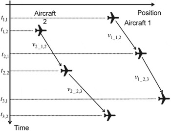
Figure 11. Calculation of the relative speed prediction error of two aircraft.

Since the relative speed prediction error (v ₁−v ₂) is calculated, the correlation between both errors is investigated. If two aircraft are sufficiently separated, their position and thus wind conditions differ significantly. In this research, the risk of collision for short separation (30 nm) is discussed, so the data of the pair which are closely separated are used. Here, the data where the distance between two aircraft is less than 100 nm is used.

In addition, according to assumption (a), both v ₁ and v ₂ vary with time, so it is expected that v ₁−v ₂ also depends on the position report interval. Like the calculation of f _v(v) only, the data when the position report interval is 27 minutes is used. To investigate the correlation, an orthogonal component of v ₁−v ₂, i.e. v ₁+v ₂, is also considered. If v ₁ and v ₂ are independent, v ₁−v ₂ and v ₁+v ₂ should have the same distribution. Figure 12 shows the relative frequency of v ₁−v ₂ and v ₁+v ₂. This figure clearly shows that v ₁−v ₂ has a narrower distribution than v ₁+v ₂. The SD of v ₁+v ₂ is also about 1·5 times larger than that of v ₁−v ₂. This means that v ₁ and v ₂ are dependent.

Figure 12. Relative frequency of v ₁−v ₂ and v ₁+v ₂ when the position report interval is 27 minutes.

With these two factors taken into consideration, it is expected that the risk of collision will be reduced and estimated more accurately.

4.2. Refined Calculation Method

To implement the two factors explained in the last chapter, the calculation method should be refined. First, assumption (b) is considered. To consider the relative speed prediction error, Equation (7) is replaced by the following expressions:

(15)$$\eqalign{P_x (x,\tau ) = & \int_0^T {\displaystyle{{dT_g} \over T}\int_0^{T + \tau} {\displaystyle{{dt} \over {T + \tau}} \int_{ - \infty} ^\infty {du\int_{ - \infty} ^\infty {dw}}}} \int_{ - x - \lambda _x} ^{ - x + \lambda _x} {d(\Delta X)} \cr & \times g_1* g_2 \left( {\Delta X\left( {t;\displaystyle{{u + w} \over {\sqrt 2}}, \displaystyle{{u - w} \over {\sqrt 2}}, T_g, T} \right)} \right)f_{v +} (u)f_{v -} (w)\left| {J(u,w)} \right|} $$

where J(u,w) is a Jacobian matrix, and $J(u,w) \equiv \displaystyle{{\partial (v_1, v_2 )} \over {\partial (u,w)}}$. $u = \displaystyle{{v_1 + v_2} \over {\sqrt 2}}, \;w = \displaystyle{{v_1  - v_2} \over {\sqrt 2}} $, and f _v+(u) and f _v−(w) indicate that the probability density function of u and w, respectively. The u-w coordinate system is an orthogonal rotational transformation of v ₁−v ₂ coordinate system, so |J(u,w)|=1.

However, there is one problem regarding the probability density function. If f _v+(u) and f _v−(w) are modelled by the Laplace distribution, f _v(v) should be possible to be calculated by the convolution of f _v+(u) and f _v−(w). However, the convolution of these two functions does not match the Laplace distribution. The convolution of two functions can be calculated by the following expressions:

(16)$$\eqalign{&\hskip-12pt\int {\,f_{v +} (u)f_{v -} (w)} du = \int {\,f_{v +} (u)f_{v -} (} \sqrt 2 v_1 - u)du = f_{v +} * f_{v -} (\sqrt 2 v_1 ) = f_v (\sqrt 2 v_1 ) \cr &\hskip-12pt f_v (v_1 ) = f_{v +} * f_{v -} (v_1 ) \cr = & \left( {\displaystyle{{\lambda _ +} \over {\lambda _ + - \lambda _ -}} + \displaystyle{{\lambda _ +} \over {\lambda _ + + \lambda _ -}}} \right)\displaystyle{{\exp \left( { - |v_1 - \mu _ + - \mu _ - |/\lambda _ +} \right)} \over {4\lambda _ +}} \cr &+ \left( {\displaystyle{{\lambda _ -} \over {\lambda _ - - \lambda _ +}}\cr + \displaystyle{{\lambda _ -} \over {\lambda _ - + \lambda _ +}}} \right)\displaystyle{{\exp \left( { - |v_1 - \mu _ + - \mu _ - |/\lambda _ -} \right)} \over {4\lambda _ -}}} $$

To investigate the shape of the convoluted function, the following substitutions are assumed: λ ₊=2λ and λ ₋=λ and μ ₋=μ ₊=0. The probability density function of f _v(v ₁) is shown in Figure 13. The Laplace distribution where $\lambda= \sqrt {\lambda ^2+ (2\lambda )^2} = \sqrt 5 \lambda $ is also shown so that the SD of the convoluted function and Laplace distribution is set the same. As seen from the figure, both functions have similar shapes. Both functions are almost log linear with v. The difference is found in the value around 0 and the tail. However, the reason why the Laplace distribution is chosen as the function describing the speed prediction error in the conventional method is that the Laplace distribution is a long-tailed distribution for conservative estimation, and there is no proof that the speed prediction error should follow the Laplace distribution. Therefore, if the speed prediction error has a similar form to the Laplace distribution, it is reasonable to model both u and w by the Laplace distribution.

Figure 13. Probability density function of Convoluted Function and Laplace Distribution.

Next, assumption (a) is considered. v ₁ and v ₂ are dependent on the position report interval, so it is expected that u and w are also dependent on time. Figure 14 shows the SD of u and w for each position report interval. The number of the obtained data sets is small except for the ten and 27 minutes position report interval, so they oscillate between the position report intervals. However, some trends are observed. The SD of u is almost constant throughout the position report interval. As for w, the SD tends to decrease gradually with the increase of the position report interval. Consequently, it is assumed that λ ₊ and λ ₋ are changed linearly with the position report interval. Therefore, the following equations are assumed:

(17)$$\eqalign{& \lambda _ + = \lambda _{0 +} + a_ + \Delta t \cr & \lambda _ - = \lambda _{0 -} + a_ - \Delta t} $$

where Δt indicates the position report interval with the unit of minutes. To fit the model, as for u, three parameters (λ ₀₊, a ₊, μ ₊) have to be set. Let u _i and t _i be the ith data of u and position report interval. The parameters are optimized to maximize the following expression via the maximum likelihood estimation.

(18)$$\sum {\log (\,f\,(u_i ;\mu _ \pm, \lambda _{0 \pm} + a_ \pm t_i ))} $$

The obtained parameters are summarised as follows:

(19)$$\eqalign{& \lambda _{0 +} = 5 {\cdot} 256,a_ + = 0 {\cdot} 0543,\mu _ + = - 2 {\cdot} 919 \cr & \lambda _{0 -} = 4 {\cdot} 960,a_ - = - 0 {\cdot} 0188,\mu _ - = - 0 {\cdot} 182} $$

According to the result, the deviation of u increases with time, and that of w decreases with time, as seen also in Figure 14. To confirm the result, Figure 15 shows the obtained fitted model on Figure 12. Both models fit the actual data well, and it is concluded that the parameters are well estimated. Besides, the increase of the speed prediction error (v ₁; shown in Figure 10) with time can also be explained such that the increase of u contributes the increase of v ₁, not contributed by w.

Figure 14. Relationship between standard deviation of u and w and position report interval.

Figure 15. Relative frequency and fitted models when the position report interval is 27 minutes.

However, the larger error of both u and w leads to a higher risk of collision, although the error of w affects the risk of collision more. Considering the fact that the collision is likely to happen when the time to the latest position report is more than the periodic position report interval, the decrease of SD of w with time means the risk of collision is estimated low. There is no proof that the distribution of w tends to decrease with time, so this time for the conservative risk estimation λ ₋ is assumed to be constant and its value is used at the position report interval being ten minutes (periodic position report interval), i.e. 4·960+10×(−0·0188)=4·772. In the same way, for the conservative risk estimation λ ₊ uses the data when the position report interval is 27 minutes, i.e. 5·256+27×0·0543=6·722.

4.3. Calculation of Risk of Collision Using the Refined Method

Using the values obtained in Section 4.2, the risk of collision is calculated based on Equation (15). The results are summarised in Table 4. Only the conditions mentioned in Section 4.2 are changed from the conventional method. The results show that in each periodic position interval, the risk of collision estimated by the refined method is obtained about ten times less than that by the conventional method. Even if 14 minutes position report interval is applied based on future traffic, the risk of collision is lower than the TLS. This result indicates that 14 minutes periodic position report interval can be introduced even if traffic volume increases and 30 nm separation standard is applied more often.

Table 4. Difference of risk of collision between calculation methods for each periodic position report interval based on future traffic.

4.4. Estimation of Data Exchange Cost Saving

Since the benefit of the extension of the periodic position report interval is the data exchange cost saving, here the expected saving is estimated. First, the number of the periodic position reports is obtained. This extension of interval is applied not only to the considered routes but also to all aircraft in the Fukuoka FIR, so all aircraft in this FIR are considered. According to the latest monthly information, ten minutes periodic position reports were sent 3,550 times on average per day, about 1·3 million times per year. If the position report is extended from ten minutes to 14 minutes, the number of position reports will decrease roughly by 4/14 times, so about 370,000 data exchanges will be reduced. If a single data exchange is assumed to cost one dollar, about 370,000 dollars can be saved per year. Under future traffic assumptions, the cost savings will be up to 910,000 dollars per year. Although this cost saving might seem small, this cost saving effect will last as long as the 30 nm separation standard exists, so there is no reason that the position report interval is kept low unnecessarily. Besides, if the position report interval is extended worldwide by using the proposed method, further data exchange costs will be reduced.