2. CHARACTERISATION OF THE ORBITAL AND CLOCK CORRECTIONS

While unbiased Global Navigation Satellite System (GNSS) observation errors in the open sky environment are typically modelled assuming that they have a normal distribution based on extensive testing (Misra and Enge, Reference Misra and Enge2006; El-Mowafy, Reference El-Mowafy2015a), currently a few studies discuss, with limited scope, characterisation of real-time GNSS orbit and clock corrections, for example, Hadas and Bosy (Reference Hadas and Bosy2015) and El-Mowafy et al. (Reference El-Mowafy, Deo and Kubo2017). In this section, a small contribution to this effort is made by briefly discussing two aspects; the statistical distribution of the IGS-RTS corrections, and estimating suitable values for their standard deviations. Understanding the distribution of these corrections is fundamental in forming the statistical criteria used in the detection and identification of their faults, and the standard deviations are needed in their stochastic modelling as quasi-observations. In this study, a 95% confidence interval is used in statistical testing.

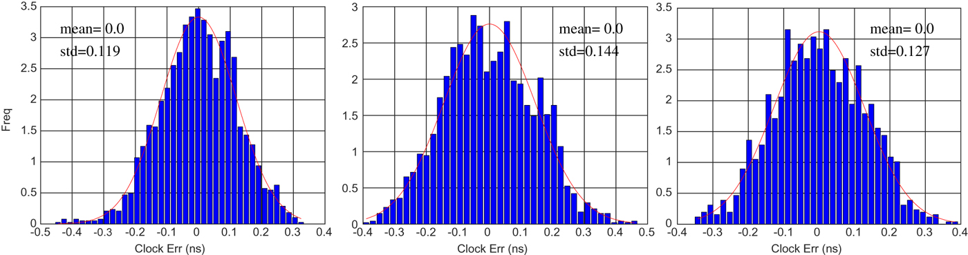
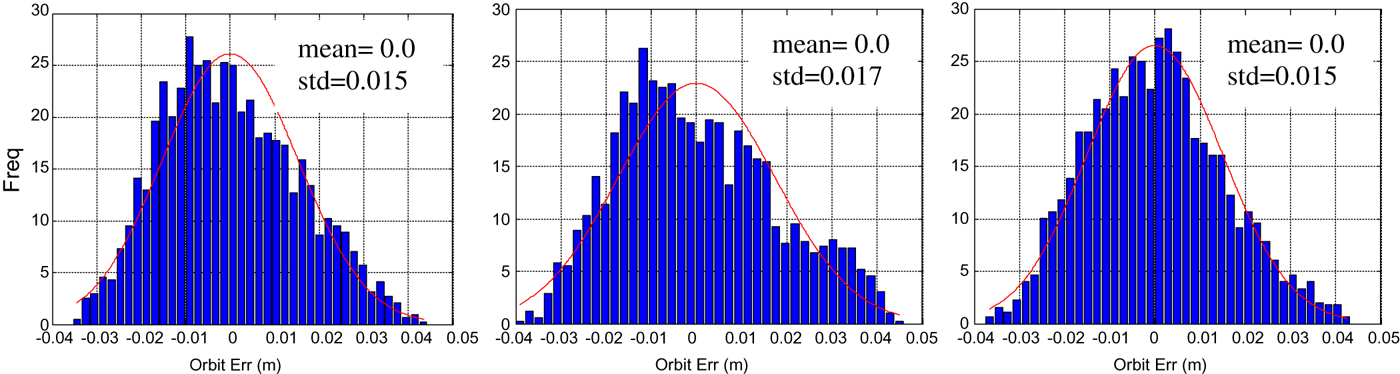
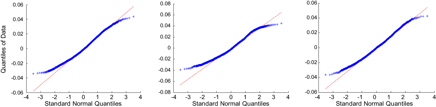
Six months of archived IGS-RTS orbital and clock corrections (January-June 2016) for all GPS satellites of the IGC01 stream available at 30 second intervals were analysed to estimate their stochastic properties. Firstly, the corrections were screened to detect possible outliers, where errors larger than a certain threshold were eliminated. Next, the data were de-trended to remove deterministic components such as biases and drifts, including the shift at each epoch between the used IGS-RTS reference analysis centre and the IGS timescales. Errors in the IGS-RTS orbit and clock corrections were next computed as the differences between the broadcast orbit and clock offset corrected by IGS-RTS products from the IGS final orbits and clock offset. The latter is taken as a reference since it has the most precise products currently available. The histograms of the errors were inspected and their Cumulative Distribution Function (CDF) were compared with possible best fits. In addition, their normality was checked using Q-Q plots, and results of Chi-square goodness of fit were analysed. For demonstration purposes, results of three representative satellites from the current three operational GPS blocks are shown: PRN16 (a typical satellite from Block IIR), PRN29 (Block IIRM), and PRN30 (block IIF). Their results are illustrated in Figures 1–6. Figure 1 shows the histograms of the clock corrections in addition to the normal distribution curve to see how close they are to each other. The mean of the errors and their standard deviations are given in nanoseconds (ns). Figure 2 depicts the Q-Q plot of the quantiles of the clock corrections with that of the standard normal. Figure 3 demonstrates the cumulative probability of the clock corrections, treated as a univariate, with their best fitted normal distribution, determined using the maximum likelihood method. Figures 4 to 6 show similar plots for the orbital corrections, where the mean of the errors and standard deviations are given in metres (m).

Figure 1. Histogram and normal distribution plot of IGS-RTS clock errors - PRN16-block IIR (left), PRN 29-block IIRM (middle), and PRN30-block IIF (right).

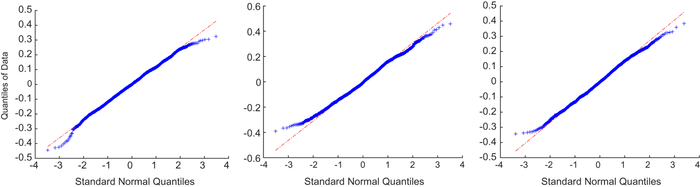
Figure 2. Q-Q plot of IGS-RTS clock errors - PRN16 (left), PRN 29 (middle), and PRN30 (right).

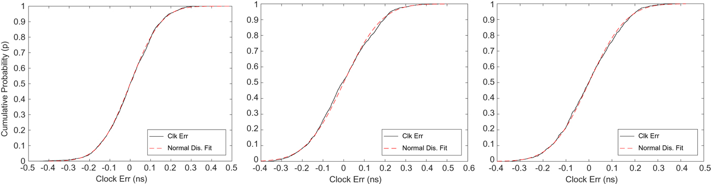
Figure 3. Cumulative probability fitting of data with normal distribution for IGS-RTS clock errors - PRN16 (left), PRN 29 (middle), and PRN30 (right).

Figure 4. Histogram and normal distribution plot of IGS-RTS orbit errors - PRN16-block IIR (left), PRN 29-block IIRM (middle), and PRN30-block IIF (right).

Figure 5. Q-Q plot of IGS-RTS orbit errors - PRN16 (left), PRN 29 (middle), and PRN30 (right).

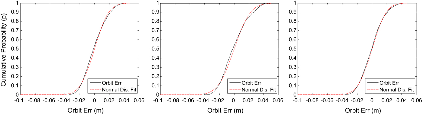
Figure 6. Cumulative probability fitting of data with normal distribution for IGS-RTS orbit errors - PRN16 (left), PRN 29 (middle), and PRN30 (right).

With a focus on fitting the data at the central area of the distribution, the clock error plots show that their distribution can approximately follow the normal distribution. The histograms were very close to the normal curves; the Q-Q plots showed a good fit for the 95% confidence interval and their cumulative probability matched well with the normal distribution. The Chi-square goodness of fit test passed for all clock corrections of all satellites, with P-values ranging between 0.3-0.4, which is larger than the selected 0.05 threshold. The orbit Q-Q plots show good agreement up to ±2 quantiles (95% confidence interval) but with some divergence for the tails above that value, with good agreement of the CDF fit and the histograms with the normal distribution. The Chi-square goodness of fit test did not pass for all satellites, and thus requires further analysis. Overall, from a practical point of view and as per the central limit theorem, it is reasonable to assume a normal distribution for the stochastic properties of the clock and orbit corrections using a 95% confidence interval.

The accuracy of the orbit and clock corrections were next analysed in terms of the mean of their absolute error values and the Root-Mean-Square Error (RMSE) for all GPS satellites over a long period (six months). These values are given in Table 1, which shows that the negative and positive errors are balanced (that is, no bias), and the average of the absolute values of errors for the orbit and clock corrections were 0.041 m and 0.281 ns, respectively. These results agree with the published values of the IGS-RTS monitoring utility. Such stochastic information will be needed when weighting the corrections as quasi-observations and in the FDE process if this information is not provided (by IGS-RTS for example).

Table 1. Accuracy of IGS-RTS products during the study period (January-June 2016). Error is computed as the difference between IGS-RTS corrected orbits and clocks and IGS-final products.

3. A MODIFIED PPP MODEL USING THE ORBIT AND CLOCK CORRECTIONS AS QUASI-OBSERVATIONS

In this section, modelling of the orbit and clock corrections as additional ‘quasi’ observations in the PPP model is discussed. The un-differenced observation equations for pseudorange code and carrier-phase measurements using the broadcast navigation message for satellite s from a GNSS constellation, such as GPS, to receiver r for signal frequency i in length units (m) can be formulated as:

(1)$$P(i)_{r}^{s}=\rho_{r}^{s}+\cos \lpar \theta\rpar d\rho^{s}+c\lpar dt_{r}-dt^{s}+d_{r}\lpar i \rpar -d^{s}\lpar i \rpar \rpar +m_{r}^{s}\,T+\mu_{i}\,I^{s}+\varepsilon_{{P(i)}_{r}^{s}}$$

(2)$$\eqalign{\phi (i)_{r}^{s}&=\rho_{r}^{s}+\cos \lpar \theta \rpar d\rho^{s}+c\lpar dt_{r}-dt^{s} \rpar +\delta_{r}\lpar i \rpar -\delta^{s}\lpar i \rpar +m_{r}^{s} T-\mu_{i} I^{s}\cr & \quad +\lambda_{i} N_{r}^{s}\lpar i \rpar +\varepsilon_{{\phi (i)}_{r}^{s}}}$$

where $P(i)_{r}^{s}$ and $\phi (i)_{r}^{s}$ denote code and carrier-phase measurements, respectively, c is the speed of light in a vacuum and $\rho_{r}^{s}$ is the satellite-to-receiver geometric range. dρ^s is the Three-Dimensional (3D) satellite orbital error, defined as the difference between the actual satellite position and its position computed from the broadcast message. It is projected along the receiver-to-satellite slant line using $\cos \lpar \theta \rpar $, where θ is the angle between the orbital error vector and the line of sight. dt _r and dt ^s are the receiver and satellite clock offsets respectively and T is the zenith troposphere delay modelled as one vertical component for all satellites projected along the receiver-to-satellite line of sight using a mapping function $\rm{m}_{r}^{s}$ (Tuka and El-Mowafy, Reference Tuka and El-Mowafy2013). Alternatively, the hydrostatic component can be modelled out using an empirical model and only the wet component is estimated. The model can be augmented to include troposphere gradients along the East-West and North-South directions. λ_i denotes the wavelength, I is the slant ionosphere delay for a reference frequency, for example, L1 for GPS, $\mu_{i}={f_{1}^{2}\over f_{i}^{2}}$ is the dispersive coefficient of the ionosphere with respect to the reference frequency and $N_{r}^{s}\lpar i \rpar $ is the integer ambiguity. $d_{r}\lpar i \rpar $ and $d^{k}\lpar i \rpar $ are the receiver and satellite code observation hardware delay (bias) in time units and $\delta_{r}\lpar i \rpar $ and $\delta^{k}\lpar i \rpar $ are the receiver and satellite phase observations hardware delay (bias) including the initial phase biases expressed in metres. $\varepsilon_{{P(i)}_{r}^{s}}$ and $\varepsilon _{{\phi (i)}_{r}^{s}}$ comprise measurement noise and multipath of code and phase measurements.

To eliminate the first-order ionosphere delay, usually the ionosphere-free combination (IF) is used, and the un-differenced ionosphere-free code and observations can be expressed as:

(3)$$P(IF)_{r}^{\rm{s}}=\rho_{r}^{\rm{s}}+EC_{r}^{s}+c \overline{dt}\lpar IF \rpar _{r}+m_{r}^{s}\,T+\varepsilon_{{P(IF)}_{r}^{\rm{s}}}$$

(4)$$\phi (IF)_{r}^{\rm{s}}=\rho_{r}^{\rm{s}}+EC_{r}^{s}+ c \overline{dt}(IF)_{r}+m_{r}^{s}T+\lambda_{IF} \tilde{N}_{r}^{\rm{s}}(IF)+\varepsilon_{{\phi (IF)}_{r}^{\rm{s}}}$$

where:

(5)$$EC_{r}^{s}=\cos \lpar \theta \rpar d\rho^{s}-c \overline{dt}\lpar IF \rpar ^{s}$$

The terms $c\overline{dt}\lpar IF \rpar ^{s}$, $c\overline{dt}(IF)_{r}$ and $\lambda_{\rm{IF}}\tilde{N}_{r}^{\rm{s}}(IF)$ include the biases as explained in the Appendix, and $EC_{r}^{s}$ combines both the orbit and satellite clock corrections along the line of sight for each satellite.

In the proposed approach, the observation vector of the code and phase observations and their covariance matrices (denoted as Q _P and Q _ϕ) are augmented to include an additional ‘quasi’ observation $\widetilde{EC}_{r}^{s}=\rm{cos}(\theta)d\tilde{\rho}^{s}-c\widetilde{dt}^{s}$ for each satellite, where $d\tilde{\rho}^{s}$ and $\widetilde{dt}^{s}$ denote the acquired IGS-RTS orbit and clock corrections. Its observation equation is expressed as:

(6)$$\widetilde{EC}_{r}^{s}=EC_{r}^{s}+\varepsilon_{\widetilde{EC}_{r}^{s}}$$

$\varepsilon_{\widetilde{EC}_{r}^{s}}$ is the noise in $\widetilde{EC}_{r}^{s}$ and $\cos \lpar \theta \rpar $ is the projector of the 3D orbital error on the range space. It is computed from the satellite precise position (x ^s), its broadcast position ($x^{\rm{bdcst}}$) is estimated from the broadcast navigation message, and the user approximate position (X_u) where:

(7)$$\cos (\theta )={\overrightarrow{\lpar x^{s}-x^{\rm{bdcst}}\rpar }\cdot \overrightarrow{(x^{s}-X_{u})}\over{\left\| x^{s}-x^{\rm{bdcst}} \right\|\left\| x^{s}-X_{u} \right\|}}$$

x ^s is computed in RT as follows. The IGS-RTS orbit corrections in the Radio Technical Commission for Maritime Services (RTCM) - State Space Representation (SSR) format are provided in terms of the radial, along-track and cross-track components, denoted as $\delta \rho_{r}$, $\delta \rho_{a}$ and $\delta \rho_{c}$ respectively, in addition to their velocities ($\delta \dot{\rho}_{r}$, $\delta \dot{\rho}_{a}$ and $\delta \dot{\rho}_{c}$). The orbit corrections at time t are computed using the broadcast navigation message with a reference time t _o as follows (Hadas and Bosy, Reference Hadas and Bosy2015; El-Mowafy et al., Reference El-Mowafy, Deo and Kubo2017):

(8)$$\delta \tilde{\rho}=[\delta \rho_{r}\; \delta \rho_{a}\; \delta \rho_{c}]^{T}+ [\delta \dot{\rho }_{r}\; \delta \dot{\rho}_{a}\; \delta \dot{\rho}_{c}]^{T} (t-t_{o})$$

These corrections are transformed to geocentric corrections by applying the radial, along-track and cross-track unit vectors (e _r, e _a and e _c) and are next added to the broadcast orbit x ^brdcst to give the final precise orbit x ^s:

(9)$$x^{s}= x^{brdcst}+ {diag}(e_{r}\; e_{a}\; e_{c})\delta \tilde{\rho}$$

The satellite clock correction (including the ionosphere-free code biases) is given as a range correction in terms of a quadratic polynomial with coefficients (q0, q1, q2) such that:

(10)$$c\overline{\delta t} = q0 + q1 \lpar t-t_{o} \rpar +q2\lpar t-t_{o} \rpar ^{2}$$

and the corrected satellite clock offset is expressed as:

(11)$$c\widetilde{dt}^{s}=c\, t^{brdcst}+ c\overline{\delta t}$$

where t ^brdcst is the GNSS satellite clock offset computed from the broadcast message, and finally the term $\widetilde{EC}_{r}^{s}=\rm{cos}(\theta )d\tilde{\rho}^{s}-c\widetilde{dt}^{s}$ is computed using Equations (7), (8) and (11).

Using GPS as an example, the linearized fault-free measurement model using all satellites in view is given as:

(12)$$y = H x +\varepsilon$$

where y and x are the vectors of observations and unknowns, respectively, H is the design matrix and ε denotes the noise. Combining the observation Equations (3), (4) and (6), the final system of observation equations for n GPS satellites after re-arrangement of the states is expressed as:

(13)$${\underbrace{\left(\matrix{P(IF)_{r}^{\rm{s}} \cr \phi(IF)_{r}^{\rm{s}}\cr \widetilde{EC}_{r}^{s}}\right)}\limits_y}={\underbrace{\left(\matrix{G & u & m &0 & u \cr G & u & m & \lambda_{IF}\times \hbox{I} & u \cr 0 & 0 & 0 &0 & u}\right)}\limits_{H}} {\underbrace{\left(\matrix{X_{u}\cr c\overline{dt}(IF)_{r}\cr T\cr \tilde{N}_{r}^{s}(IF)\cr {EC}_{r}^{s}}\right)}\limits_{x}} \quad + \varepsilon\qquad \hbox{for}\ s = 1\ \hbox{to}\ n$$

where only the corrections of the used satellites are considered. The design matrix H is full rank, where G is the geometry (direction-cosine) matrix computed from broadcast ephemeris with dimension n×3, I is the identity matrix of dimension n, u is a unit vector of ones and m is a column vector representing the line-of-sight troposphere mapping function. The vectors u and m have dimension n×1. The number of unknowns equals (5+2 n), where 5 refers to the common unknowns (X _u, $c\overline{dt}_{r}$, T) and each satellite has $\lpar EC_{r}^{s},\tilde{N}_{r}^{s} \rpar $ states, and with a total number of observations equalling 3n, this system can be solved using observations from five satellites similar to the case of conventional PPP.

Possible unknown RT biases in $\widetilde{EC}_{r}^{s}$, which can be denoted as $d\widetilde{EC}_{r}^{s}$, such as the time shift between the analysis centre and IGS time scales and the average of the shift between the orbit corrections from the correct values (which can be defined, e.g. with respect to the reference IGS final orbits) are added to the common receiver clock offset that is estimated in each epoch. Hence, $c \overline{dt}(IF)_{\rm{r}}= c(dt\lpar IF\rpar _{\rm{r}}+{DCB}_{\rm{r}}\lpar IF\rpar ) + d\widetilde{EC}_{r}^{s}$ (see Appendix).

For the stochastic model, the proposed approach is advantageous in the sense that it includes the full uncertainty information of the precise orbit and clock corrections when being estimated. The variance of the term $\widetilde{EC}_{r}^{s}$ is computed as:

(14)$$\sigma_{\widetilde{EC}_{r}^{s}}^{2}={\rm{cos}}^{2}(\theta)\, \sigma_{d\tilde{\rho}^{s}}^{2}+ \sigma_{c\widetilde{dt}^{s}}^{2}-2 \sigma_{\cos (\theta)d\tilde{\rho}^{s}, c \widetilde{dt}^{s}}$$

where $\sigma_{d\tilde{\rho}^{s},c\widetilde{dt}^{s}}$ is the covariance, $\sigma_{d\tilde{\rho}^{s}}$ and $\sigma_{c\widetilde{dt}^{s}}$ are the Standard Deviations (STDs) of the orbit and clock corrections, which can be provided in the RTCM-SSR message, or alternatively determined from the STDs of their components using Equations (7), (8) and (10) by applying the covariance propagation law. This information can be provided by the analysis centre as a priori values, for instance as the average values over a certain period, for example, 1-2 hrs, that is close to the observation time. Alternatively, if the STDs are not provided, they can be assumed based on data characterisation presented in the previous section with conservative values such as $\sigma_{d\tilde{\rho}}= 5$ cm and $c\widetilde{dt}\lpar IF\rpar ^{s}=0.22$ ns, and using an empirical correlation factor (R), which can be estimated from analysis of the corrections, such that $\sigma_{d\tilde{\rho}^{s},c \widetilde{dt}^{s}}=5\,\rm{cm} \times 0.22\,\rm{ns}\times R$. The observation covariance matrix is expressed as $Q_{y}={diag}(Q_{P_{r}^{\rm{s}}}, Q_{\phi_{r}^{\rm{s}}}, Q_{\widetilde{EC}^{s}})$, for s=1 to n. The sub-covariance matrices $Q_{P_{r}^{\rm{s}}}$ and $Q_{\phi_{r}^{\rm{s}}}$ are typically assumed diagonal for the observed satellites, with a priori values as shown in El-Mowafy (Reference El-Mowafy2015b) weighted using an arbitrary satellite elevation-angle dependent model, and uncorrelated code and phase observations. $Q_{\widetilde{EC}^{s}}$ is uncorrelated with $Q_{P_{r}^{\rm{s}}}$ and $Q_{\phi_{r}^{\rm{s}}}$ due to the fact that the IGS corrections are independent from the user observations since they are being estimated from a different set of observations collected at the IGS reference stations. Finally, if no correlation information is given between the $\widetilde{EC}_{r}^{s}$ (and their components) among different satellites, their covariance can be either assumed or ignored such that $Q_{\widetilde{EC}^{s}}$ becomes diagonal.

4. DETECTION AND IDENTIFICATION OF FAULTY OBSERVATIONS

In a pre-processing step, the observations should be screened to detect severe irregularities and exclude faulty observations, and if necessary repair them (e.g. in the case of cycle slips). At the analysis centre, the precise orbit and clock corrections are estimated in one process, and hence a fault in one will typically result in a fault in the second. Accordingly, in the proposed method, the combined orbit and clock corrections term for each satellite is treated as one quasi-observation, which undergoes the screening process and is examined with a combined probability of fault occurrence. As mentioned above, faults during analysis centre processing are rare, but the user has to be able to detect faults for critical real-time applications, in particular faults induced by spoofing and meaconing.

In the presence of large errors (or faults), the error state vector, denoted as ∇, is included in the observation model, which is expressed as:

(15)$$y=H\, x+ C\nabla +\varepsilon$$

where for m number of observations (including $P_{r}^{\rm{s}}$, $\phi_{r}^{\rm{s}}$ and $\widetilde{EC}_{r}^{s}$ for all satellites), C is a fault locality matrix that has a dimension $m\times \gamma$, where γ is the number of errors in ∇. This number should be less than the degrees of freedom (df) in order to enable detection of faults, such that $1\le \gamma \le df$, where df corresponds to the number of satellites above five as explained earlier. Each column of C has a one in the index corresponding to the observation assumed to be affected and zeros elsewhere. Due to the correlation among code and phase errors, cycle slips of phase observations are first detected and repaired and next code outliers are detected and removed (El-Mowafy, Reference El-Mowafy2014). Cycle slip detection can be performed using geometry-free single-satellite time difference of the between-phase observations from two frequencies or the time-rate of the ionosphere delay. In this paper, the data of each epoch are screened (known as local testing) using least squares. Next, the clean data set is processed in PPP using an extended Kalman filter as described in the next section.

The size of the error that can be detected with a certain probability of false alarm (α) and miss-detection (β) is known as the Minimal Detectable Bias (MDB), such that for observation j, it is expressed as (De Bakker et al., Reference De Bakker, Van der Marel and Teunissen2009):

(16)$$MDB_{j}=\sqrt{\lambda_{o}\over{C^{T}Q_{y}^{-1}Q_{\hat{e}}Q_{y}^{-1}C}}$$

where λ_o is the non-centrally parameter (see Aydin and Demirel, Reference Aydin and Demirel2005), which is a function of α and β. Utilising the observation residuals, the best estimator of the error vector ($\hat{\nabla}$) can be determined from (El-Mowafy, Reference El-Mowafy2014):

(17)$$\hat{\nabla}=(C^{T}Q_{y}^{-1}Q_{\hat{e}}Q_{y}^{-1}C)^{-1}C^{T}Q_{y}^{-1}\hat{e}$$

with its covariance matrix as:

(18)$$Q_{\hat{\nabla}}=(C^{T}Q_{y}^{-1}Q_{\hat{e}}Q_{y}^{-1}C)^{-1}$$

where ê and Q _ê are the computed observation residuals and their covariance matrix is computed as $Q_{\hat{e}}=Q_{\rm{y}}-[H(H^{T}Q_{\rm{y}}^{-1}H)^{-1}H^{T}]$. The matrix C is set to test all possibilities of the presence of errors in the observations. In the case of a single fault in the observations, that is q=1, C reduces to a column vector c, and $\hat{\nabla}$ turns into a scalar.

A quick method for detection of errors is to apply the Uniformly Most Powerful Invariant (UMPI) test. Under the assumption that ê has a zero-mean with Gaussian distribution in the fault-free unbiased mode, the statistic ($\hat{\nabla }^{T}Q_{\hat{\nabla }}^{-1}\hat{\nabla}$) will have a Chi-square distribution; therefore, observation errors are suspected, when (Teunissen, Reference Teunissen2006):

(19)$$\hat{\nabla}^{T}Q_{\hat{\nabla}}^{-1}\hat{\nabla}\ge \chi_{\alpha 1}^{2}(df,0)$$

where $\chi_{\alpha 1}^{2}\lpar df,0\rpar $ is the threshold Chi-square value for α 1 and df. If the test fails, one needs to identify and exclude the suspected observations corresponding to these faults.

Under the assumption that the un-biased observation errors in the fault-free mode are Gaussian with zero-mean, the normalised form for $\hat{\nabla}_{j}$ for observation j is:

(20)$$w_{j}={\hat{\nabla}_{j}\over{\sigma_{\hat{\nabla}_{j}}}}$$

which should follow a standard normal distribution where $\sigma _{\hat{\nabla }_{j}}$ is the standard deviation of $\hat{\nabla }_{j}$ (Baarda, Reference Baarda1968). w is ranked for all observations and the observation j is suspected to contain a fault when:

(21)$$\vert w_{j}\vert \ge N_{\alpha\over 2}(0,1) \quad |w_{j}|\ge |w_{k}|\quad \hbox{for}\ k= 1\ \hbox{to}\ m$$

and may be excluded. Note that the significance level α for the w-statistic is different from the significance level α 1 for the UMPI detection test. The latter can be computed using Baarda's B method (Baarda, Reference Baarda1968), which assumes the same probability for a type II error (failure to reject a false null hypothesis) in both the detection and identification tests. In this paper, the total significance level is selected as 0.05, and is assumed equally distributed among the observations; hence, α=0.05/number of observations. The UMPI test is re-applied after exclusion of faulty observations to check whether it would be successful after removing the suspected observation(s).

The correlations among observation errors should also be considered as this may cause one error to mask other errors. For observations k and j, the correlation coefficient between their corresponding errors denoted as $\xi_{{\hat{\nabla}}_{k},\hat{\nabla}_{j}}$ reads:

(22)$$\xi_{\hat{\nabla }_{k},\hat{\nabla }_{j}}={c_{k}^{T}Q_{y}^{-1}Q_{\hat{e}}Q_{y}^{-1}c_{j}\over{\sqrt {c_{k}^{T}Q_{y}^{-1}Q_{\hat{e}}Q_{y}^{-1}c_{k}} \sqrt{c_{j}^{T}Q_{y}^{-1}Q_{\hat{e}}Q_{y}^{-1}c_{j}}}}$$

where c _k and c _j are zero column vectors except for the elements corresponding to the observations k and j which equal 1. Hence, if a high correlation coefficient is present for a suspected observation with other observation errors, one will need to carefully inspect and consider exclusion of its correlated observations. Fortunately, code outliers are typically uncorrelated (El-Mowafy, Reference El-Mowafy2014; Reference El-Mowafy2015a); therefore, if cycle slip detection and repair is performed successfully, the probability of one faulty observation masking another observation that could also be faulty is low. However, for the combined orbit and clock correction terms among different satellites, the correlation coefficient has to be closely monitored.

In the case of using a limited number of observations, unnecessary exclusion of observations may affect positioning performance; therefore, an additional confirmation check is applied based on the solution separation method (Blanch et al., Reference Blanch, Walter, Enge, Wallner, Fernandez, Dellago, Ioannides, Hernandez, Belabbas, Spletter and Rippl2013; Joerger et al., Reference Joerger, Chan and Pervan2014; El-Mowafy, Reference El-Mowafy2017). In this check, the solution of the unknown position using all observations is:

(23)$$\hat{x}= S\, y$$

where $S=(H^{T}\, Q_{y}^{-1}\, H)^{-1}\, H^{T}\, Q_{y}^{-1}$ using least squares. For a potential fault in observation j (which could be more than one observation as per the tested fault mode), S is recomputed as S _j by excluding this observation where:

(24)$$S_{j}=(H^{T}(A_{j} Q_{y}^{-1}) H)^{-1}\, H^{T} (A_{j}Q_{y}^{-1})$$

and the corresponding solution is $\hat{x}_{j}=S_{j}y$, where A _j is a reformed identity matrix of dimension m such that the diagonal element corresponding to the suspected faulty observation is zero. The test statistic is the difference between the all-observations solution vector and the solution vector obtained by excluding observation j, that is $\vert \hat{x}-\hat{x}_{j}\vert$.

The STDs of the components of position differences in $\vert \hat{x}-\hat{x}_{j}\vert $, i.e. $\sigma_{{dE}_{j}}$, $\sigma _{{dN}_{j}}$, $\sigma_{{dU}_{j}}$ in the East, North and Up coordinates (E, N, U) in a local-level frame, can be expressed as:

(25)$$\sigma_{q,j}=\sqrt{a_{q}^{T}\,\lpar S_{j}-S \rpar \,Q_{y}(S_{j}-S)^{T}a_{q}}$$

where $q=\it{1,\, 2,\, 3}$ corresponds to dE _j, dN _j, dU _j respectively, such that $\sigma_{1,j}=\sigma_{{dE}_{j}}$ for which $a_{1}^{T}=\lsqb 1,\, 0,\, 0 \rsqb $, similarly $\sigma_{2,\,j}=\sigma _{{dN}_{j}}$ with $a_{2}^{T}=\lsqb 0,\, 1,\, 0 \rsqb $ and $\sigma _{3,j}=\sigma_{{dU}_{j}}$ with $a_{3}^{T}=\lsqb 0,\, 0,\, 1 \rsqb $. The null hypothesis of the test is H _o: ${\vert \hat{x}- \hat{x}_{j}\vert_{q}\over{\sigma_{q,j}}}\sim N_{\alpha 2\over{2}}(0,1)$. One can reject H _o in favour of the alternative hypnosis and assume confirmation of a faulty observation(s) j, if for any q:

(26)$${\vert \hat{x}-\hat{x}_{j}\vert_{q}\over \sigma_{q,j}}\ge N_{{\alpha 2}\over{2}}(0,1)$$

where $N_{\alpha 2\over 2}(0,1)$ is the inverse of the complement of the one-sided standard normal cumulative distribution function. Assume the same total probability of false alarm (0.05), which is presumed equally distributed for the horizontal and vertical components; $\alpha 2 = 0.05/\break (2 \times$ number of fault modes considered). The fault modes include the possibility of faults in any observation as well as in any possible significant combination of observation faults. Figure 7 shows a simplified flowchart of the basic steps considered in the testing and data fusion of the proposed method.

Figure 7. Flowchart of the basic steps in the testing and data fusion of the proposed method.

5. EVALUATION OF THE PROPOSED METHOD

In this section, a practical application of the proposed method is demonstrated. The method was applied at two IGS stations; PERT (Australia) and PTBB (Germany). The data spanned three days, 2 to 4 January 2017, with a 30 seconds sampling interval. The observations comprised ionosphere-free combinations of dual-frequency GPS data processed in a float-ambiguity PPP mode post-mission, assuming RT processing and using a Kalman filter with design parameters as shown in Table 2. The IGS-RTS IGC01 stream was used, which is a single-epoch combination solution for GPS orbit and clock corrections. The method is applicable to all RTS streams (IGC01, IGS01, IGS02, and IGS03), where the first is selected as a representative example. To evaluate the proposed method, its positioning accuracy was compared to the accuracy obtained using a traditional PPP method, processing the same data and corrections in the two methods.

Table 2. Kalman Filter design of the used PPP model.

Figure 8 shows a time series of the position errors in the East (E), North (N) and Up (U) coordinates in the local-level frame using the proposed method. The PPP errors are defined as the difference between the known station coordinates and PPP-determined positions. Table 3 shows the positioning accuracy in terms of the average of the absolute values of the errors after the solution converged. Results show that when using the proposed model, the error was within ±0.2 m, and mostly within ±0.1 m. The precision was at the sub-decimetre level. As the top row of Table 3 shows, the improvement due to including the full covariance information of the corrections was marginal, at the order of approximately 4–6% compared to the traditional PPP solution during the periods that are free from faults. However, this does not improve the convergence time of the PPP solution, which ranged between 30 to 40 minutes, as this time is dependent on factors such as precision of code measurements, satellite geometry and its change with time, number of frequencies used and number of observations.

Figure 8. Positioning Accuracy – stations PERT (left) and PTBB (right) during 2 January 2017 (top), 3 January 2017 (middle), and 4 January 2017 (bottom).

Table 3. Average positioning errors over three days of testing using the proposed method and traditional PPP (m). In the traditional method, faulted combined observations and corrections were excluded, whereas in the proposed approach the observations were kept and predicted corrections were used in place of the excluded corrections.

However, the advantage of the proposed method is clear when there are faults. Recall that conventional PPP methods combine the measurements with the orbit and clock corrections in one term and the FDE process is traditionally performed using a modified form of Equations (19)–(21) to check the observation residuals. If faults are detected in the corrected observations, both the observations and the corresponding corrections are excluded. Hence, faults in the corrections will result in exclusion of the observations. This will degrade positioning accuracy if a significant number of observations are eliminated, such as during spoofing or a meaconing attack. However, in the proposed method, faults in the corrections can be identified in a separate way from the observation faults. Hence, the observations are still usable if they are error-free and only faulty corrections are excluded, which would be replaced by predicted values as described in El-Mowafy et al. (Reference El-Mowafy, Deo and Kubo2017). This can be performed by the user or by a service provider. In this prediction approach, either the Holt-Winters method is applied for prediction of orbital corrections or the IGS ultra-rapid predicted orbits are used, and a linear or quadratic polynomial with sinusoidal functions is implemented for prediction of clock corrections. The prediction is independently performed for each satellite, and thus the orbit and clock corrections for all satellites in view can be predicted. Using this method, the predicted corrections would be accurate to a few cm for several minutes up to one hour of prediction. Accordingly, positioning can be maintained at decimetre-level accuracy (for full details, see El-Mowafy et al., Reference El-Mowafy, Deo and Kubo2017). To reduce the computational load, the process can be performed at a suitable time interval depending on the application, for example, every 10 minutes. If the number of outliers is more than the degrees of freedom, positioning will not be available using traditional PPP. However, with the proposed method, this case can be taken into consideration and checking can include a fault mode where all corrections are considered to be faulty. Once detected, these corrections are replaced by their predicted values for all satellites, which would allow continuity of positioning. A positioning accuracy of <20 cm can be maintained for 1 hr of prediction (El-Mowafy et al., Reference El-Mowafy, Deo and Kubo2017).

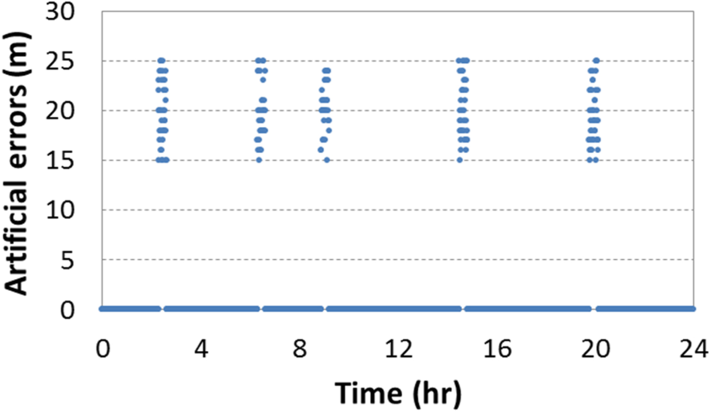
To demonstrate the power of the proposed method, a meaconing attack is assumed in the above test data, and random artificial errors ranging between 15 m and 25 m were inserted in the corrections for five periods. Each lasts for 20 minutes (totalling 200 incidents of faults/day) for the data used at each of the two test sites. As an example, Figure 9 shows the artificial errors inserted in one satellite's data from PERT on 2 January 2017, where each of the shown five periods lasts for 20 minutes. Note here that the size of the error does not really matter as long as it is above the test threshold, and 15–25 m can be assumed. The tests were repeated, using the same data, four times, each time representing a specific test scenario. In the first scenario, the artificial errors were inserted in only one satellite, and in the second scenario in two satellites. In the third test scenario, errors were inserted in three satellites, and in the final scenario they were inserted in all satellites. The latter fault mode represents a case of a full meaconing attack. The number of observed GPS satellites during these periods ranged between seven and nine satellites. The FDE performance and positioning results of the proposed method and a conventional PPP were compared and they were processed independently for each of these fault modes. The overall average of their absolute positioning errors for the two test sites over the three days of testing are given in Table 3, in rows 2-5.

Figure 9. Example of artificial errors inserted in one satellite for station PERT on 2 January 2017.

Both the proposed method and the traditional PPP were able to detect the presence of faults. The main difference is that the associated observations were excluded in the conventional PPP, and hence its positioning accuracy degraded sharply as the number of outliers increases due to the fact that more observations were eliminated (noting that the number of observations was limited since only GPS was used). For the case of a complete meaconing attack where all corrections were faulty, positioning was totally disabled in traditional PPP. On the other hand, with the proposed method all observations were used together with the predicted corrections during the periods of detected faults in the corrections, including the scenario for which all corrections were faulty. Accordingly, positioning was maintained all the time, as depicted in Table 3, with a small degradation of accuracy with the increase in the number of faulty corrections due to the use of more predicted corrections.

6. CONCLUDING SUMMARY

A new PPP model is proposed where combined orbit and clock corrections are treated as additional quasi-observations. This approach has two advantages. The first is that it includes both the variance and covariance information of the precise orbits and clock corrections, and can thus slightly improve positioning performance compared with traditional PPP methods that may only include the variance of the corrections. The second, which is a noteworthy benefit compared to conventional PPP methods, is that the proposed method allows FDE of the precise orbits and clock corrections in a separate way from the observations. The traditional methods combine the measurements with the orbit and clock corrections in one form, and screen the residuals of the corrected observations to detect faults. If faults are detected in the combined term, both the observations and the corresponding corrections are excluded. Hence, faults in the corrections will result in the exclusion of observations. This will significantly degrade positioning accuracy. However, in the proposed method, faults in the corrections can be identified separately from those of the observations. Thus, the observations are still usable and only the corrections can be excluded and replaced by predicted values that have an accuracy of a few cm when predicting for a short to medium period of time, for example, one hour. Therefore, PPP positioning accuracy is maintained with a slight decay.

Another contribution of this article is the characterisation of six months of IGS-RTS data, which showed that in practice one may assume a normal distribution for the clock and orbit corrections using a 95% confidence interval. Hence, consistent models can be applied when using the orbit and clock corrections as quasi-observations along with GNSS measurements, where errors of these measurements are typically assumed to have a normal distribution.

The practical application of the proposed method was evaluated at two IGS sites using dual-frequency GPS observations and IGS-RTS corrections. The data was processed in a float-ambiguity PPP scheme. For the tested data sets, positioning accuracy using the proposed method shows a marginal improvement of 4-6% over a traditional PPP algorithm. However, the main advantage is apparent when a meaconing attack is assumed with artificial errors inserted in one satellite, two satellites, three satellites and all satellites in view in independent tests for 20 minute periods at five variable times for each of the two test sites. While both the proposed method and traditional PPP were able to detect the faults, the conventional PPP positioning accuracy degraded sharply as the number of outliers increased since more observations were excluded until positioning was totally disabled when all corrections where faulty. On the other hand, with the proposed method, positioning was maintained with reasonable accuracy during these periods as all observations were used along with predicted values of the corrections that replaced the faulty ones.