2. GPS/GLONASS/GALILEO/BEIDOU VELOCITY ESTIMATION PROCEDURES

We begin with a brief review of the NVA algorithms as presented in Salazar et al. (Reference Salazar, Manuel, Jose, Jaume and Angela2011). We explain, to our understanding, the general ideas developed in this reference. For details, the interested reader is referred to the original paper. We then explain what has to be changed if not only GPS data are processed, as in Salazar et al. (Reference Salazar, Manuel, Jose, Jaume and Angela2011), but also GLONASS, Galileo and BeiDou.

Let:

(1)$${\bf x} = \left( {\matrix{ {\xi_1} \cr {\xi_2} \cr {\xi_3} \cr } } \right)\;\hbox{and}\;{\bf y} = \left( {\matrix{ {\eta_1} \cr {\eta_2} \cr {\eta_3} \cr } } \right)$$

be two three-dimensional column vectors (positions). With:

(2)$${\bf x}\cdot {\bf y} = \xi _1\eta _1 + \xi _2\eta _2 + \xi _3\eta _3,\quad \rho = \vert {\bf x} \vert = \sqrt {{\bf x}\cdot {\bf x}} \quad \hbox{and}\quad {\bf e} = \displaystyle{{\bf x} \over { \vert {\bf x} \vert }}$$

where x · y means the scalar product of the two vectors x and y, ρ denotes the Euclidian length of x and e is the unit vector in direction x. We assume that the vector x depends on the time t and has continuous derivatives up to the second order. The derivatives $\dot{\rho}$ and $\ddot{\rho}$ are obtained via elementary calculus:

(3)$$\dot p = \displaystyle{d \over {dt}} \vert {\bf x} \vert = \displaystyle{{{\bf x}\cdot \mathop {\bf x}\limits^. } \over { \vert {\bf x} \vert }} = {\bf e}\cdot \mathop {\bf x}\limits^.$$

and:

(4)$$\eqalign{ \ddot \rho &= \displaystyle{d \over {dt}}\left( {\displaystyle{{{\bf x}\cdot \mathop {\bf x}\limits^. } \over { \vert {\bf x} \vert }}} \right) = \displaystyle{d \over {dt}}\left( {\displaystyle{{\bf x} \over { \vert {\bf x} \vert }}} \right)\cdot \mathop {\bf x}\limits^. + \left( {\displaystyle{{\bf x} \over { \vert {\bf x} \vert }}} \right)\cdot \mathop {\bf x}\limits^. = \left[ {\displaystyle{{ \vert {\bf x} \vert \mathop {\bf x}\limits^. - \displaystyle{{{\bf x}\cdot \mathop {\bf x}\limits^. } \over { \vert {\bf x} \vert }}\cdot {\bf x}} \over { \vert {\bf x} \vert ^2}}} \right]\cdot {\bf x} + \left( {\displaystyle{{\bf x} \over { \vert {\bf x} \vert }}} \right)\cdot \mathop {\bf x}\limits^{..} \cr & = \displaystyle{{ \vert \mathop {\bf x}\limits^. \vert ^2 - {({\bf e}\cdot \mathop {\bf x}\limits^. )}^2} \over { \vert {\bf x} \vert }} + {\bf e}\cdot \mathop {\bf x}\limits^{..} }$$

We replace the vector x by the difference of two vectors:

(5)$${\bf x} = {\bf x}_m^p : = {\bf x}^p - {\bf x}_m$$

which are also time-variables. The vector x^p marked up with an upper index is interpreted as the position of a GNSS satellite p, and the one with the lower index x_m designates the receiver number m. Then we can write:

(6)$$\rho _m^p = \vert {\bf x}_m^p \vert = \vert {\bf x}^p - {\bf x}_m \vert \quad \hbox{and}\quad {\bf e}_m^p = \displaystyle{{{\bf x}_m^p } \over { \vert {\bf x}_m^p \vert }} = \displaystyle{{{\bf x}^p - {\bf x}_m} \over { \vert {\bf x}^p - {\bf x}_m \vert }}$$

this yields versions of Equations (3) and (4) where all variable names are replaced with their upper- and lower-indexed counterparts. We resolve them for terms that contained the first and second derivatives of the station coordinate vectors $\dot{\bf x}_{m}$, $\ddot{\bf x}_{m}$ and thus obtain (see Equation (25) in Salazar et al. (Reference Salazar, Manuel, Jose, Jaume and Angela2011) and Equation 2·2·8 in Kennedy (Reference Kennedy2002b):

(7)$$\dot \rho _m^p - {\bf e}_m^p \cdot {\bf {\dot x}}^p = - {\bf e}_m^p \cdot {\bf {\dot x}}_m$$

and (see Equation (17) in Salazar et al. (Reference Salazar, Manuel, Jose, Jaume and Angela2011)):

(8)$$\ddot p_m^p - \displaystyle{{\vert {\dot {\bf x}}_m^p \vert ^2 - {({\bf e}_m^p \cdot {\dot {\bf x}}_m^p )}^2} \over {\vert {\bf x}_m^p \vert }} - {\bf e}_m^p \cdot {\bf \ddot x}^p = - {\bf e}_m^p \cdot {\bf \ddot x}_m$$

In both Salazar et al. (Reference Salazar, Manuel, Jose, Jaume and Angela2011) and Kennedy (Reference Kennedy2002b), Equations (7) and (8) are used to construct observation equations for the velocity $\dot{\bf x}_{m}$ and acceleration $\ddot{\bf x}_{m}$ of a receiver m.

For now, we do not look at the derivatives, but at the raw observables. What is observed instead, for GPS, is either the carrier-phase of the L _C or, if a smaller measurement noise is desired at the expense of having to deal with the ionosphere, the carrier phase of the L ₁ signal alone. In general (literally quoting Equation (9) of Salazar et al. (Reference Salazar, Manuel, Jose, Jaume and Angela2011)), we are confronted with a rather involved expression:

(9)$$\phi _m^p = \rho _m^p + c(dt_m - dt^p) + rel_m^p + T_m^p - \alpha _fI_m^p + b_m^p + \omega _{\phi ,m}^p + \varepsilon _{\phi ,m}^p$$

where, besides $\rho^{p}_{m}$ that has already been introduced, $\phi^{p}_{m}$ is the carrier-phase observable; dt _m and dt ^p are the clock offsets of the receiver and the sender; $rel^{p}_{m}$ is the relativistic correction, which is the transition from proper time to coordinate time and the Shapiro propagation delay; $T^{p}_{m}$ and $\alpha_{f}I^{p}_{m}$ are the influence of troposphere and ionosphere delays; $b^{p}_{m}$ is a sum of carrier-phase ambiguity, uncalibrated phase delay and receiver-dependent instrument delay; $\omega^{p}_{\phi\comma m}$ is the range distortion due to phase windup and $\varepsilon^{p}_{\phi\comma m}$ combines the rest of all the un-modelled errors.

Instead of going into details, the formal time derivatives of Equation (9) are essentially reduced to:

(10)$$\dot \phi _m^p = \dot \rho _m^p + c(d\dot t_m - d\dot t^p)$$

(11)$$\ddot \phi _m^p = \ddot \rho _m^p + c(d\ddot t_m - d\ddot t^p)$$

The rest can either be dropped or precisely modelled and subtracted in a reliable manner. The quantity $b^{p}_{m}$ is piece-wise constant, thus its derivatives vanish (Defraigne et al., Reference Defraigne, Bruyninx and Guyennon2007; Geng et al., Reference Geng, Shi, Ge, Dodson, Lou, Zhao and Liu2012). The expression $rel^{p}_{m}$ and the phase windup $\omega^{p}_{\phi\comma m}$ can be precisely calculated and subtracted from the phase observations. The time variations of troposphere $T^{p}_{m}$ and ionosphere $\alpha_{f}I^{p}_{m}$ are very slow compared to those of $\rho^{p}_{m}$, t _m and t ^p, thus they may either be safely ignored, or taken care of by double-differencing.

If the derivatives $\dot{\rho}$ and $\ddot{\rho}$ in Equations (10) and (11) are substituted into Equations (7) and (8), respectively, we can obtain (see Equations (30) and (35) in Salazar et al. (Reference Salazar, Manuel, Jose, Jaume and Angela2011)):

(12)$$- {\bf e}_m^p \cdot \mathop {\bf x}\limits^. _m + cd\dot t_m - cd\dot t^p = \dot \phi _m^p - {\bf e}_m^p \cdot {\bf x}^p$$

(13)$$ - {\bf e}_m^p \cdot {\bf \ddot x}_m + cd\ddot t_m - cd\ddot t^p = \dot \phi _m^p - \displaystyle{{\vert {\dot {\bf x}}_m^p \vert ^2 - {({\bf e}_m^p \cdot {\bf x}_m^p )}^2} \over {\vert {\bf x}_m^p \vert }} - {\bf e}_m^p \cdot {\bf \ddot x}^p$$

These expressions constitute design equations, albeit this time for the augmented state vector $\lpar \dot{\bf x}\comma \; d\dot{t}_{m}\comma \; d\dot{t}^{p}\rpar $ and $\lpar \ddot{\bf x}\comma \; d\ddot{t}_{m}\comma \; d\ddot{t}^{p}\rpar $. The design vector for both cases, velocity and acceleration, is a five-dimensional row ($-{\bf e}^{p}_{m}\comma \; c\comma \; -c$).

There are different approaches for processing Equations (12) and (13). In Kennedy (Reference Kennedy2002b) the derivatives of the clock parameters are removed by double-differencing, solving for the receiver velocity $\dot{\bf x}_{m}$ and the receiver acceleration $\ddot{\bf x}_{m}$ alone. This method is of benefit especially if the rover with coordinate x_m is not far away from the reference stations with known coordinates. In that case residual influences of the derivatives of the troposphere $\dot{T}^{p}_{m}$, $\ddot{T}^{p}_{m}$ and the ionosphere $\alpha_{f}\dot{I}^{p}_{m}$, $\alpha_{f}\ddot{I}^{p}_{m}$ are cancelled out by the differencing process.

For the SVA method, the satellite clock drift $d\dot{t}^{p}$ is obtained by differentiating the IGS satellite clock products regarding time. However, the derivation process may make the clock drifts much noisier than those from estimates ‘on-the-fly’.

In Salazar et al. (Reference Salazar, Manuel, Jose, Jaume and Angela2011), this method leaves the measurements undifferenced and explicitly solves for the derivatives of the clock offsets. This is done in quite an analogue manner as the receiver positions are adjusted instead of the velocities and the accelerations. Note that the design vectors $\lpar -{\bf e}^{p}_{m}\comma \; c\comma \; -c\rpar $ for obtaining positions are exactly the same as those for the velocities and accelerations. This feature is actually exploited by performing the adjustment of velocities and accelerations with software called GPSTk (ARL, 2017) which was originally meant for establishing the receiver positions.

Following the first equation after Equation (25) in Salazar et al. (Reference Salazar, Manuel, Jose, Jaume and Angela2011), the entire network is hooked to a reference station with index 0 which provides a reference clock:

(14)$$\eqalign{& d\tau _m = dt_m - dt_0 \cr & d\tau ^p = dt^p - dt_0}$$

where dτ_m and dτ^p represent the receiver relative clock and the sender relative clock with respect to the reference clock, respectively. In Equations (12) and (13) both the offsets dt _m and dt ^p of the GNSS receiver and sender always appear in form of the difference dt _m − dt ^p. Therefore, they remain valid if that difference is replaced with dτ _m − dτ ^p. Due to this manipulation, those equations become solvable in a unique manner.

This completes the review of the methods as presented in Salazar et al. (Reference Salazar, Manuel, Jose, Jaume and Angela2011) and Kennedy (Reference Kennedy2002b) and explain what has to be changed if not only GPS data are processed, but rather multi-GNSS data (GPS, GLONASS, Galileo and BeiDou). The good news is that almost everything can be carried forward. The only additional item that has to be taken care of is the inter-system bias, which plays a role in adjusting the receiver position x_m.

If more than one GNSS system contributes to the rover m adjustment, then Equation (9) changes into:

(15)$$\phi _m^{p,X} = \rho _m^{p,X} + c(dt_m^X - dt^{p,X}) + rel_m^p + T_m^p - \alpha _fI_m^{p,X} + b_m^{p,X} + \omega _{\phi ,m}^{p,X} + \varepsilon _{\phi ,m}^{p,X}$$

where X runs through the GNSS systems: GPS, GLONASS, Galileo and BeiDou. For convenience, we introduce G, R, E and C to denote the GNSS systems, respectively. In multi-constellation systems, because of the different frequencies and signal structure of the individual GNSSs, the receiver-dependent phase delays for different systems are different and their differences are called Inter-System Biases (ISB) for phase observations. As GLONASS satellites emit their signals on individual frequencies, it will also lead to frequency-dependent biases in the receiver. For the GLONASS satellites, with different frequency factors, their phase delays are also different. These differences are usually called Inter-Frequency Biases (IFB). The ISBs and IFBs must be considered in a combined analysis of multi-GNSS data. Here, if we do not consider the integer ambiguity resolution, the satellite- and receiver-dependent carrier-phase hardware delay biases are usually stable over time and they are considered absorbed by the ambiguity parameters (Defraigne et al., Reference Defraigne, Bruyninx and Guyennon2007; Geng et al., Reference Geng, Shi, Ge, Dodson, Lou, Zhao and Liu2012). The satellite and receiver code biases are absorbed by the clock parameters dt ^s and dt _{r, s}. Through this reformulation, we conclude that the receiver clock offsets are the combination of receiver clock offsets and code bias. The ambiguity is actually that which absorbed the satellite and receiver carrier-phase hardware delays minus the receiver code bias. When it comes to a multi-GNSS receiver, the differences of code biases for different GNSS systems (ISB) inside a receiver can be written as the inter-system clock differences as the receiver code biases are absorbed by the clock. Based on this, the inter-system biases of GLONASS, Galileo and BeiDou systems with respect to GPS are set up inside the receiver:

(16)$$\eqalign{& cdt_m^R = cdt_m^G + ISB_G^R \cr & cdt_m^E = cdt_m^G + ISB_G^E \cr & cdt_m^c = cdt_m^G + ISB_G^c }$$

Here, the GNSS receiver is timed to the GPS system, then in Equation (16) $dt^{X}_{m}$ is exchanged for $dt^{G}_{m}$ and we have to add the terms $ISB^{X}_{G}$. Thus, on the right side of Equations (10) and (11), the ISB variation rate $I\dot{S}B^{X}_{G}$ and acceleration $I\ddot{S}B^{X}_{G}$ should also be added, respectively. Fortunately, the ISB parameter is almost constant and its variations $I\dot{S}B^{X}_{G}$ and $I\ddot{S}B^{X}_{G}$ at a short sampling interval, such as one second, are considered to be zero (Ge et al., Reference Ge, Gendt, Rothacher, Shi and Liu2008; Jiang et al., Reference Jiang, Xu, Xu, Xu, Sun and Schuh2016). This means that the ISB parameters cause no effect on multi-GNSS velocity and acceleration determination.

3. COMBINATION OF DIFFERENT TYPES OF OBSERVATIONS

For multi-system data processing, precise weighting of the observations from different systems is very important as the measurements of different systems have different noise levels. So, adopting an Equivalent Weight Ratio (EWR) for the combination of different types of observations is not adequate. To find the optimal weighting, Helmert Variance Component Estimation (HVCE) is widely used (Koch, Reference Koch1999). However, it requires a longer time to iterate and has highly redundant measurements which are especially a challenge for systems like Galileo and BeiDou. Nowadays each of the four systems alone enables observations of at least four satellites for positioning, which provides very valuable a priori information. Here the adaptive factor is determined by the posterior variances of the overlapping parameters. The overlapping parameters to be estimated are the rover clock drift and rover velocity in three components and can be obtained by an equivalent parameter reduction principle (Xu, Reference Xu2007). In practice, the adaptive factor is calculated by the following:

(17)$$\alpha _k = \displaystyle{1 \over {\sqrt {(\sigma _{R_k}^2 + \sigma _{x_k}^2 + \sigma _{y_k}^2 + \sigma _{z_k}^2 )} }}$$

where $\sigma_{R_{k}}^{2}$, $\sigma_{x_{k}}^{2}$, $\sigma_{y_{k}}^{2}$ and $\sigma_{z_{k}}^{2}$ are the posterior variances of the rover clock drift and the rover velocity in three components, which are obtained by the posterior unit weight variance $\sigma^{2}_{0}$ multiplying the corresponding diagonal elements of the co-factor matrix. We can see that by applying a Posterior Weight Ratio (PWR), the contribution of a single system is adaptively adjusted by the adaptive factor determined by its inner accuracy. Thus the reliability and accuracy of the combined solution are ensured in cases of outliers derived from any single system.

Since it is reported that GPS, Galileo and BeiDou carrier phase measurements have the same level of accuracy (Yang et al., Reference Yang, Li, Wang, Xu, He, Guo, Shen and Dai2014; Li et al., Reference Li, Ge, Dai, Ren, Fritsche, Wickert and Schuh2015), the measurements of GPS, Galileo and BeiDou are assigned the same weight, and the weight for GLONASS is determined by Equation (17).

4. STATIC EXPERIMENTS OVER ANTARCTICA

Two kinds of static experiments have been performed. The first fully assesses the performance of the NVA method using networks of different sizes with LC and L1 observables. The second demonstrates and compares the reliability of the NVA and SVA methods with multi-GNSS data.

4.1. Data description

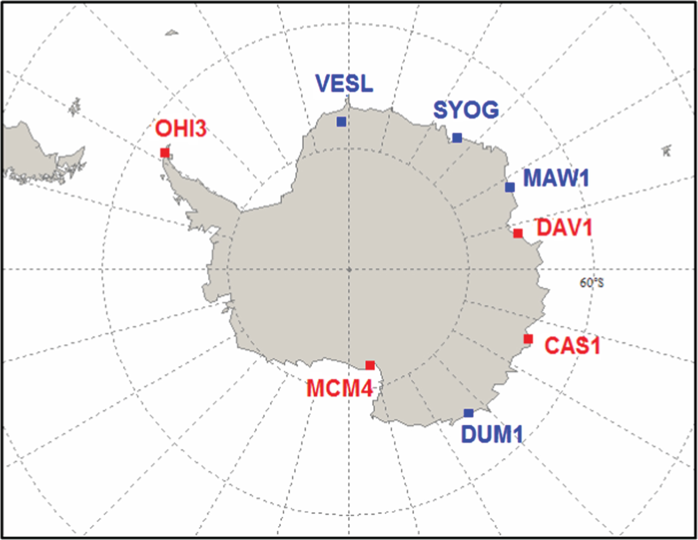
The data was collected from the Antarctica IGS network, which consists of eight stations (www.igs.org/network/). The distribution of the stations is shown in Figure 1. Four stations of the Multi-GNSS Experiment (MGEX) network (http://www.igs.org/mgex/) are marked in red. In this experiment, the data sets from these four MGEX stations on 19 December 2015 were investigated. The other four stations (marked in blue) were not used as they provide neither high-rate (1 Hz) nor multi-GNSS data. Table 1 shows the network baselines. We can see that the shortest baseline is more than 1,000 km; it is considered beyond the range of application for the DGPS technique, thus the DVA method is not involved in the computation in this experiment.

Figure 1. IGS station distribution over Antarctica. Four MGEX stations marked in red are used in this study. The other stations in blue are not involved in calculation as they collect neither high-rate (1 Hz) nor multi-GNSS data.

Table 1. Antarctica network data. These four stations are from Figure 1, with baseline length of thousands of kilometres.

4.2. Performance assessment of the NVA method using GPS data

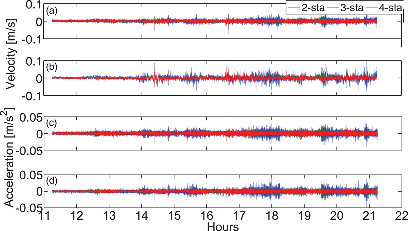
In this experiment, the data is taken from the IGS high-rate network with a one second sampling interval. DAV1 is regarded as the rover, CAS1 the master station, and MCM4 and OHI3 serve as the reference stations. Here we design three networks of different sizes, ranging from two to four stations. The LC and L1 observables are used to illustrate the effect of ionospheric drift on velocity and acceleration estimation. Results and statistics are shown in Figure 2 and Table 2.

Figure 2. Velocity ((a), (b)) and acceleration ((c), (d)) estimates by the NVA method with different networks and different types of observables. (a) and (c) are based on the LC observable, (b) and (d) are based on the L1 observable. The ionospheric drift may cause biased estimation of the velocity with L1 observable. Applying a three- or four-station network can generate more robust velocity and acceleration estimates than a two-station network.

Table 2. Statistics of velocity and acceleration estimates in the “Up” component as a function of network size with respect to DAV1. Master station CAS1 and the rover DAV1 are included in each network; the reference stations MCM4 and OHI3 are added to form the networks of size three and four.

With the increase of the number of stations, regardless of using the LC or L1 observable, the Root Mean Square (RMS) values of the velocity and acceleration estimates decrease. Compared to a two-station network, the improvement is significant when using a three-station network. Taking the LC observable as an example, the RMS values of the velocity and acceleration estimates improve by 32% and 31% in the “Up” component, respectively. This improvement is mainly due to the improved geometry, and the addition of one more reference station reinforces the estimation of satellite clock drifts. However, the improvement is not significant when using a four-station network compared to a three-station one. Thus, it is generally suggested to use a three-station network while applying the NVA method in Antarctica.

Figure 2 and Table 2 also show the effect of ionospheric drift on velocity and acceleration estimates. The results are comparable when using LC and L1 observables. Taking the four-station network for example, it can be seen that using LC leads to a decrease in dispersion (around 51% improvement in the average value) of velocity estimates compared to L1, while there is also a magnitude improvement in RMS of about 33% for the velocity estimates. This indicates that ionospheric drift may affect the velocity determination significantly over Antarctica. On the other hand, comparison of the RMS values of the acceleration estimates derived from the LC and L1 observables suggests that the ionospheric drift rate plays a minor role in the acceleration determination. Overall, for precise positioning, it is better to use LC for velocity and L1 for acceleration determination over Antarctica.

The NVA method-based velocity and acceleration estimates can be better than 5 mm/s and 3 mm/s²; the accuracy can still be improved if multi-GNSS observations are applied. That will be shown in the next experiment.

4.3. Performance assessment of the NVA and SVA methods using multi-GNSS data

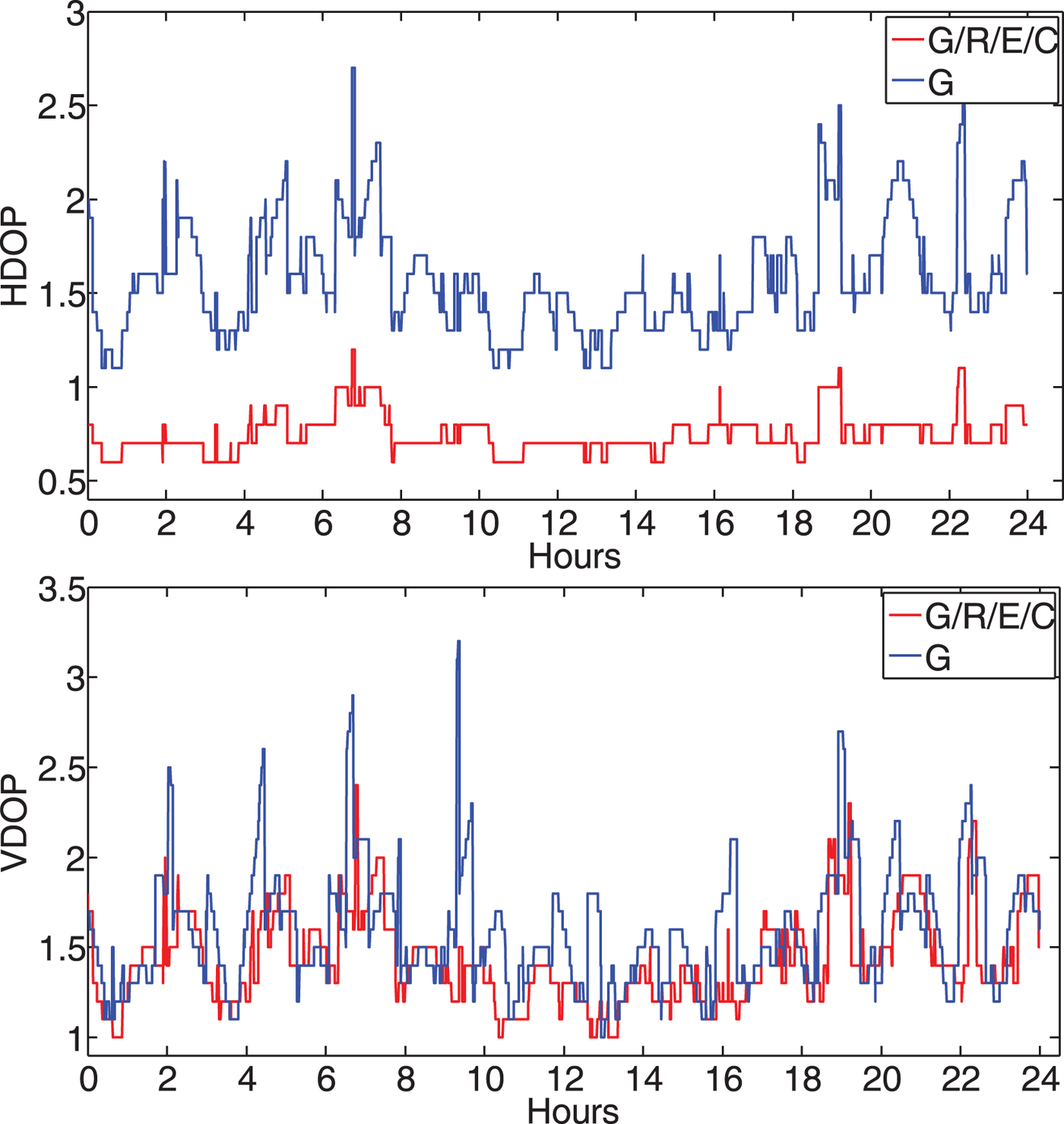
In this experiment, data was taken from the MGEX network with a sampling interval of 30 seconds. For the NVA method, the assignment of stations differed from the former test, with CAS1 as “rover”, MCM4 as “master” and DAV1 and OHI3 as “references”. This is because DAV1 collects only G/R data while CAS1, MCM4 and OHI3 all collect G/R/E/C data. For SVA, CAS1 was analysed in kinematic mode. Figure 3 shows the HDOP and VDOP values of station CAS1. It can be seen that, compared to a GPS-only system, the HDOP turns out to be much lower when using a G/R/E/C combined system. However, the VDOP does not improve significantly because of a lack of high elevation satellites over Antarctica.

Figure 3. HDOP and VDOP of station CAS1. The HDOP of the G/R/E/C combined system tends to be much lower than a GPS-only system because of the improved geometry, however the improvement is not significant for VDOP.

Effectiveness and reliability of multi-GNSS velocity and acceleration determination with the NVA and SVA methods are further compared and evaluated. For convenience, only the LC observable is calculated. The results are displayed in Figure 4 and Table 3. According to the analysis in Section 4.2, here we use a three-station network for the NVA method.

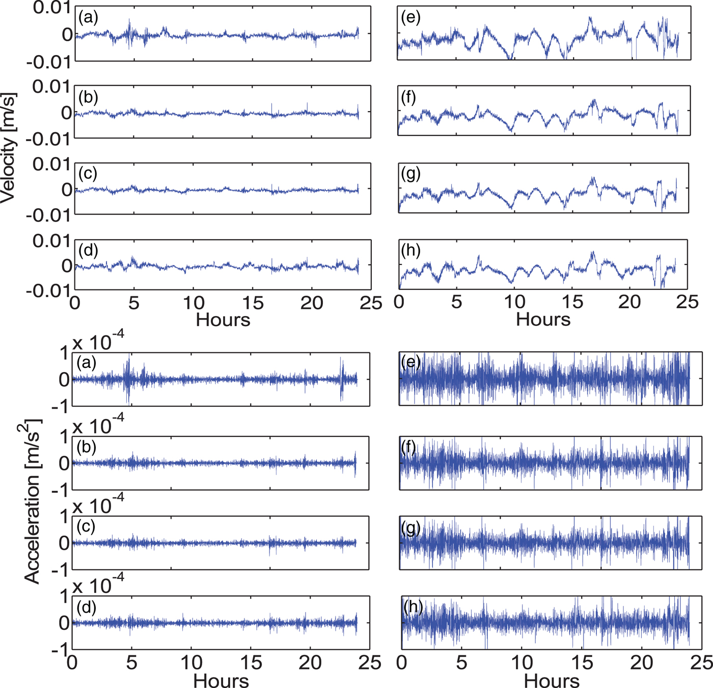
Figure 4. Velocity and acceleration estimates at 30 seconds interval by the NVA and SVA methods from application of different GNSS systems: G (a), G/R (b), G/R/E/C with PWR (c) and G/R/E/C with EWR (d), (e)–(h) are corresponding results from SVA. It clearly shows the higher performance of the NVA method with different systems.

Table 3. Statistics of velocity and acceleration estimates by the NVA and SVA methods using different GNSS systems.

For the two methods, the velocity and acceleration estimates using a G/R combined system are superior to those using a GPS-only system. The accuracy is improved by 25% and 29% for velocity and 37% and 31% for acceleration. However, the improvement is not significant when adding the Galileo and BeiDou systems. One reason is that the reference station DAV1 only observes G/R data. The other is that few Galileo and BeiDou satellites are observed (an average of three and six, respectively). The addition of Galileo and BeiDou satellites seems not to improve the VDOP of the G/R system. In addition, regarding the NVA method, the results from the PWR-based G/R/E/C combined system are superior to that from the EWR based-system. The posterior weight can effectively adjust the contributions of different systems and the accuracy is improved by 8% and 10% for velocity and acceleration, respectively. However, the RMS does not make a difference no matter what kind of weighting approach is applied for the SVA method. This is mainly because the accuracies of velocity or acceleration estimates by the SVA method are poor and even proper weighting does not make a significant improvement.

As the sampling interval is 30 seconds, compared with the experiment in Section 4.2 when using one second data, the measurement noise is suppressed by a magnitude of 30 when we conduct the epoch-differencing process. This is why the NVA-based velocity estimates have a much higher accuracy than with one second data, and RMS values of about 1 mm/s and 0·01 mm/s² for velocity and acceleration estimates can be obtained. However, when it comes to the SVA solution, there are obvious systematic errors in the velocity estimates. When considering the calculation process of the NVA and SVA solutions, the only difference is the derivation of the satellite clock drifts. As the satellite clock offsets are usually very stable or have a linear variation over a day, the derivation errors of the satellite clock offsets regarding one or 30 seconds should have the same magnitude and will be significant when the measurement noise is suppressed. It was found that the derivation errors may cause biased estimation of the velocity. However, for the NVA method, the satellite clock drift are estimated ‘on-the-fly’, which is still robust for velocity determination.

Overall, comparing the RMS values shown in Table 3, it can be seen that the NVA method is much more reliable than the SVA method when using 30 seconds data. It is thought that NVA using a network of stations can provide more robust satellite clock drift estimates, while SVA may be vulnerable to the derivation of the IGS clock products.

5. A REAL FLIGHT EXPERIMENT

An application of the NVA method to aircraft velocity and acceleration determination was tested. The data was recorded on the European Space Agency (ESA) PolarGap gravity field campaign, where a Twin-Otter aircraft was used (see Figure 5, left). The primary objective of this campaign was to perform an airborne gravity survey over the southern polar gap of the ESA's satellite gravity field mission GOCE (Gravity field and steady-state Ocean Circulation Explorer) (Jordan et al., Reference Jordan, Robinson, Olesen, Forsberg and Matsuoka2016). During the experiment, two reference stations called FD83-2 and FD83-3 were installed in a tented field camp FD83, the aircraft was parked next to FD83. The trajectory of this flight is shown in Figure 5, right. The aircraft took off from the camp, flew to the South Pole and then flew back to the camp. Besides the data from FD83-3 (FD83-2 was not used as it only observes GPS data), the GPS/GLONASS data from three IGS stations: OHI3, DAV1 and CAS1 (see Figure 1) were also used for NVA independent calculation purposes.

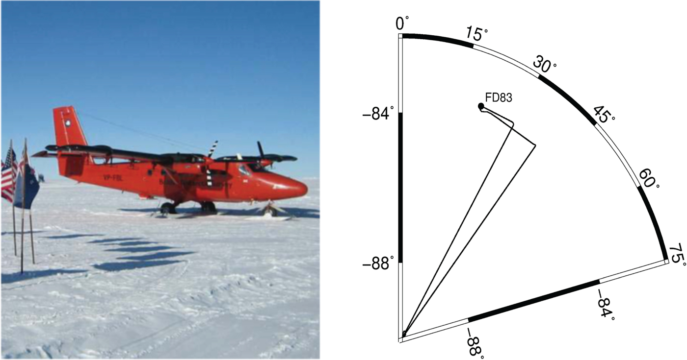
Figure 5. The Twin-Otter aircraft used in the ESA's PolarGap campaign (left) and the trajectory of this flight (right). The aircraft flew from the camp FD83 to the South Pole and then back to the camp.

Regarding the kinematic data collection process, two rover receivers named AIR1 and AIR2 were mounted on the aircraft. The flight was conducted on 19 December 2015. The duration of this flight was 10 h 50 min (from 10:30 to 21:20, local time). Here only AIR2 is involved in the calculation as it observed GPS and GLONASS data.

5.1. Aircraft data processing

For the three methods, the LC carrier phase observable was used for velocity and acceleration determination. Regarding the DVA method, FD83-3 is taken as the reference station. Its data processing was done with a software tool called HALO_GNSS (He et al., Reference He, Xu, Xu and Flechtner2016). When the aircraft was parked, it was quite close to FD83-3. However, when it flew, the distance between them (shown in Figure 6) became larger. After 14:00, it was more than 100 km and up to 750 km. The velocity estimates may be greatly affected by the common errors that are not eliminated by double-difference processing.

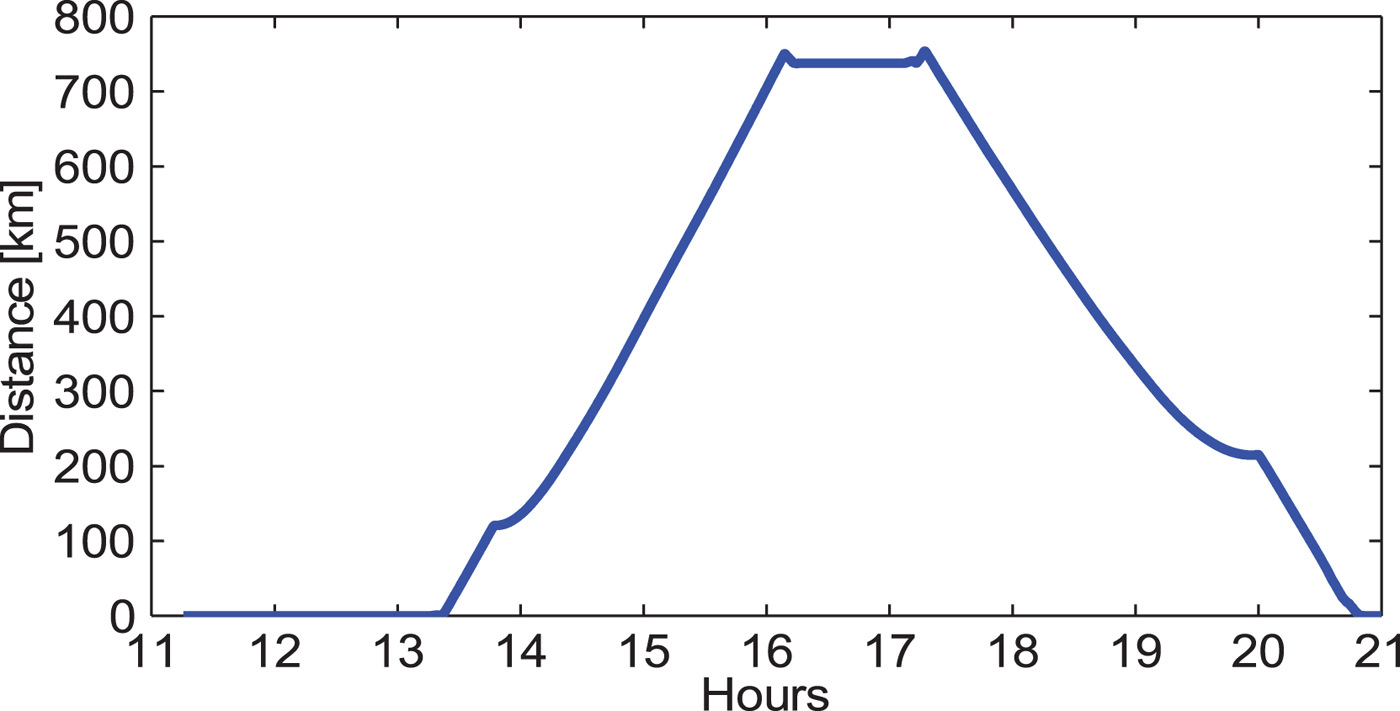
Figure 6. Distance between the rover and the reference station. The baseline can be as long as 700 km, which is a challenge for the application of the DVA method.

It is usually very difficult to establish a “reference solution” for a kinematic experiment. However, a better way to assess the results of each method is to study data from when the aircraft was parked next to the camp FD83, which was only 55 m from the reference station FD83-3. This period spanned from local time 10 h 30 min to 11 h 16 min. The results from the SVA and DVA methods were also calculated to make a comparison.

As Figure 7 shows, the vertical velocities obtained by the three methods are comparable when using a known zero reference solution during the static period. Table 4 presents a summary of the mean and RMS values of velocity and acceleration for the “Up” component during the static period. The RMS shows that the NVA method outperforms DVA and SVA in velocity estimation. It can produce velocity estimates with an accuracy of 3 mm/s or better. It also has better performance than the methods in Van Graas and Soloviev (Reference Van Graas and Soloviev2004) and Salazar et al. (Reference Salazar, Manuel, Jose, Jaume and Angela2011). This is because of the addition of the GLONASS observables. The acceleration estimates are similar, although the NVA method again shows slight advantages.

Figure 7. Vertical velocity and acceleration estimates during the static period.

Table 4. Statistics of vertical velocity and acceleration estimates for the NAV, SVA and DVA methods. It shows slight advantage of the NVA solution over the SVA and DVA solutions. Velocity of an accuracy of 3 mm/s can be obtained.

It is rather difficult to evaluate the kinematic results. Traditionally, the DGPS-based method is usually taken as an external assessment approach. For such a long range (0 ~ 750 km, see Figure 6), multiple reference stations that tend to have an increased number of common satellites are usually used, and it has already been successfully applied in many studies (Fotopoulos and Cannon, Reference Fotopoulos and Cannon2001; He et al., Reference He, Xu, Xu and Flechtner2016). However, in this contribution, only one reference station is used, although there is another reference station FD83-2, but they were mounted too close together and thus the kinematic solutions may not be enhanced by using a network of these two stations.

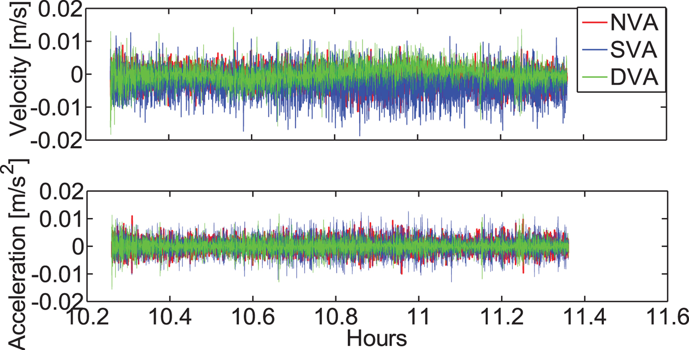
Instead, in order to evaluate the performances of the three methods, we compare differences among their velocity and acceleration estimates. Taking the velocity solutions for analysis, Figure 8 plots the velocity difference for the “Up” component during the period of the kinematic flight, Figure 8(a) and 8(b) are the differences between NVA and SVA with respect to DVA and Figure 8(c) is the difference between NVA and SVA. We can see larger biases in Figure 8(a) and 8(b) than in 8(c). The corresponding standard deviation values of velocity differences for Figure 8(a), 8(b) and 8(c) are 8·06, 7·98 and 4·88 mm/s, respectively. Such comparisons show that the NVA and SVA solutions agree with each other well while the DVA solution seems to be less consistent with the NVA or SVA solution. As in Least-Squares, usually the inner precision or the model accuracy can be evaluated by the post-fit RMS of the measurement residuals. Thus, the RMS of the velocity estimates of the three methods are calculated and their results are shown in Figure 8(d), 8(e) and 8(f). Starting at 14 h 30min, the distance is more than 200 km (see Figure 6). Differences become larger than shown in Figure 8(a) and 8(b) which is in accordance with the larger RMS shown in Figure 8(d). This demonstrates that with the increase of the distance between the rover and the reference station, the biases in velocity estimates of the DVA method also increase.

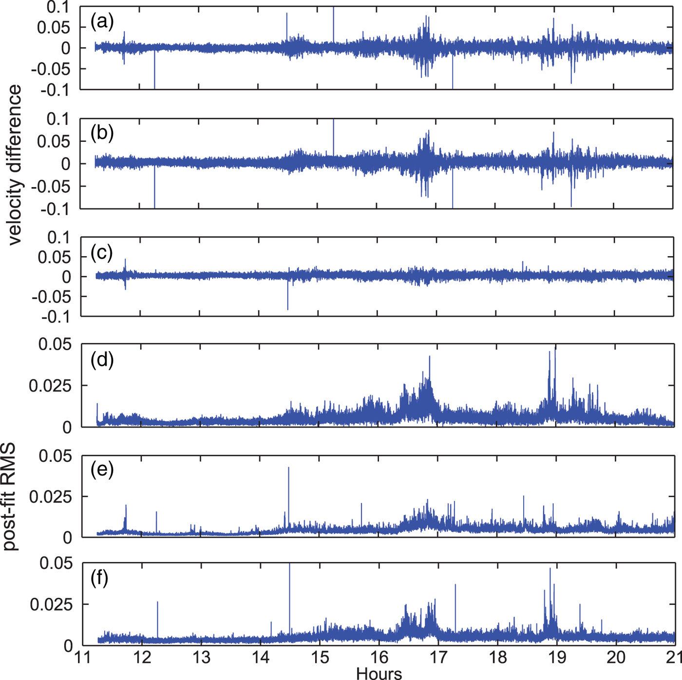
Figure 8. Aircraft velocity differences between NVA and DVA (a), SVA and DVA (b), NVA and SVA (c) during the kinematic flight period and epoch-by-epoch postfit RMS of DVA (d), NVA (e) and SVA (f) (unit: m/s). The NVA and SVA solutions seem to agree with each other well while the DVA solution may be biased with the increase of the baseline length.

It should be noted that the NVA and SVA solutions seem to be more consistent than the results in Section 4.3. That is mainly because here we use one second data and the magnitude of the two kinds of satellite clock drift errors are not significant compared to the epoch-differencing errors of measurements. The kinematic velocity estimates from the two methods still show differences with an STD of 4·88 mm/s, which suggests that satellite clock drifts from estimation ‘on-the-fly’ and by derivation may still cause difference to a notable extent in the velocity determination. As already demonstrated in the static test with 30 seconds data, the estimated satellite clock drifts tend to have a much lower noise, which is suggested for use in the kinematic velocity determination.

As the performance of acceleration is in accordance with velocity, overall, it can be concluded that for long range kinematic velocity and acceleration determination, the NVA method using a network of stations tends to be more robust and reliable than the single-baseline DGPS method.