1. INTRODUCTION
The pseudorange differential positioning technique was proposed some time ago. This technique can reduce the spatially correlated errors, such as tropospheric delay, ionospheric delay and satellite orbit errors, and therefore improves positioning accuracy compared with single point positioning. The process procedure is simple because it does not need to handle integer ambiguity, which is a difficult and crucial problem in carrier-phase positioning. As a result, it has been widely used in coastal navigation, vehicle navigation, aircraft landing and other fields.
Many researchers have contributed to the Global Positioning System (GPS) pseudorange differential positioning technique. Basic principles, algorithm implementation, and applications can be found in Teasley et al. (Reference Teasley, Hoover and Johnson1980), Kalafus et al. (Reference Kalafus, Vilcans and Knable1983), Blackwell (Reference Blackwell1985), and Morgan-Owen and Johnston (Reference Morgan-Owen and Johnston1995). Positioning performance under the Selective Availability policy was analysed by Beser and Parkinson (Reference Beser and Parkinson1982). Hatch (Reference Hatch1982) presented the single-frequency phase-smoothed pseudorange method, which was known as the Hatch filter. In order to reduce the influence of ionospheric divergence, dual-frequency GPS data was used to improve the accuracy of phase-smoothed pseudorange measurements by Hwang et al. (Reference Hwang, Mcgraw and Bader1999). The positioning performance in different scenarios was discussed in Vallot et al. (Reference Vallot, Snyder, Schipper, Parker and Spitzer1991), Pikander and Eskilinen (Reference Pikander and Eskelinen2004), Huang and Tan (Reference Huang and Tan2006), and Matosevic et al. (Reference Matosevic, Salcic and Berber2006).
The BeiDou Navigation Satellite System (BDS) had successfully launched 16 satellites by the end of 2012, and begun to provide regional services in the Asia-Pacific region. According to the officially published BDS Open Service Performance Specification (China Satellite Navigation Office, 2013) on 27 December 2013, the horizontal and vertical positioning accuracy are both better than 10 m (95 % confidence level). The performance of BDS pseudorange differential positioning and single point positioning were compared in Liu and Yang (Reference Liu and Yang2011). They found that the former are more reliable than the latter. Chen et al. (Reference Chen, Gao and Wu2012) demonstrated that combined GPS/BDS pseudorange differential positioning shows better performance than a single system when the observation environment is poor. Since phase smoothing with ionosphere-free combination would amplify the noise and multipath, Xu et al. (Reference Xu, Li, He, Guo and Wang2014) discussed different linear combinations for BDS phase-smoothed pseudorange differential positioning. In this paper, a study on BDS phase-smoothed pseudorange differential positioning using different frequency signals and different length baselines is introduced.
Basic principles of BDS pseudorange differential positioning and a dual-frequency phase smoothing formula considering the ionospheric delay are introduced in Section 2. In Section 3, the BDS and GPS observation data from Hubei CORS (Continuously Operating Reference System) and Bohai Bay RBN-DGNSS (Radio Beacon-Differential Global Navigation Satellite System) testing net in China were collected, the phase-smoothed pseudorange observables of GPS L1, BDS B1, and BDS B3 signals were applied, and the pseudorange corrections were generated at the base stations. Then we applied the pseudorange differential positioning technique at the roving stations. Finally, we made a comparison of the positioning performance using smoothed BDS B1, B3, and GPS L1 pseudoranges respectively. The relation between the positioning accuracy and the baseline length was also analysed.
2. BASIC PRINCIPLES OF PHASE-SMOOTHED PSEUDORANGE DIFFERENTIAL POSITIONING
2.1. Pseudorange differential positioning
2.1.1. Basic theory
The basic theory includes the method of generating the pseudorange corrections, and the functional and stochastic models used for the pseudorange differential positioning.
The corrections of pseudorange at a base station can be expressed as (Hofmann-Wellenhof et al., Reference Hofmann-Wellenhof, Lichtenegger and Wasle2008),
 $$\Delta P_b^q = R_b^q - P_b^q = c\delta {\tau _b} - c\delta {\tau ^q} + \delta O_b^q + \delta T_b^q + \delta I_b^q $$
where the subscript b and the superscript q represent the receiver and the satellite respectively, R denotes the distance between the station and the satellite, P is the original pseudorange observable. c stands for the speed of light, δτ b and δτ q represent the receiver's and the satellite's clock error respectively. δO is the orbit error, and δI and δT are the ionospheric and tropospheric delay respectively.
For a roving station, the pseudorange between satellite q and station r can be measured at the same time. If the roving station can synchronously obtain the correction of the base station via a communication network, the measured pseudorange of the roving station can be corrected, as follows,
 $$\eqalign{P_{r,corr}^q & = P_r^q + \Delta P_b^q = R_r^q - c(\delta {\tau _r} - \delta {\tau _b}) - (\delta O_r^q - \delta O_b^q ) \cr &\quad - (\delta I_r^q - \delta I_b^q ) - (\delta T_r^q - \delta T_b^q )}$$
where the subscript r denotes the receiver. Provided that the distance between the base and roving station is short, the orbit errors, the ionospheric and the tropospheric delays at the base station and the roving station are approximately identical. Therefore, the corresponding terms of the above equation can be removed and the equation becomes:
 $$\eqalign{P_{r,corr}^q & = P_r^q + \Delta P_b^q = R_r^q - c(\delta {\tau _r} - \delta {\tau _b}) \cr & = \sqrt {{{({X^q} - {X_r})}^2} + {{({Y^q} - {Y_r})}^2} + {{({Z^q} - {Z_r})}^2}} - c(\delta {\tau _r} - \delta {\tau _b})}$$
The linearized corrected pseudorange observation equation is expressed as
 $$P_{r,corr}^q = - l_r^q dX - m_r^q dY - n_r^q dZ - c(\delta {\tau _r} - \delta {\tau _b}) + R_r^q $$
where the symbols l, m and n are the unit vector on the line-of-sight from the receiver r to the satellite q. The coordinate correction components dX, dY and dZ, and the relative receiver clock error are to be solved.
Suppose that the Standard Deviations (STD) of the corrected pseudorange observations for each satellite are the same, which are σ P , and a prior standard deviation σ 0 is equal to σ P . Considering the influence of satellite elevations on STD determination, the variance of the observation at the roving station observing satellite q at satellite elevation ele can be expressed as
 $${\left( {\sigma _r^q} \right)^2}(ele) = \left\{ {\matrix{ {\sigma _P^2 \cdot {{\csc} ^2}\left( {ele} \right),} & {ele \lt {{30}^ \circ}} \cr {\sigma _P^2 \cdot \csc \left( {ele} \right),} & {ele \ge {{30}^ \circ}} \cr}} \right.$$
then the corresponding weight matrices in the corrected pseudorange observation equation are
 $${\rm \bf P} = \sigma _0^2 {{\rm \bf D}^{ - 1}} = \sigma _0^2 \left[ {\matrix{ {\displaystyle{1 \over {{{\left( {\sigma _r^1} \right)}^2}}}} & 0 & \cdots & 0 \cr 0 & {\displaystyle{1 \over {{{\left( {\sigma _r^2} \right)}^2}}}} & \cdots & 0 \cr \vdots & \vdots & \ddots & \vdots \cr 0 & 0 & \cdots & {\displaystyle{1 \over {{{\left( {\sigma _r^s} \right)}^2}}}} \cr}} \right]$$
where s is the total visible satellite number at the present epoch, which should not be less than four. It can be clearly found that the weight matrices only depend on the satellite elevations.
2.1.2. BDS IODE determination method
The basic theory of BDS pseudorange differential positioning is similar to that of GPS, which has been introduced above. However, there is a distinction between BDS and GPS.
The roving station will use the pseudorange corrections transmitted from the base station if the IODE (Issue of Data Ephemerides) of the two stations are equal, which means the roving and the base stations use the identical version of the ephemeris. The GPS IODE varies with the time, while the BDS IODE is a constant value (it is 1 in the experiment data). So we cannot use BDS IODE for time matching of the corrections.
Based on the above, a generation method for BDS IODE (ranging from 0 to 252) is proposed. Since the TOE (Time of Ephemeris, ranging from 0 to 604800) is different from each other during one week, a mapping function of TOE can be adopted to determine the IODE, as follows,
 $${\rm IODE} = \left\{ {\matrix{ {{\mathop{\rm int}} ({\rm TOE}/1200),} \hfill & {0 \le {\rm TOE} \le 302400} \hfill \cr {{\mathop{\rm int}} (({\rm TOE} - 302400)/1200),} \hfill & {302400 \lt {\rm TOE} \lt 604800} \hfill \cr}} \right.$$
where int is the rounding symbol. The above function can make sure that the BDS IODE are different at two adjacent moments (a BDS satellite will change its ephemeris at one hour intervals). Then the IODE calculated from Equation (7) can be used for BDS pseudorange differential positioning.
2.2. Dual-frequency phase-smoothed pseudorange
The phase-smoothed pseudorange algorithm is generally referred to as the Hatch filter (Hatch, Reference Hatch1982). However, strictly speaking, the Hatch filter estimator is not a recursive least-squares estimator, see Teunissen (Reference Teunissen1991). The phase-smoothed pseudorange estimator is very close to optimal only in the case of the absence of satellite redundancy. Instead, the proposed phase-adjusted pseudorange estimator, which is proved to be the optimal, has been widely used in precise point positioning (Le and Teunissen, Reference Le and Teunissen2006; Le and Tiberius, Reference Le and Tiberius2006). However, the error models used in pseudorange differential positioning cannot satisfy the accuracy requirement of ambiguity resolution in the phase-adjusted pseudorange model, so the above method cannot perform well in pseudorange differential positioning. Therefore, the Hatch filter is still the most popular approach in pseudorange differential positioning owing to its simple operability. The dual-frequency phase-smoothed pseudorange algorithm applied in this paper is based on the Hatch filter.
By differencing the dual-frequency pseudorange and carrier-phase observables at two adjacent epochs (e.g. t k and t k+1) and supposing that there is no cycle slip in the observation, we can yield,
 $$\Delta {P_i}({t_k},{t_{k + 1}}) = \Delta \rho ({t_k},{t_{k + 1}}) + \Delta {I_i}({t_k},{t_{k + 1}}) + \Delta {\varepsilon _{Pi}}({t_k},{t_{k + 1}})$$
 $$\Delta {P_j}({t_k},{t_{k + 1}}) = \Delta \rho ({t_k},{t_{k + 1}}) + \gamma \Delta {I_i}({t_k},{t_{k + 1}}) + \Delta {\varepsilon _{Pj}}({t_k},{t_{k + 1}})$$
 $$\Delta {L_i}({t_k},{t_{k + 1}}) = \Delta \rho ({t_k},{t_{k + 1}}) - \Delta {I_i}({t_k},{t_{k + 1}}) + \Delta {\varepsilon _{Li}}({t_k},{t_{k + 1}})$$
 $$\Delta {L_j}({t_k},{t_{k + 1}}) = \Delta \rho ({t_k},{t_{k + 1}}) - \gamma \Delta {I_i}({t_k},{t_{k + 1}}) + \Delta {\varepsilon _{Lj}}({t_k},{t_{k + 1}})$$
where P is the pseudorange observable, L is the carrier phase observable in units of metres, the subscript number i and j denote the signals of L1 and L2 for GPS, and B1 and B3 for BDS. ρ is the frequency-free term including the distance between the receiver and the satellite, the orbit error and the tropospheric delay. I is the ionospheric delay, γ is the ratio of the square of frequency i and the square of frequency j (
 ${\rm \gamma} = \displaystyle{{f_1^2} \over {f_2^2}} $
for GPS, and
${\rm \gamma} = \displaystyle{{f_1^2} \over {f_2^2}} $
for GPS, and
 ${\rm \gamma} = \displaystyle{{f_1^2} \over {f_3^2}} $
for BDS in this paper), and the last term ε is the observation noise. Considering the similar code rate (2·046 Mcps) and observation noise level of B1 and B2 signals, only B1 signal is used to compare to B3 signal. Substitute Equation (8) and (9) into Equations (10) and (11) to remove the distance variation Δρ, and we can get the predicted pseudorange, which is expressed as follows:
${\rm \gamma} = \displaystyle{{f_1^2} \over {f_3^2}} $
for BDS in this paper), and the last term ε is the observation noise. Considering the similar code rate (2·046 Mcps) and observation noise level of B1 and B2 signals, only B1 signal is used to compare to B3 signal. Substitute Equation (8) and (9) into Equations (10) and (11) to remove the distance variation Δρ, and we can get the predicted pseudorange, which is expressed as follows:
 $${{\breve P} _i}({t_{k,k + 1}}) = {{\breve P} _i}({t_k}) + \Delta {L_i}({t_k},{t_{k + 1}}) + 2\Delta {I_i}({t_k},{t_{k + 1}})$$
 $${{{\breve P}} _j}({t_{k,k + 1}}) = {{\breve P} _j}({t_k}) + \Delta {L_j}({t_k},{t_{k + 1}}) + 2\gamma \Delta {I_i}({t_k},{t_{k + 1}})$$
For single-frequency observables, the variation of the ionospheric delay between two adjacent epochs ΔI i (t k , t k+1) is hard to determine. Although there are many ionosphere models available, such as the Klobuchar model and Global Ionosphere Map (GIM), those models are not used in pseudorange differential positioning due to various reasons. The ionospheric correction parameters for BDS are not provided yet, so we cannot compute the ionospheric delay by the Klobuchar model. The GIM products need to be downloaded from the internet, which would increase the communication burden. Considering the fact that the ionospheric delay usually changes gradually, the variation is very small and is regarded as zero within an appropriate window length. A simple window length is applied to the traditional Hatch filter for the limitation of the smoothing divergence. After the Hatch filter, the smoothed pseudorange is a weighted combination of the original pseudorange and the predicted pseudorange, which can be expressed as
 $${\breve P} ({t_{k + 1}}) = \displaystyle{{P({t_{k + 1}})} \over {k + 1}} + \displaystyle{k \over {k + 1}}{\breve P} ({t_{{k},\,{k + 1}}}) = \displaystyle{{P({t_{k + 1}})} \over {k + 1}} + \displaystyle{k \over {k + 1}}[{\breve P} ({t_k}) + \Delta L({t_k},{t_{k + 1}})]$$
where k is the epoch number in the filter and the initial smoothed pseudorange is the original observable.
However, if the ionospheric delay is dramatically changed at some time, or the variation has accumulated to a relatively large value as the time goes by (i.e. the window length may be not appropriate), the filter will be divergent and lead to an incorrect result.
To avoid the divergence caused by the variation of the ionospheric delay, dual-frequency observables are used to eliminate the ionospheric delay. From Equations (10) and (11), we can get
 $$\Delta {I_i}({t_k},{t_{k + 1}}) = \displaystyle{1 \over {\gamma - 1}}\left[ {\Delta {L_i}({t_k},{t_{k + 1}}) - \Delta {L_j}({t_k},{t_{k + 1}})} \right]$$
Substituting Equation (15) into Equations (12) and (13), we can obtain the modified Hatch filter formula, as follows,
 $$\left\{ {\matrix{ {{{{\breve P}} _i}({t_{k + 1}}) = \displaystyle{{{P_i}({t_{k + 1}})} \over {k + 1}} + \displaystyle{k \over {k + 1}}\left[ {{{{\breve P}} _i}({t_k}) + \Delta {L_i}({t_k},{t_{k + 1}}) + \displaystyle{2 \over {\gamma - 1}}\left[ {\Delta {L_i}({t_k},{t_{k + 1}}) - \Delta {L_j}({t_k},{t_{k + 1}})} \right]} \right]} \cr {{{{\breve P}} _j}({t_{k + 1}}) = \displaystyle{{{P_j}({t_{k + 1}})} \over {k + 1}} + \displaystyle{k \over {k + 1}}\left[ {{{{\breve P}} _j}({t_k}) + \Delta {L_j}({t_k},{t_{k + 1}}) + \displaystyle{{2\gamma} \over {\gamma - 1}}\left[ {\Delta {L_i}({t_k},{t_{k + 1}}) - \Delta {L_j}({t_k},{t_{k + 1}})} \right]} \right]} \cr}} \right.$$
Generally speaking, there is no correlation between the code pseudorange and the carrier-phase observations whether the frequencies are the same or not (Bona, Reference Bona2000), while the carrier-phase measurements are cross-correlated with a cross correlation coefficient of about 0·3–0·4. We assume that the standard deviations of code pseudorange and carrier-phase observations are σP1 = σP3 = 0·3 m, and σL1 = σL3 = 0·003 m respectively for BDS B1 and B3 signals, and the correlation coefficient of carrier-phase observations is 0·4. Then we can get the covariance of B1 and B3 carrier-phase observations, i.e. δ = 0·0000036 m. Assuming no time correlation between code pseudorange and carrier-phase observations, an application of propagation law of covariances to Equation (16) gives,
 $$\left\{ {\matrix{ {\sigma _{{P_1},{t_{k + 1}}}^2 = \displaystyle{{\sigma _{{P_1}}^2 + k\left[ {{{\left( {\displaystyle{{\gamma + 1} \over {\gamma - 1}}} \right)}^2}\sigma _{{L_1}}^2 + \displaystyle{4 \over {{{\left( {\gamma - 1} \right)}^2}}}\sigma _{{L_3}}^2 - \displaystyle{{4\left( {\gamma + 1} \right)} \over {\gamma - 1}}\delta} \right]} \over {k + 1}} = \displaystyle{{\sigma _{{P_1}}^2 + k\sigma _1^2} \over {k + 1}}} \cr {\sigma _{{P_3},{t_{k + 1}}}^2 = \displaystyle{{\sigma _{{P_3}}^2 + k\left[ {{{\left( {\displaystyle{{3\gamma - 1} \over {\gamma - 1}}} \right)}^2}\sigma _{{L_1}}^2 + \displaystyle{{4{\gamma ^2}} \over {{{\left( {\gamma - 1} \right)}^2}}}\sigma _{{L_3}}^2 - \displaystyle{{4\gamma \left( {3\gamma + 1} \right)} \over {\gamma - 1}}\delta} \right]} \over {k + 1}} = \displaystyle{{\sigma _{{P_3}}^2 + k\sigma _3^2} \over {k + 1}}} \cr}} \right.$$
Then the values of
 $\sigma _1^2 $
and
$\sigma _1^2 $
and
 $\sigma _3^2 $
can be obtained, i.e.
$\sigma _3^2 $
can be obtained, i.e.
 $\sigma _1^2 = 0\cdot0007\,{{\rm m}^2}$
and
$\sigma _1^2 = 0\cdot0007\,{{\rm m}^2}$
and
 $\sigma _3^2 = 0\cdot0006\,{{\rm m}^2}$
, which are still far less than that of code pseudorange. The GPS dual-frequency smoothing has a similar result. The overall accuracy of dual-frequency smoothed pseudorange is higher than that of single-frequency smoothed pseudorange resulting from the elimination of ionospheric variation, though the noise of the smoothed pseudorange has been amplified. Also, the influences of the dual-frequency carrier-phase observations on different single-frequency pseudoranges in the modified Hatch filter are almost equal.
$\sigma _3^2 = 0\cdot0006\,{{\rm m}^2}$
, which are still far less than that of code pseudorange. The GPS dual-frequency smoothing has a similar result. The overall accuracy of dual-frequency smoothed pseudorange is higher than that of single-frequency smoothed pseudorange resulting from the elimination of ionospheric variation, though the noise of the smoothed pseudorange has been amplified. Also, the influences of the dual-frequency carrier-phase observations on different single-frequency pseudoranges in the modified Hatch filter are almost equal.
3. EXPERIMENT AND RESULT ANALYSIS
3.1. Data description
Two groups of BDS/GPS baseline data were collected in Hubei CORS and Bohai Bay RBN-DGNSS testing net. The UR370 and PBD25 receivers, manufactured by the Unicore and ComNav Companies of China respectively, were equipped for two groups respectively. Table 1 gives a summary of the two data groups, including the distance between the base and the roving stations, the observation dates, the observation durations, the sampling rates, and the observation locations. The Bernese 5·0 software was employed to obtain the precise coordinates of the base and the roving stations, which will be treated as the true values.
Table 1. Receiver Data.

The GPS L1, L2 and BDS B1, B3 signals are used for the modified Hatch filter, and the cycle slips were detected using both the MW combination (L6) and the geometry-free combination (L4) (Blewitt, Reference Blewitt1990). The precise smoothed pseudoranges were achieved thereby, and they were processed in the subsequent pseudorange differential positioning.
3.2. Processing results
Pseudorange differential positioning using smoothed BDS B1, B3, or GPS L1 pseudoranges is employed for the selected stations and the position deviations in different directions (north, east and vertical) are shown in Figure 1. It can be seen that the position deviations in the north, east and vertical directions fluctuate over the observation times. The position deviations in the horizontal component are more stable than those in the vertical component for signals of all three different frequencies. The position deviations in the horizontal component for BDS B1 and B3 signals have a slight difference from those for the GPS L1 signal, while their deviations in the vertical component are quite different. The largest bias for BDS B1 and B3 signals can be up to 6 m, which is nearly three times larger than that for GPS L1 signal.

Figure 1. Position deviations in north (N), east (E), and vertical (V) directions for Group A (left) and Group B (right).
The position deviations in Figure 1 (b) are more stable than those in Figure 1 (a). The baseline data of Group B were observed in 2014, while the data of Group A were observed in 2013 during the unstable period of the BDS system, and the PBD25 receivers used for Group B perform better than the UR370 receivers used for Group A. In addition, the small sample rate is also an advantage for Group B. The better positioning result can be seen in the right column sub-figures (Group B) in Figure 1.
It should be pointed out that outliers exist for Baseline IV and VIII. They lead to much larger position deviations and then the results are discarded, which is shown by four grey circles in the bottom two subfigures. In addition, the mean square error of a point at the outlier epoch is much larger than 3 m.
If a cycle slip occurs, the smoothing procedure will be re-initialised, which will immediately result in poor smoothing accuracy, and the positioning accuracy will be abruptly reduced. The apparent two re-initialisations are shown by two orange circles for Baseline V and VI. Since the receiver performs better for GPS than for BDS and more cycle slips exist in BDS carrier-phase observables, the stability of positioning deviations for BDS is worse than GPS, as we can see in Figure 1.
3.3. Results analysis
Three different strategies of statistical analysis are employed in this paper, which are used to evaluate the accuracy of phase-smoothed pseudorange differential positioning for BDS B1, B3, and GPS L1 signals.
3.3.1. The first strategy
The first accuracy evaluation index is the Root Mean Square (RMS) of the position deviations, which can be defined as follows,
 $$RMS = \displaystyle{{\sqrt {\sum\limits_{i = 1}^n {dev_i^2}}} \over n}$$
where i means the i-th epoch, n is the total valid epoch number, and dev is the position deviations for BDS B1, B3, or GPS L1 signals. Herein the “valid epoch” is defined as the mean square error of a point in this epoch is no larger than 5 m. Obviously, the smaller the RMS value is, the higher the accuracy. The percentage of valid epochs with respect to the whole number of epochs is given in Table 2. It can be seen that the number of valid epochs reaches up to 90% of the whole number of epochs.
Table 2. The percentage of valid epochs with respect to the whole number of epochs.

Table 3 describes the RMS of the position deviations for both baseline groups. It can be seen that the RMS values for all three signals are smaller than 2 m in the horizontal component, and 3 m in the vertical component, even with a distance of nearly 300 km. This level of accuracy can satisfy the requirement of RBN-DGNSS, whose horizontal accuracy should be below 5 m.
Table 3. The RMS of the position deviations in horizontal (H) and vertical (V) components for different signals and different baselines.

As to Group A, the RMS for BDS B3 signal is much larger than that for the GPS L1 signal in both horizontal and vertical components, though it is a little smaller than that for the BDS B1 signal. The RMS in both horizontal and vertical components has a gradual rising trend as the baseline length increases for all three signals. However, the RMS differences between different signals decrease, especially for the difference between BDS B1 and B3 signals.
The RMS differences between BDS B1/B3 and GPS L1 signals are not significant for Group B, especially in the horizontal component. The RMS for BDS B1/B3 signals is less than 2 m in both horizontal and vertical components. Since the BDS system becomes more stable after early 2014, the RMS for BDS B1/B3 signals gets close to that for the GPS L1 signal in both horizontal and vertical components for Group B. The rising trend of RMS for all three signals for Group B is not obvious, which partly results from the better performance of the receivers.
3.3.2. The second strategy
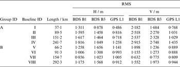
In the second strategy, the accuracy under the 95% confidence level is adopted. The deviations are ranked from the smallest value to the largest value, and the deviations in the first 95% epochs are chosen as the corresponding accuracy.
The accuracy under the 95% confidence level in the horizontal and vertical components for both BDS B1/B3, and GPS L1 signals are given in Table 4. We can see that the positioning accuracy of BDS B1/B3 signals for Group A is decreasing dramatically as the baseline length increases, which can reach up to 3 m and 6 m in horizontal and vertical components for a long baseline (>200 km).
Table 4. Accuracy under the 95 % confidence level in horizontal (H) and vertical (V) components for different signals and different baselines.

The positioning accuracy in the horizontal component of BDS B1/B3 signals for Group B fluctuates stably when baseline length is shorter than 200 km, while the corresponding accuracy in vertical component of B1 signal varies dramatically. However, when the distance between the base and the roving stations is longer than 200 km, the positioning accuracy of BDS B1/B3 signals plummets to 2 m and 3 m in horizontal and vertical components.
The positioning accuracy in both horizontal and vertical components for GPS L1 and BDS B1/B3 signals in Group B is better than that in Group A, especially for BDS B1/B3 signals. The positioning accuracy for the GPS L1 signal is better than that for BDS B1/B3 signals for both groups, especially in the vertical component.
3.3.3. The third strategy
The percentage of the position deviations under a given threshold is proposed as another index to assess the positioning accuracy in the third strategy. The thresholds are set as 1·5 m and 3 m in the horizontal component, and 2·5 m and 5 m in the vertical component separately, and then the corresponding percentage can be yielded from statistics.
Table 5 gives the statistical percentages of the position deviations under the pre-set criteria for GPS L1, BDS B1 and B3 signals. It is observed that the percentages of the position deviations less than 3 m in the horizontal component and 5 m in the vertical component for B3 and B1 signals can reach up to 90%. The statistical results for the GPS L1 signal are obviously superior to those for BDS signals, especially for long baselines (>200 km).
Table 5. Statistical table of the position deviations in each threshold.

As to Group A, the percentages of the position deviations less than 1·5 m in the horizontal component and 2·5 m in the vertical component for BDS B1/B3 signals can reach up to 50%. The percentages of the position deviations for BDS B1/B3 signals in almost all scenarios are remarkably lower than those for the GPS L1 signal.
The percentages of the position deviations less than 3 m and 5 m in horizontal and vertical components for both B1 and B3 signals can reach up to 99% for Group B, while the percentages of the position deviations less than 1·5 m and 2·5 m in horizontal and vertical components for B1 and B3 signals are markedly different. The percentages of the position deviations less than 1·5 m and 2·5 m in horizontal and vertical components for the B3 signal are sometimes significantly smaller than those for the B1 signal. Therefore, compared with the position accuracy of the B1 signal, BDS B3 single-frequency pseudorange differential positioning results are precarious.
3.4. Discussion
The analysed results by all three strategies are given in Figure 2. It can be seen that the positioning accuracy for BDS B1, B3, and GPS L1 signals experience a similar declining trend as the baseline length increases, while the positioning accuracy of Group B does not decline significantly. Since some electromagnetic interferences exist during the observation of Baseline V, the BDS positioning accuracy of Baseline V gets worse, as can be seen in the right column subfigures. The positioning results show a downward trend in Group B when removing Baseline V. In all three strategies, the positioning accuracy for GPS is higher than that for BDS, especially in the vertical component for long baselines (>200 km).

Figure 2. The statistical results of the three strategies for Group A (left) and Group B (right). The top row shows the RMS of the position deviations, the middle row shows the accuracy under the 95 % confidence level, and the bottom two rows show the results of the third strategy.
The positioning accuracy for the B3 signal is of similar magnitude to that for the B1 signal for short baselines (⩽200 km) but this situation is changed for long baselines. When the baseline length gets longer, the positioning accuracy decline rate for the B3 signal is remarkably faster than that for the B1 signal, especially for Group B. As the baseline distance increases, the difference of the ionosphere delay for different frequencies’ signals becomes larger and larger, and they should be taken into account, and will even replace the pseudorange multipath and measurement noise to become the crucial factors in making a difference to positioning accuracy for long baseline positioning. Considering the frequency of B3 (1,268·520 MHz) is smaller than that of B1 (1,561·098 MHz), the ionosphere delay of B3 signal will be larger and offset the smaller noise for the same long distance. Consequently, the difference of positioning accuracy for B1 and B3 signals is smaller, and finally the positioning accuracy of BDS B3 signal will be worse than that of the BDS B1 signal.
4. CONCLUSIONS
In this work, we reviewed the theoretical basis of the pseudorange differential positioning model and dual-frequency phase-smoothed pseudorange technique, introduced the modified Hatch filter, and then demonstrated the performance of pseudorange differential positioning using BDS B1, B3 and GPS L1 signals whose observations are smoothed by a modified Hatch filter. From the perspective of the positioning accuracy of our experiments we can draw some conclusions, which are listed as follows:
-
1) The longer the baseline length is, the worse the positioning accuracy gets, no matter whether for GPS L1 signal or for BDS B1 and B3 signals because of the decline of the spatial correlation of errors. Also, the positioning accuracy decline rate for the BDS signal is significantly faster than that of GPS signals for long baselines (>200 km), furthermore, the corresponding rate for the B3 signal is faster than that for the B1 signal.
-
2) GPS L1 signal performs better than BDS B1 and B3 signals in phase-smoothed pseudorange differential positioning, and its positioning deviations are much smaller, especially in the vertical component.
-
3) Generally speaking, the positioning accuracy of phase-smoothed pseudorange differential positioning for BDS can be up to 2 m (RMS) in the horizontal component, and 3 m (RMS) in the vertical component. In practice, the corresponding accuracy is better than 3·5 m and 7 m under a confidence level of 95 %. And the BDS signal can be used for the RBN-DGNSS application due to its competent positioning accuracy.
-
4) The positioning accuracy of BDS B1 and B3 signals is partly influenced by the system stability, the receivers on the base and the roving stations, and the sample rate.
ACKNOWLEDGEMENTS
This work is sponsored by National 863 project of China (2014AA123101/01). We are very grateful to Ms. L. Jin and Mr. K. Xu in Wuhan University, for their drawing guidance. We also thank the anonymous reviewers very much for their constructive comments and suggestions.