1. INTRODUCTION
Pulsars are highly magnetised rotating neutron stars, emitting electromagnetic radiation along their magnetic field axis. As the star rotates about its spin axis, the radiation appears to emit pulses towards an observer as the magnetic pole sweeps past the observer's line of sight to the star. These pulses are characterised by extremely strong stability and regularity to such an extent that their periodic accuracy compares well with today's atomic clocks (Mitchell et al., Reference Mitchell, Hassouneh, Wintemitz, Valdez, Price, Semper, Yu, Arzoumanian, Ray, Wood, Litchford and Gendreau2015; Zhang et al., Reference Zhang, Shuai, Huang, Chen and Xu2017; Ning et al., Reference Ning, Yang, Gui, Wu, Fang and Liu2018). This feature makes pulsars good candidates to be employed by navigation systems. X-ray Pulsar Navigation (XPNAV), which makes use of the X-ray radiation of pulsars, has been investigated (Sheikh, Reference Sheikh2005; Shiekh et al., Reference Sheikh, Golshan and Pines2007; Ma et al., Reference Ma, Wang, Jiang, Mu and Baoyin2017; Guo et al., Reference Guo, Sun, Hu and Xue2018). Compared with traditional celestial navigation methods, XPNAV can provide a whole navigation solution consisting of time, position, velocity and attitude, and can provide a seamless navigation service for spacecraft flying from near-Earth orbit to deep space (Backer et al., 2018; Chen et al., Reference Chen, Speyer, Bayard and Majid2017). Current XPNAV utilises the Time Differences Of Arrival (TDOAs) of X-ray pulsars between the spacecraft and the Solar System Barycentre (SSB) as its basic measurement. So, it can acquire the position and velocity in a self-contained manner, which brings about its extensive application and high practical value (Graven et al., Reference Graven, Collins, Sheikh, Hanson, Ray and Wood2008). However, its positioning accuracy is only to hundreds of metres, which limits its application in the orbital spacecraft navigation area. To increase the accuracy, several methods can be adopted, such as refining the phase prediction model (Deng et al., Reference Deng, Coles, Hobbs, Keith, Manchester, Shannon and Zheng2012; Zhang et al., Reference Zhang, Shuai and Huang2016; Wang and Zhang, Reference Wang and Zhang2017), improving time measurement of pulsar signals (Ning et al., Reference Ning, Yang, Gui, Wu, Fang and Liu2018; Huang et al., Reference Huang, Li and Shuai2009; Sheikh et al., Reference Sheikh, Hellings and Matzner2007) or increasing additional information (Liu et al., Reference Liu, Ma and Tian2010; Qiao et al., Reference Qiao, Liu, Zheng and Zhi2009; Wang et al., Reference Wang, Zheng and Zhang2017; Liu et al., Reference Liu, Fang, Yang, Kang and Wu2015; Ning et al., Reference Ning, Gui, Zhang, Fang and Liu2017). Among these methods, increasing additional information is an interesting candidate. Liu et al. (Reference Liu, Ma and Tian2010) and Ning et al. (Reference Ning, Gui, Zhang, Fang and Liu2017) proposed a pulsar/Celestial Navigation System (CNS) integrated navigation system. Qiao et al. (Reference Qiao, Liu, Zheng and Zhi2009) used an ultraviolet sensor to enhance XPNAV. In our previous research, the integrated navigation method using star ephemeris and pulsars was studied (Luo et al., Reference Luo, Xu and Zhang2012; Jiao et al., Reference Jiao, Xu, Zhang and Li2016). These methods need additional devices as star sensors and a specific star recognition system, which increases complexity. In view of this, we propose an augmentation method of integrating the position vector and the timing data of a pulsar, both of which can be obtained simultaneously by one detector to improve the performance of XPNAV. This method is based on the fact that the radiation signals of pulsars have high pointing precision. If the detector is equipped with a collimator which is mounted on the front to limit the field of view, the pulsar orientation vector can be determined by a scanning procedure (Hanson, Reference Hanson2006).
Although the use of the pulsar position vector in the navigation system is similar to the star light vector, some additional advantages arise. (1) Pulsars have a unique profile and a distinct period, which can be easily recognised. In comparison, star pattern recognition methods are complex. (2) Pulsar orientation determination does not need any change of the pulsar detector so the timing data and orientation vector can be obtained using one detector. It does not need additional star sensors. (3) As we know, XPNAV, which uses only the timing data, is subject to low position accuracy. Although, the precision of a pulsar orientation vector maybe lower than a star light vector, it is a good candidate to improve XPNAV due to the fact that the detector is shared and can be used to improve the navigation performance. However, the detector must scan the target mechanically to determine the vector. A discussion about the mathematical model of X-ray detectors and collimators was made by Hanson (Reference Hanson2006) in the Unconventional Steller Aspect (USA) Experiment, which was used to obtain the pulsar position vector. The measured data verification of HEAO-A1 (High Energy Astronomical Observer) shows that its accuracy can reach 0·01°, and can be improved by using higher performance detectors and increasing the detector's exposure time. Hanson applied the vector observation to attitude measurement. Our interest lies in how to navigate using the observed pulsar's radiation vector and timing data together. As the measurement equations and orbit dynamics model are nonlinear, an ADDF will be adopted to integrate the different observations to avoid performance degradation.
The use of Extended Kalman Filters (EKF) is widespread. They are useful for mildly nonlinear problems, but may produce unacceptable estimation results for systems with significant nonlinearity and may even face divergence (Brown and Hwang, Reference Brown and Hwang1997). Sigma point filters can overcome the drawbacks of EKF and provide successful estimation results without derivatives and these include the Unscented Kalman Filter (UKF) and central difference filters other than Divided Difference Filters (DDF) (Nørgaard et al., Reference Nørgaard, Poulsen and Ravn2000). However, these methods need a complete knowledge of system dynamics and the noise covariance. Improper assignment of the noise covariance drastically degrades the performance. As procedures for estimating error covariances are straight forward in DDF for Gaussian noise sequences, DDF will be used in this paper. In addition, adaptive method nonlinear filters can take care of unknown measurement noise, even non-additive noise, so an Adaptive DDF (ADDF) is adopted as the main filter in this paper, and the results will be compared with UKF and DDF (Dey et al., Reference Dey, Sadhu and Ghoshal2015).
As mentioned, the detector should search for the pulsar position vector though scanning the target. As only two parameters are needed for determination of the pulsar azimuth, the position vector searching can be treated as a two degree nonlinear function optimisation procedure. Newton's method for determining a root of a nonlinear function has long been favoured for its simplicity and fast rate of convergence (Lewis et al., Reference Lewis, Torczon and Trosset2000). Using the first derivative of the function, Newton's method iteratively produces a sequence of approximations that converge quadratically to a simple root (Battiti, Reference Battiti1992). Moreover, some sophisticated numerical techniques rely on a variant of a globalised quasi-Newton method (Loke and Barker, Reference Loke and Barker1996). In this paper, the cost function will be the photon counts of the X-ray detector. So, the derivative of the function is hard to find, which results in Newton's method being difficult to use in searching the extremum. Consequently, it makes the “direct search procedure quite suitable, which was proposed by Powell (Reference Powell1964). Powell provided a method which does not need any derivative to achieve a comparable convergence. This method is still an important direct search method (Lewis et al., Reference Lewis, Torczon and Trosset2000; Huyer and Neumaier, Reference Huyer and Neumaier1999). The details of this method will be presented in this paper.
This paper is organised as follows. Section 2 describes the structure of the navigation system and the orbit model. In Section 3, the model of a collimator is given and a search method for obtaining the radiation direction vector is proposed. Section 4 describes the orbiting model using the vector observation and the timing data. ADDF filtering methods are presented and analysed in Section 5. The numerical experiment results are given in Section 6.
2. SYSTEM STRUCTURE
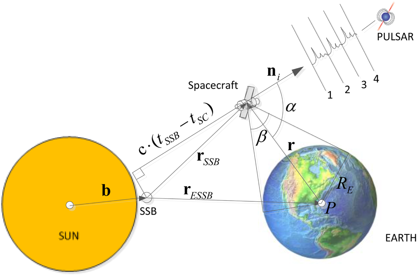
For simplicity, we call the direction vector-based X-ray pulsar navigation X-ray Pulsar Geometry Navigation (XPGN). The principle of XPGN is shown in Figure 1. To determine the radiation direction of the pulsar signal, a collimator is placed on the front of the detector to limit its field of view. The photons captured by the detector only come from a small section of the sky defined by the collimator. This characteristic will be used to obtain the incident direction of the pulsar signal to high precision, which can be expressed as the normalised pulsar position vector ni. At the same time, the detector can also record the TOAs of photons. Our aim is to utilise both the TOAs and the vector ni to estimate the position and velocity of the spacecraft. To simplify the issue, it is assumed that the Earth obstruction problem does not arise. The proposed method can be summarised as the following stages: (1) signal detection using X-ray detectors, (2) direction vector estimation and recording the timing data, (3) position estimation using ADDF. The proposed system structure is summarised in Figure 2. All the parts will be discussed in the following sections.

Figure 1. Principle of X-ray Pulsar Geometric Navigation (XPGN).
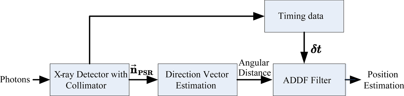
Figure 2. Structure of the proposed navigation system.
3. PULSAR POSITION VECTOR DETERMINATION
3.1. Model of the collimator
Collimators are a set of elongated well-type pipings made of special materials, which can limit the field of view to reduce X-ray background noise (Takahashi et al., Reference Takahashi, Abe, Endo, Endo, Ezoe, Fukazawa, Hamaya, Hirakuri, Hong, Horii, Inoue, Isobe, Itoh, Iyomoto, Kamae, Kasama, Kataoka, Kato, Kawaharada, Kawano, Kawashima, Kawasoe, Kishishita, Kitaguchi, Kobayashi, Kokubun, Jun'ichi, Kouda, Kubota, Kuroda, Madejski, Makishima, Masukawa, Matsumoto, Mitani, Miyawaki, Mizuno, Mori, Mori, Murashima, Murakami, Nakazawa, Niko, Nomachi, Okada, Ohno, Oonuki, Ota, Ozawa, Sato, Shinoda, Sugiho, Suzuki, Taguchi, Takahashi, Takahashi, Shin'ichiro, Ken-Ichi, Tamura, Tanaka, Tanihata, Tashiro, Terada, Shin'ya, Uchiyama, Watanabe, Yamaoka, Yanagida and Yonetoku2007). A perfectly aligned collimator can achieve the maximum transparency when it is parallel to the direction of the incoming ray. In other words, if the collimator points exactly at the X-ray source, the maximum number of photons can be captured in a unit time interval. Collimators can be simplified as tubes with walls dense and thick enough to block the incident path of the photons.
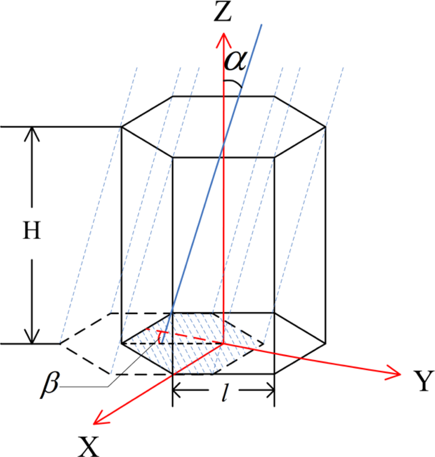
The cross section of the tube is a hexagon (Takahashi et al., Reference Takahashi, Abe, Endo, Endo, Ezoe, Fukazawa, Hamaya, Hirakuri, Hong, Horii, Inoue, Isobe, Itoh, Iyomoto, Kamae, Kasama, Kataoka, Kato, Kawaharada, Kawano, Kawashima, Kawasoe, Kishishita, Kitaguchi, Kobayashi, Kokubun, Jun'ichi, Kouda, Kubota, Kuroda, Madejski, Makishima, Masukawa, Matsumoto, Mitani, Miyawaki, Mizuno, Mori, Mori, Murashima, Murakami, Nakazawa, Niko, Nomachi, Okada, Ohno, Oonuki, Ota, Ozawa, Sato, Shinoda, Sugiho, Suzuki, Taguchi, Takahashi, Takahashi, Shin'ichiro, Ken-Ichi, Tamura, Tanaka, Tanihata, Tashiro, Terada, Shin'ya, Uchiyama, Watanabe, Yamaoka, Yanagida and Yonetoku2007) (see Figure 3) whose side-length is l and the height of the collimator is H. We set the angle between the line of collimator sight and the pulsar radiation direction to be θ. Before the photon reaches the detector, it should pass through the collimator's piping. The collimator walls shadow the detector and reduce the effective area which is illustrated by the shaded (back slant) region in Figure 3. As the hexagon is symmetrical with respect to its diagonal, the solution of the effective area can be divided into six equal cases. In other words, if S(α, β) indicates the effective area, then S(α, β) = S(α, β + mπ/3), where m = 0, 1, … 5, and each m corresponds to one case. More details are shown in Figure 4. If the centre point of the top cross projected at the P of the bottom and the region spanned by the diagonals OC and OD is OCD, one of the six cases can be defined using the P in the OCD.

Figure 3. Sketch of a hexagonal collimator.
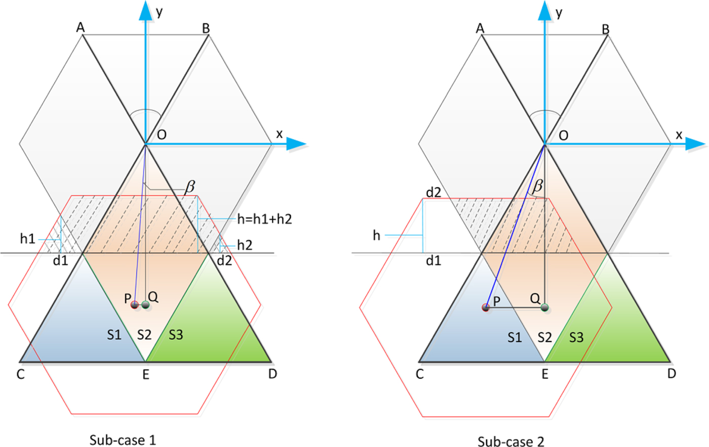
Figure 4. Effective area defined by the hexagon collimator.
To model the area, each case can be divided into two sub-cases. Sub-case 1 means that the P belongs to the region S2. Mathematically, sub-case 1 is given by:
 $$sc1=\left\{\matrix{\sin\lpar \vert\vert \beta\vert+\pi/6\rpar^{\ast}L_{OP}\lt \displaystyle{{\sqrt{3}}\over{2}}l \cr \vert\beta\vert\leq\displaystyle{{\pi}\over{6}}\hfill}\right. $$
where L OP is the length of the side OP, which is defined by L OP = Htanθ. Likewise, sub-case 1 means the P belongs to the region S1 and S3, as the S1 and S3 are symmetrical with respect to the y axis. So, sub-case 2 can be mathematically expressed as:
 $$sc2=\left\{\matrix{\sin\lpar \vert\beta\vert+\pi/6\rpar^{\ast}L_{OP}\geq \displaystyle{{\sqrt{3}}\over{2}}l \cr \vert\beta\vert\leq\displaystyle{{\pi}\over{6}}\hfill}\right. $$
In sub-case 1 the effective area can be expressed as the subtraction of the back-slant region and the slant region. The back-slant region is a trapezoid, whose height is given by:
 $$h=L_{OE}-L_{OQ}=\sqrt{3}l-H\tan\lpar \alpha\rpar \cos\lpar \beta\rpar $$
and the length of the top side is equal to l, that is:
 $$L_{top}=l $$
The length of the bottom side is calculated by:
 $$L_{bottom}=2h\tan\left(\displaystyle{{\pi}\over{6}}\right)+l $$
The slant region has two triangle parts whose height are h1 and h2 as shown in Figure 4. It is easy to find that h = h1 + h2. The bottom sides of the two triangles are d1 and d2, and it is easy to find:
 $$d1+d2=L_{bottom}-L_{op} $$
Hence, the effective area of sub-case 1 is given by:
 $$\eqalign{S & =\lpar L_{bottom}+L_{top}\rpar \displaystyle{{h}\over{2}}-\left(\displaystyle{{h1d1}\over{2}}+\displaystyle{{h2d2}\over{2}}\right)\cr & =hl+\displaystyle{{\sqrt{3}}\over{3}}h^{2}-\displaystyle{{\sqrt{3}}\over{4}}\lpar d1^{2}+d2^{2}\rpar } $$
For sub-case 2, the h, L top and L bottom can be calculated by using Equations (3), (4) and (5) as in sub-case 1, respectively. The d1 can be expressed as the sum of the L PQ = Htanαsinβ and the (L bottom − L top)/2, that is:
 $$d1=H\tan\alpha \sin\beta+h\tan\left(\displaystyle{{\pi}\over{6}}\right)$$
The d2 can be calculated using:
 $$d2=d1-2h\tan\left(\displaystyle{{\pi}\over{6}}\right)=H\tan\alpha\sin\beta-h\tan\left(\displaystyle{{\pi}\over{6}}\right)$$
Then, the effective area in sub-case 2 is given by:
 $$\eqalign{S & =\lpar L_{bottom}+L_{top}\rpar \displaystyle{{h}\over{2}}-\lpar d1+d2\rpar \displaystyle{{h}\over{2}} \cr & = h^{2}\tan\left(\displaystyle{{\pi}\over{6}}\right)+lh-hH\tan\alpha\sin\beta} $$
Substituting Equation (3) into Equation (7) and Equation (10), the effective error can be expressed as:
 $$S\lpar \alpha\comma \; \beta\rpar = \left\{\matrix{hl+\displaystyle{{\sqrt{3}}\over{3}}h^{2}-\displaystyle{{\sqrt{3}}\over{4}}\lpar d1^{2}+d2^{2}\rpar \comma \; \quad \hbox{for}\, sc1 \hfill\cr h\left(2l-\displaystyle{{\sqrt{3}}\over{3}}H\tan\alpha\, \cos\beta-H\tan\alpha\, \sin\beta\right)\comma \; \quad \hbox{for}\, sc2\hfill}\right. $$
where  $h=\lpar \sqrt{3}l-H\tan\alpha\cos\beta\rpar $, sc1 and sc2 mean the condition of sub-case 1 and sub-case 2 of Equation (11), respectively.
For simplicity, let A e = S(α, β). Since the number of captured photons is proportional to the effective area A e, the photon arrival rate at the detector can be written as:
 $$Ph\lpar \theta\rpar =I_{in}\varepsilon A_{e} $$
where I in is the flux density in unit area and λ is the efficiency of the X-ray detector.
From Figure 3, A e is maximum when the direction of the source is perpendicular to the area of the collimator due to the lack of shadows. That is, when θ = 0, the detector can obtain the maximum count rate of photons, which can be summarised as that at the point θ = 0, the right derivative of Equation (11) exists, and Equation (11) is monotonically decreasing for  $0\leq\theta \lt \arctan\ \lpar 2r/h\rpar $. Consequently, S(α, β) approaches its maximum value when θ → 0.
θ = 0 means the central axis of the collimator is parallel to the pulsar position vector. Thus, the purpose of the searching method is to adjust the pointing direction of the collimator to minimise θ, or to maximise Equation (12). Therefore, the vector searching issue can be expressed as the following optimisation problem:
 $$\hat{\theta}= \mathop{\hbox{argmax}\ Ph\lpar \theta\rpar }\limits_{0\leq\theta \lt \arctan\lpar 2r/h\rpar }= \mathop{\hbox{argmax}\ I_{in}\varepsilon A_{e}}\limits_{0\leq\theta \lt \arctan\lpar 2r\comma h\rpar } $$
Since I in and ε are independent of A e, Equation (13) can be simplified as:
 $$\hat{\theta}=\mathop{\hbox{argmax}\ A_{e}}_{0\leq\theta \lt \arctan\lpar 2r/h\rpar } $$
 The existence of  $\hat{\theta}$ is logical.
3.2. Orbit dynamic model
The satellite state dynamics are selected to establish the state equation of the system within the J2000·0 Earth-Centred Inertial (ECI) coordinate system. Let r denote the position vector of the spacecraft. The state vector is composed of the position and velocity vectors, which can be written as  ${\bf X}=\lsqb {\bf r}^{{\rm T}}\comma \; \ {\bf v}^{{\rm T}}\rsqb ^{{\rm T}}=\lsqb x\comma \; y\comma \; {\bi {z}}\comma \; {\bi {v}}_{X}\comma \; {\bi {v}}_{y}\comma \; {\bi {v}}_{Z}\rsqb ^{{\rm T}}$. The satellite state dynamics can be expressed as:
 $$\dot{{\bf X}}\lpar t\rpar =f\lpar {\bf X}\lpar t\rpar \comma \; t\rpar +{\bf w}\lpar t\rpar \comma \; $$
where  $\dot{{\bf X}}\lpar t\rpar =\lsqb \dot{{\bf r}}^{{\rm T}}\comma \; \dot{{\bf v}}^{{\rm T}}\rsqb ^{{\rm T}}=\lsqb {\bf v}^{{\rm T}}\comma \; {\bf a}^{{\rm T}}\rsqb ^{{\rm T}}$ is the satellite state dynamic equation, and w(t) is the process noise. By integrating Equation (15), we obtain the state transition equation:
 $${\bf X}\lpar t\rpar ={\bf X}\lpar t_{0}\rpar +\vint_{0}^{t}f\lpar {\bf X}\lpar \tau\rpar \comma \; \tau\rpar d\tau $$
 In  $\dot{{\bf X}}\lpar \hbox{t}\rpar =\lsqb {\bf v}^{{\rm T}}\comma \; {\bf a}^{{\rm T}}\rsqb ^{{\rm T}}$, the main parts of acceleration a include the two-body acceleration effect, the non-spherical Earth gravitational potential effect, and the third body gravitational effect from the sun and the moon. In this paper, the non-spherical gravitational perturbation is modelled as a two-order aspherical potential function. The details of the orbit dynamic model can be found in Liu et al. (Reference Liu, Fang, Yang, Kang and Wu2015) and Wei et al. (Reference Wei, Jin, Zhang, Liu, Li and Yan2013).
3.3. Definition of coordinate frames
From the model of the collimator, we find that the detector should be able to change its orientation continuously. A gimbal which is usually used in aerospace engineering is suitable for this purpose. Here, it is assumed that the detector is fixed on a two-degree gimbal.
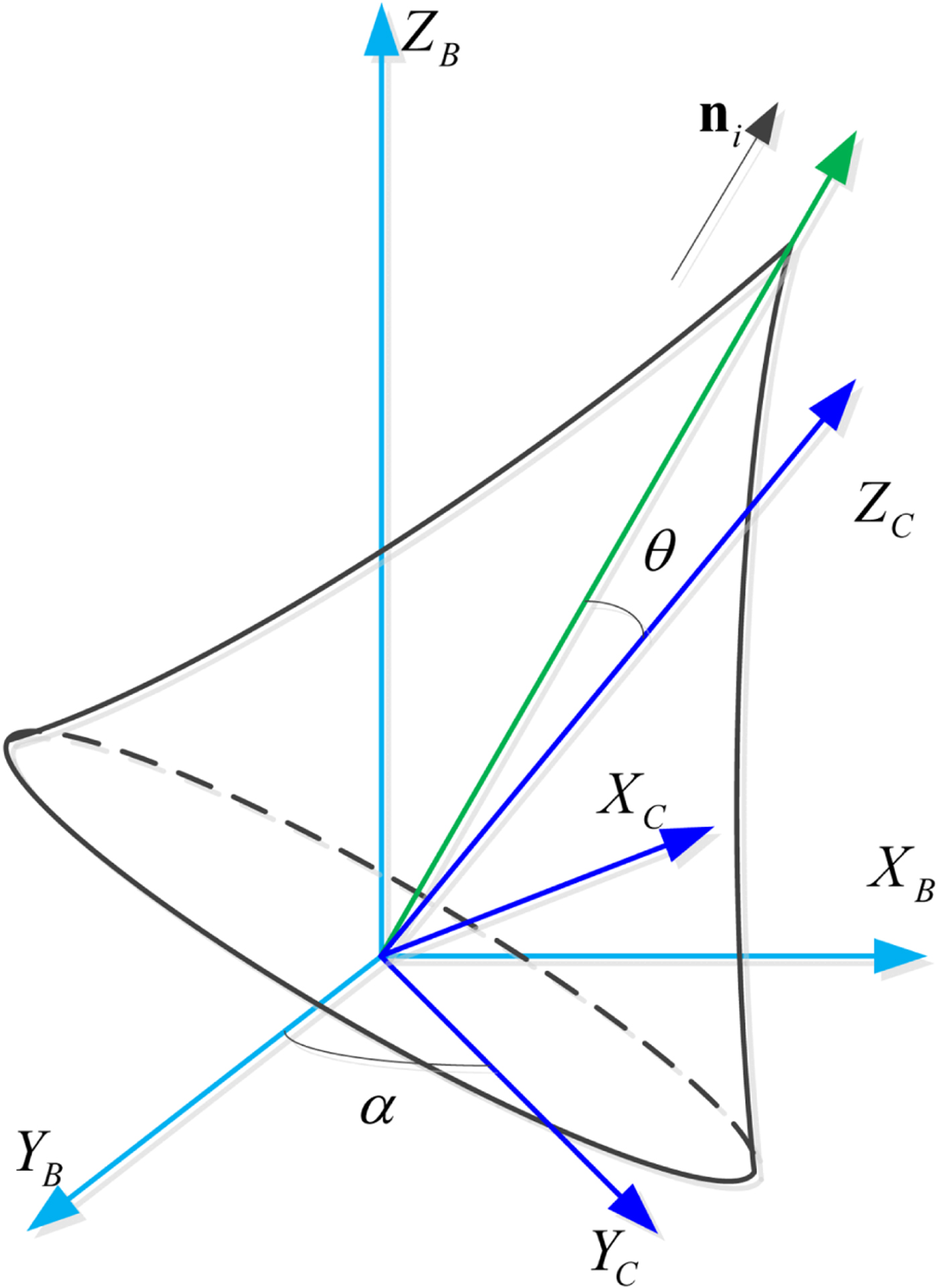
To fully describe the searching procedure, the coordinate frames should be defined. Therefore, two frames are defined as follows and shown in Figure 5.
(1) The body frame (B-frame) has its origin at the centre of mass of the vehicle. Its X-axis points along the longitudinal axis of the vehicle. The Z-axis is perpendicular to the longitudinal plane and the Y-axis completes the right handed system. In Figure 5, the body frame is expressed by the axes (X B, Y B, Z B).
(2) The collimator frame (C-frame) is expressed by (X c, Y c, Z c). Y c is parallel to the gimbal's horizontal axis. Z c points along the central axis of the collimator and X c is perpendicular to Y c and Z c Obviously, the angle between Z c and the pulsar direction ni is the error angle of θ in Figure 4. For simplicity, the origin of the C-frame is the same as for the B-frame.

Figure 5. Geometry relationships of the search procedure.
3.4. Vector searching strategy
The purpose of the searching strategy is to reduce θ via changing the pointing direction of the collimator, Z c. In Figure 5, the circular cone describes the relationship between the photon intensity passing through the collimator and the error angle θ. It should be noted that the horizontal axis of the gimbal can only spin in one plane, which means that, in Figure 4, X c can only rotate a in the plane spanned by (X c, Y c) around Z B. The pointing direction of the collimator, Z c, spins around X c. As X c and Z c are orthogonal, the rotation of each axis will change θ in a linearly independent direction. This makes the searching procedure quite suitable for the Powell method (Powell, Reference Powell1964). Two conditions should hold: (a) the recorded flux intensity can be formulated as a function of θ; and (b) this function is convex. Equation (12) shows that the two conditions can be satisfied. Based on the modified Powell method, the searching strategy can be summarised as follows:
(1) Given a priori knowledge of the attitude information, the vehicle estimates the coarse position of the target pulsar in the B-frame from the reference pulsar catalogue. The gimbaled X-ray detector attempts to adjust the central axis to the pulsar direction to acquire pulsar signals. The on board computational system detects the target signal in real time using the Fast Fourier Transform (FFT) proposed in our previous works (Zhang and Xu, Reference Zhang and Xu2011). When successful, go to Step (2).
(2) In the B-frame, Xc can be expressed by the vector (cosα, sinα, 0) T. If X c rotates around Z B by Δ a, the new vector becomes (cos(α + Δα), sin(α + Δα), 0) T. Here, we use quaternions to express the rotation of Z c about X c (Bar-Itzhack and Oshman, Reference Bar-Itzhack and Oshman1985). Let β be the rotational angle and X c the rotational axis. The quaternion is:
(17) $$\hat{q}=q_{0}+q=\cos\lpar \beta/2\rpar +\sin\lpar \beta/2\rpar \lpar \cos\alpha+\Delta\alpha\comma \; \sin\alpha +\Delta\alpha\comma \; 0\rpar ^{T} $$
Let
$\vec{v}_{c}$ be the unit vector along the Z c axis. The rotation of Z c about X c by angle β can be written as $L_{v}=\hat{q}\vec{v}_{c}\hat{q}^{\ast}$. Then, the searching strategy procedure is given as follows:
(a) Set the initial point x(0) = (α 0, β 0) and two linear independent directions α 1, β 1. The permissible error is ε ≥ 0 and k = 1.
(b) Set x(k,0) = x(k−1). From x(k,0), search along the direction αk using a linear search method:
(18)$$\min_{\lambda}\ \hbox{ph}\lpar \theta\rpar =f\lpar x^{\lpar k\comma 0\rpar }+\lambda\alpha^{k}\rpar . $$The result is x(k,1). Similarly, we can obtain the point xk by searching along the direction β k and x(k,1) is the initial point.
(c) If ‖ ph (θ) − phmax‖ ≤ ε, go to Step (3), where phmax is the average maximum flux intensity of the source recorded by the detector. Otherwise, let x0 = xk, then return to (a).
(3) The detector keeps observing the target pulsar and the average flux intensity of the computing system. If | ph (θ) − phmax‖ > ε, go to Step(2)-(a), and adjust the pointing direction again.


4. MODELS OF AUTONOMOUS ORBIT DETERMINATION
4.1. Orbit determination by using pulsar vector observation
If the collimator points to the pulsar, a geometrical navigation method can be derived. As shown in Figure 1, the angle between the pulsar direction vector and the geocentric direction vector can be formulated by using a satellite orbit position. The unit vector of Earth's centre with respect to the satellite can be obtained by the infrared or ultraviolet horizon sensor. In Figure 1, r is the direction vector pointing from the Earth's centre to the satellite. α is the angle between r and the pulsar's line of sight vector ni. Then, the observation equation of XPGN can be written as:
 $$\alpha =h\lpar {\bf r}\comma \; t\rpar =\hbox{arccos} \left(- \displaystyle{{{\bf r}\cdot {\bf n}_{i}}\over{\vert{\bf r}\vert}}\right)+n_{\alpha} $$
where ni can be obtained by the searching method proposed in Section 3.3. n α is the random error of α and is assumed to be Gaussian noise, and  ${\bf x}=\lsqb {\bf r}^{{\rm T}}\comma \; \dot{{\bf r}}^{{\rm T}}\rsqb ^{{\rm T}}$ is the satellite state in the ECI coordinate frame. Linearization of Equation (19) at the predicted state X* can be expressed as:
 $$\alpha =h\lpar {\bf r}^{\ast}\comma \; t\rpar + \displaystyle{{\partial h}\over{\partial {\bf r}}}\vert_{{\bf r}-{\bf r}^{\ast}}\lpar {\bf r}-{\bf r}^{\ast}\rpar +n_{\alpha} $$
Let δ r = r − r* denote the position error. δα = α − h(r*, t) expresses the observational residual. Equation (20) can be rewritten as:
 $$\delta\alpha={\bf G}^{T}\delta {\bf x} +n_{\alpha} $$
where  $\delta {\bf x} =\lsqb \delta {\bf r}^{{\rm T}}\comma \; \delta\dot{{\bf r}}^{{\rm T}}\rsqb ^{{\rm T}}$ and G are the observation matrices. Since:
 $$\eqalign{\displaystyle{{\partial h}\over{\partial {\bf r}}} & =\displaystyle{{1}\over{\sin\alpha}}\left(\displaystyle{{{\bf n}_{i}}\over{\vert{\bf r}\vert}}-\displaystyle{{\lpar {\bf r}\cdot {\bf n}_{i}\rpar {\bf r}}\over{\vert{\bf r}\vert^{3}}}\right)\cr &=\displaystyle{{1}\over{\vert{\bf r}\vert\sin\alpha}}\left({\bf n}_{i}+\displaystyle{{{\bf r}}\over{\vert{\bf r}\vert}}\cos\alpha\right)} $$
and:
 $$\displaystyle{{\partial h}\over{\partial\dot{{\bf r}}}}={\bf 0} $$
G can be written as:
 $${\bf G}=\left[\matrix{\displaystyle{{\partial h}\over{\partial {\bf r}}} \cr \displaystyle{{\partial h}\over{\partial\dot{{\bf r}}}}}\right]= \left[\matrix{\displaystyle{{1}\over{\vert{\bf r}\vert\sin\alpha}}\left({\bf n}_{i}\quad +\displaystyle{{{\bf r}}\over{\vert{\bf r}\vert}}\cos\alpha\right)\cr \qquad {\bf 0}}\right]$$
where  $\cos\alpha=\displaystyle{{\lpar -{\bf r}\rpar \cdot{\bf i}_{{\bf i}}}\over{\vert{\bf r}\vert}}$.
4.2. Orbit determination using timing data
Orbit determination by using timing data is the fundamental task in XPNAV. In this method, the captured photon sequences are utilised to obtain the pulse Time Of Arrival (TOA) (Sheikh, Reference Sheikh2005), while the corresponding TOA at the SSB can be predicted by the pulsar timing model. The offset between measured TOA and predicted TOA can be used to correct the position error.
The geometric relationship of the sun, the X-ray pulsar and the navigation satellite in the SSB coordinate system is shown in Figure 1. Here, c is the speed of light and b is the position of the SSB relative to the barycentre of the Sun. rSSB denotes the position vector of the spacecraft with respect to the SSB and rESSB denotes the position of the Earth's centre with respect to the SSB.
To get the navigation observation of the X-ray pulsar, the TOA measured at the spacecraft, t SC, must be transferred to the corresponding time at the SSB where the pulsar timing model is defined. Let D 0 denote the range between the pulsar and the SSB. Let the solar gravitational constant be μSun. The term of  $O\lpar 1/D_{0}^{2}\rpar $ is a small value and negligible, so the transition equation can be given by (Sheikh, Reference Sheikh2005):
 $$\eqalign{t_{SSB}^{i}-t_{sc}^{i} & =\hbox{H}\lpar {\bf r}_{SSB}\comma \; {\bf n}_{i}\comma \; D_{0}\comma \; {\bf b}\rpar \cr & = \displaystyle{{{\bf n}_{i}\cdot {\bf r}_{SSB}}\over{C}}+\displaystyle{{1}\over{2cD_{0}}}\lsqb \lpar {\bf n}_{i}\cdot {\bf r}_{SSB}\rpar ^{2}-r_{SSB}^{2}+2\lpar {\bf n}_{i}\cdot{\bf b}\rpar \lpar {\bf n}_{i}\cdot{\bf r}_{SSB}\rpar \cr & \quad -2\lpar {\bf b}\cdot {\bf r}_{SSB}\rpar +2\lpar {\bf n}_{i}\cdot{\bf V}\Delta t_{N}\rpar \lpar {\bf n}_{i}\cdot{\bf r}_{SSB}\rpar \rsqb \cr & \quad +\displaystyle{{2\mu_{Sun}}\over{c^{3}}}\ln\left\vert\displaystyle{{{\bf n}_{i}\cdot {\bf r}_{SSB}+r_{SSB}}\over{{\bf n}_{i}\cdot {\bf b}+b}}+1\right\vert} $$
where i means the i-th pulsar, V is the proper motion of pulsars.  $\triangle t_{N}=t_{N}-t_{0}$ is the interval between the first pulse and the N-th pulse. As V is very small and D 0 ≫ VΔt, VΔt can be neglected. Let the measurement be expressed by
  $Z=c\lpar t_{SSB}^{i}-t_{SC}^{i}\rpar $, then the observation equation is written as:
 $$Z=h\lpar {\bf X}\comma \; t\rpar +v\lpar t\rpar $$
where:
 $$\eqalign{h\lpar {\bf X}\comma \; t\rpar & ={\bf n}_{i}\cdot {\bf r}_{SSB}+\displaystyle{{1}\over{2D_{0}}}\lsqb \lpar {\bf n}_{i}\cdot {\bf r}_{SSB}\rpar ^{2}-r_{SSB}^{2}+2\lpar {\bf n}_{i}\cdot {\bf b}\rpar \lpar {\bf n}_{i}\cdot{\bf r}_{SSB}\rpar -2\lpar {\bf b}\cdot {\bf r}_{SSB}\rpar \rsqb \cr & \quad + \displaystyle{{2\mu_{Sun}}\over{c^{2}}}\ln\left\vert\displaystyle{{{\bf n}_{i}\cdot {\bf r}_{SSB}+r_{SSB}}\over{{\bf n}_{i}\cdot {\bf b}+b}}+1\right\vert} $$
and v (t) is the noise. Supposing the predicted position vector of the satellite is  $\tilde{{\bf r}}_{SSB}$, the predicted TOA becomes:
 $$\tilde{t}_{sc}^{i}=t_{SSB}^{i}-{\bf H}\lpar \tilde{{\bf r}}_{SSB}\comma \; {\bf n}_{i}\comma \; D_{0}\comma \; {\bf b}\rpar $$
 Let the position error be  $\delta {\bf r}_{SSB}={\bf r}_{SSB}-\tilde{{\bf r}}_{SSB}$. Then the error of the predicted and measured pulse TOA can be defined as
  $\delta t_{SC}^{i}=t_{SC}^{i}-\tilde{t}_{SC}^{i}$. Substituting Equation (28) into Equation (25), and ignoring the high order items, the expression of TOA error at the spacecraft can be derived:
 $$\eqalign{\delta t_{sc}^{i} & =\hbox{H}\lpar \delta {\bf r}_{SSB}\comma \; {\bf n}_{i}\comma \; D_{0}\comma \; {\bf b}\rpar \cr &=-\displaystyle{{{\bf n}_{i}\cdot \delta{\bf r}_{SSB}}\over{c}}-\displaystyle{{1}\over{cD_{0}}}\lsqb \lpar {\bf n}_{i}\cdot\tilde{{\bf r}}_{SSB}\rpar \lpar {\bf n}_{i}\cdot\delta{\bf r}_{SSB}\rpar -\tilde{{\bf r}}_{SSB}\delta {\bf r}_{SSB} \cr & \quad +\lpar {\bf n}_{i}\cdot {\bf b}\rpar \lpar {\bf n}_{i}\cdot\delta{\bf r}_{SSB}\rpar -\lpar {\bf b}\cdot\delta{\bf r}_{SSB}\rpar \rsqb \cr & \quad -\displaystyle{{2\mu_{Sun}}\over{c^{3}}}\left[\displaystyle{{{\bf n}_{i}\cdot\delta{\bf r}_{SSB}+\tilde{{\bf r}}\cdot\delta{\bf r}_{SSB}/\tilde{r}_{SSB}}\over{{\bf n}_{i}\cdot\tilde{{\bf r}}_{SSB}+\tilde{r}_{SSB}+{\bf n}_{i}\cdot {\bf b}+b}}\right]} $$
 Let  $\delta {\bf x}_{SSB}=\lsqb \delta {\bf r}_{SSB}^{{\rm T}}\comma \; \delta\dot{{\bf r}}_{SSB}^{{\rm T}}\rsqb ^{{\rm T}}$ denote the state vector and the observation model for X-ray pulsars can be rewritten as:
 $$\delta {\bf y}={\bf H}_{i}^{T}\delta {\bf x}_{SSB}=\left[\matrix{ -\displaystyle{{{\bf n}_{i}}\over{c}}-\displaystyle{{1}\over{cD_{0}}}\lsqb \lpar {\bf n}_{i} \cdot \tilde{{\bf r}}_{SSB}\rpar {\bf n}_{i}-\tilde{{\bf r}}_{SSB} \cr +\, \lpar {\bf n}_{i}\cdot {\bf b}\rpar {\bf n}_{i}-{\bf b}\rsqb \cr -\displaystyle{{2\mu_{Sun}}\over{c^{3}}}\left[\displaystyle{{{\bf n}_{i}+\tilde{{\bf r}}_{SSB}/\tilde{r}_{SSB}}\over{{\bf n}_{i}\cdot\tilde{{\bf r}}_{SSB}+\tilde{r}_{SSB}+{\bf n}_{i}\cdot {\bf b}+b}}\right]\cr 0}\right]^{{\rm T}}\delta {\bf x}_{SSB}+w_{i}\lpar t\rpar $$
where  ${\bf H}^{T}_{i}=\hbox{H}^{T}\lpar \tilde{{\bf r}}_{SSB}\comma \; {\bf n}_{i}\comma \; D_{0}\comma \; {\bf b}\rpar $ and w i(t) is the Gaussian white noise. If several pulsars are observed at the same time, there is
  $\delta {\bf y}=\lsqb \delta t_{sc}^{1}\comma \; \, \delta t_{sc}^{2}\comma \; \, \cdots\, \comma \; \delta t_{sc}^{m}\rsqb ^{{\rm T}}$.
5. FILTERING ALGORITHM
Based on the observation of timing data and pulsar vectors, the ADDF is adopted as an iterative filter algorithm. The ADDF algorithm can be found in Dey et al. (Reference Dey, Sadhu and Ghoshal2015). This method integrated different observation equations linearly. Through Equations (21) and (30), we can get the combined observation vector  ${\bf Y}=\lsqb \delta\alpha_{1}\comma \; \delta\alpha_{2}\comma \; \cdots\comma \; \delta\alpha_{k}\comma \; \delta t_{sc}^{1}\comma \; \delta t_{sc}^{2}\comma \; \cdots\comma \; \delta t_{sc}^{m}\rsqb ^{{\rm T}}$, and:
 $$\eqalign{{\bf Y} & ={\bf H}^{{\rm T}}\delta {\bf X}+{\bf N\lpar t\rpar } \cr & = \lsqb {\bf G}_{1}^{{\rm T}}\comma \; {\bf G}_{2}^{{\rm T}}\comma \; \cdots\comma \; {\bf G}_{k}^{{\rm T}}\comma \; \ {\bf T}_{1}^{{\rm T}}\comma \; {\bf T}_{2}^{{\rm T}}\comma \; \cdots\comma \; {\bf T}_{m}^{{\rm T}}\rsqb ^{{\rm T}}\delta {\bf X}+{\bf N}\lpar t\rpar }$$
where  $\delta {\bf X}=\lsqb \delta {\bf r}_{E}^{{\rm T}}\comma \; \delta\dot{{\bf r}}_{E}^{{\rm T}}\rsqb ^{{\rm T}}$ and H denote the linearized measurement equations. N(t) is the Gaussian noise which is a zero-mean Gaussian function. N(t) can be expressed as:
 $${\bf N}\lpar t\rpar =\lsqb n_{\alpha_{1}}\comma \; n_{\alpha_{2}}\comma \; \cdots\comma \; n_{\alpha_{k}}\comma \; v_{1}\lpar t\rpar \comma \; v_{2}\lpar t\rpar \comma \; \cdots\comma \; v_{m}\lpar t\rpar \rsqb ^{{\rm T}}$$
The variance matrix of N(t) is:
 $${\bf R}\lpar t\rpar =diag\lpar \sigma_{\alpha_{1}}^{2}\comma \; \cdots\comma \; \sigma_{\alpha_{k}}^{2}\comma \; \sigma_{w_{1}}^{2}\comma \; \cdots\comma \; \sigma_{w_{m}}^{2}\rpar $$
where  $\sigma_{\alpha_{i}}^{2}$ is the variance of α, and
  $\sigma_{w_{i}}^{2}$ is the variance of the TOA of the i-th pulsar. so
  $\sigma_{w_{i}}$ can be defined as:
 $$\sigma_{w_{i}}=\displaystyle{{1}\over{2}}\displaystyle{{W_{i}}\over{SNR_{i}}} $$
where W i is the pulse width. SNR i is Signal-to-Noise Ratio of the i-th pulsar which is defined as:
 $$SNR_{i}=\displaystyle{{F_{X}Ap_{f}\triangle t_{obs}}\over{\sqrt{\lsqb B_{X}+F_{X}\lpar 1-p_{f}\rpar \rsqb \lpar A\triangle t_{obs}d_{i}\rpar +F_{X}Ap_{f}\triangle t_{obs}}}}\comma \; $$
where F X is the observed X-ray photon flux, B X is the X-ray background radiation flux, A is the area of the X-ray detector, p f is the pulsed fraction,  $\triangle t_{obs}$ denotes the observation time and d i is the duty cycle of a pulsar, which can be written as:
 $$d_{i}=\displaystyle{{W_{i}}\over{P_{i}}} $$
where P i is the pulse period.
Based on the observation Equations (21) and (30), we can formulate an optimal filter with the information from the pulsar direction vector and the TOA measurement.
Here, an ADDF is used to complete information fusion. It has the advantage of DDF and UKF with a second order Taylor's series approximation. Through adjusting the noise covariance matrix automatically, ADDF can also estimate process noise covariance. The performance of ADDF is outstanding in a situation where a priori knowledge of actual process noise covariance is absent. The structure is shown in Figure 6. The details of ADDF are presented in Dey et al. (Reference Dey, Sadhu and Ghoshal2015), and a numerical simulation is presented in Section 6.
Figure 6. Structure of ADDF.
As shown in Figure 6, the ADDF filter is used to obtain the local optimal state estimation Xi(k)(i = 1, 2) and the estimation error covariance matrix Pi(i = 1, 2). Then the global optimal state estimation ( $\hat{{\bf X}}_{g}$, Pg) is obtained.
6. NUMERICAL EXPERIMENTS
6.1. Searching strategy
6.1.1. Initial conditions
To verify the feasibility of the searching strategy, numerical simulation based on the proposed searching method is completed. A Global Positioning System (GPS) orbit (GPS BIIA-10) is chosen for the simulation. The parameters of the satellite orbit can be expressed as follows: the semi-major axis of the orbit is 4,164·3 km; the eccentricity of the orbit is 0·0116; the right ascension of the ascending node is 224·67°, the inclination is 54·39° and the argument of the perigee is 338·24°. Three pulsars are selected as the observation targets to complete the simulation and the parameters of the pulsars are listed in Table 1. For simplicity, we also assume that the area of the X-ray detector is 10,000 cm2 and that the background noise is 4·45e-l ph/cm2/s. These two parameters have been used in Sheikh and Pines' study (Reference Sheikh and Pines2006).
Table 1. Parameters of the pulsars used in the simulation

6.1.2. Searching with attitude error
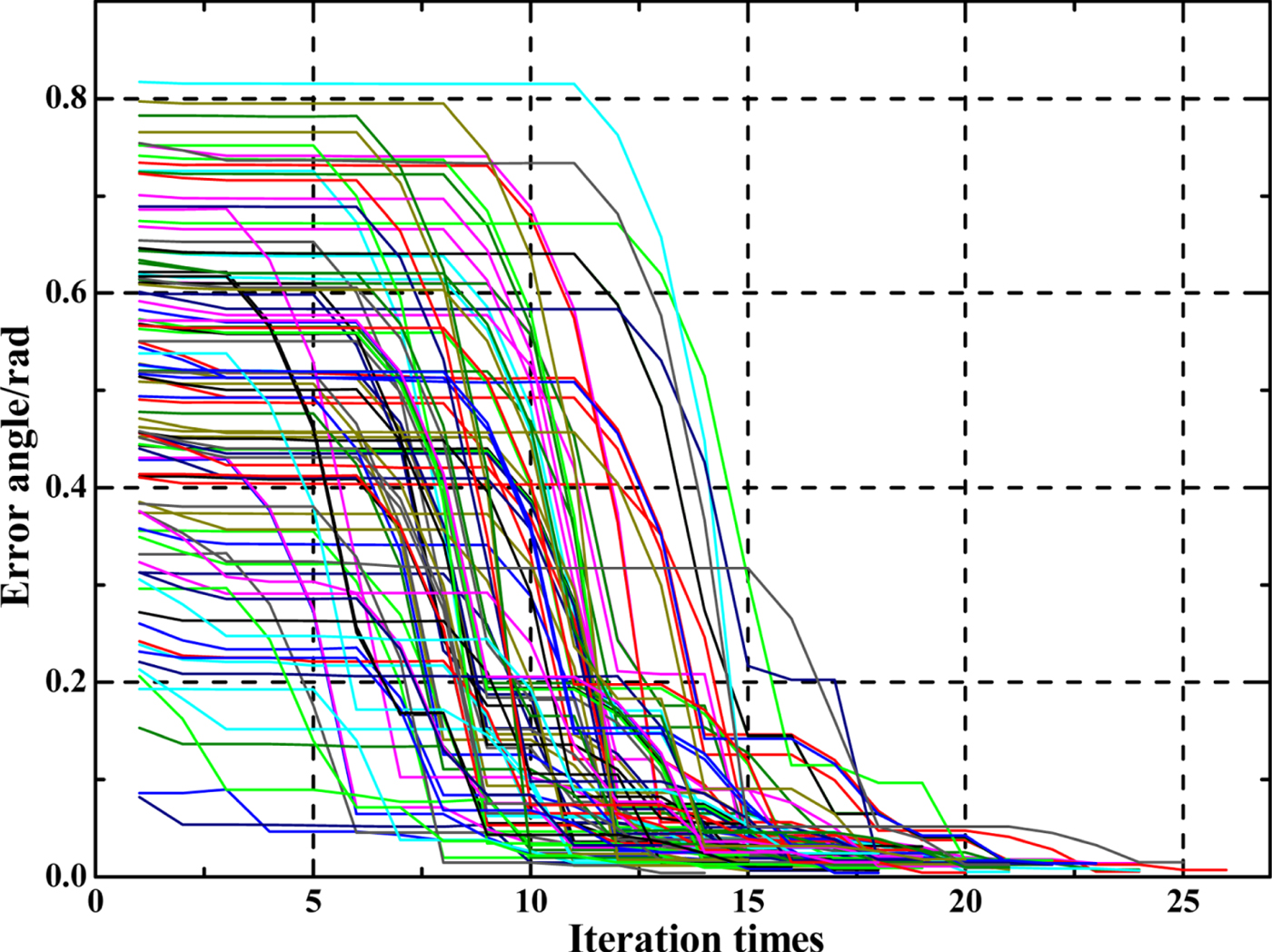
Figure 7 shows the simulation result of the searching strategy by using B0531 + 21 as the observation target.

Figure 7. Searching strategy simulation results.
As shown in Figure 5, the initial directions of X c and Z c will influence the searching procedure. One hundred Monte Carlo experiments have been done for the simulation. The selection strategy of the initial directions can be described as follows: (1) Assume the original attitude information is known and the pulsar is in the field view of the collimator, and the initial error angle θ, which is the angle between Z c and the pulsar direction ni, obeys a uniform distribution over [00·8] rad; (2) once the direction of Z c is set, X c is vertical to the plane spanned by Z c and Z B. In Figure 7, the vertical axis is the error angle θ and the horizontal axis is the iteration times. Each line in the figure represents one searching procedure with a different initial direction of X c and Z c. From the figure we can clearly see that the error angle between ni and Z c converges to zero for all lines, which means that the searching method is an asymptotic convergence. In most cases, it must run more than six iteration times to enter the fast convergence stage. This is because the flux intensity is very small at the beginning of the searching process. However, with different initial pointing directions of X c and Z c, the number of required iteration steps for convergence varies from 15 to 20 in most cases.
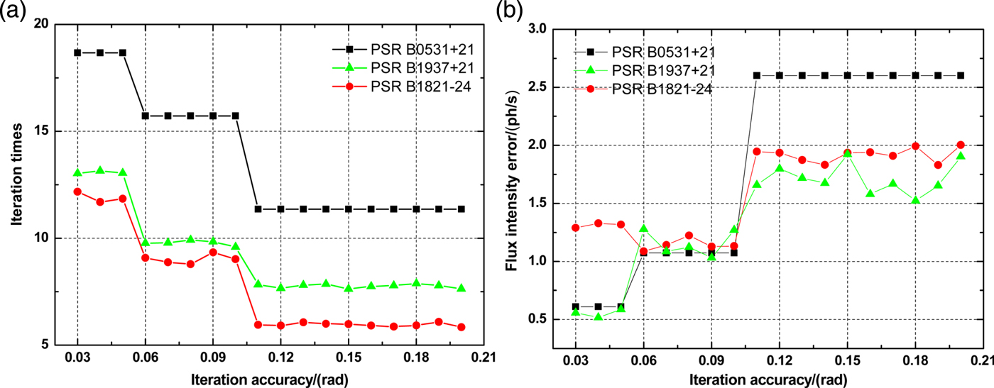
6.1.3. Permissible error and convergence accuracy
Figure 8 shows the influence of the permissible error, ε, on the iteration times and searching accuracy. The permissible error is used to terminate the linear searching process when the searching result reaches a certain accuracy. According to the precision limitation of the gimbal, the minimum value of ε is set to be 2·25e-2 rad. First, with a fixed permissible error and the random initial directions, 100 searching attempts are conducted. The number of iterations for convergence and the searching errors between the theoretical flux intensity and the searching results are averaged. Then we choose 20 different permissible errors to repeat the former process. Figure 8(a) shows the influence of permissible error ε on the average iteration times. Figure 8(b) shows the variation of the searching error with the permissible error. In Figure 8(a), when ε increases, the required iteration times for the method to converge decrease. This means that with a larger permissible error, it will take less time for the method to obtain satisfactory searching results. Increasing ε will result in larger searching errors as shown in Figure 8(b). We can also see from the figure that when the permissible error becomes too large, the curve becomes flat. The reason for this is that when the permissible error is too large, the linear searching process will terminate too early to reach the target. This is also the reason why when the permissible error becomes large, the flux intensity error increases as shown in Figure 8(b).

Figure 8. Influence of permissible error.
6.2. Filtering algorithms
6.2.1. Initial conditions
In this section, we choose the same GPS orbit as in Section 6.1, and the parameters of the pulsars are listed in Table 1. The initial state errors of object satellite is δX(0) = [2km 2km 2km 10m/s 10m/s 10m/s]T. The position error and velocity error are defined as:
 $$deltX = \sqrt{\vert\hat{{\bf r}}-{\bf r}\vert^{2}}$$
 $$deltV = \sqrt{\vert\hat{\dot{{\bf r}}}-\dot{{\bf r}}\vert^{2}} $$
where r = (x, y, z) is the position vector and  $\dot{{\bf r}}=\lpar v_{x}\comma \; v_{y}\comma \; v_{Z}\rpar $ is the velocity of the vehicle.
  $\hat{{\bf r}}$ and
  $\hat{\dot{{\bf r}}}$ are the estimation of r and
  $\dot{{\bf r}}$, respectively. The initial covariance matrix of the process noise w(t) is Q = diag((20m)2 (20m)2 (20m)2 (1m/s)2 (1m/s)2 (1m/s)2).
The vector observation of the pulsar is conducted by the searching method proposed in Section 3.3. Based on the simulation process in Section 6.1, the permissible error ε of the searching procedure is set to be 2·25e-5 rad. We made 100 Monte Carlo experiments of the vector searching strategy to calculate the statistical variance of the error angle, then transformed it into position error according to the inverse function of Equation (26). Simultaneously, taking the error of the Earth centre point into account, the variance of the vector is set to be Rv = [(2·25e - 5rad)2, (2·25e - 5rad)2, (2·25 - 5rad)2]T. Similarly, according to Equation (34), the covariance matrix of measurement noise of three pulsars' timing observations can be expressed as Rp = [(0 · 11km) 2, (0 · 32km) 2, (0 · 34km) 2] T.
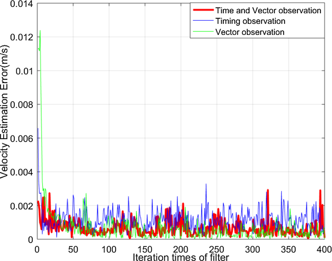
6.2.2. Filtering algorithms simulation
To demonstrate the performance of the proposed method, three cases are designed. Case 1 uses the Vector observation. Case 2 uses the timing observation. Case 3 uses the timing data and the vector observation simultaneously as has been stated in Section 5. All three cases use an ADDF as the Filter algorithm. The pulsars used in the simulation are listed in Table 1. The results are shown in Figures 9 and 10, respectively. Figure 9 illustrates the position estimation error versus iteration times. It can be seen that if only the vector observation is used, the result has the maximum estimation error and the slowest convergence rate. This is because the pulsar orientation vector estimation is not high enough. In comparison, the filter result using the timing data is better under the simulation condition. It is expected that the pulsar orientation vector can improve the navigation performance by using the integrated ADDF method introduced in Section 5. The result is also illustrated in Figure 9. It is obvious that when the timing data and the vector observation are both used, the ADDF has the minimum error, and the filter curve is the smoothest. The statistical data is shown in Table 2. The variance of position error can decrease from 0·3588 km2 to 0·0485 km2 by adding the orientation vector measurement. To make it clearer, the accumulative errors of the three methods are presented in Figure 11. The ordinate and abscissa of Figure 11 are accumulative position errors and iteration times, respectively. It is easy to see that the integrated ADDF using the timing data and the orientation vector has the minimum accumulative errors. The velocities of three cases are also compared, and the results are shown in Figure 10. It should be pointed out that the velocity variances of the integrated method are not distinguishable from the curves in Figure 10. The data in Table 2 explains the issue. It illustrates that if only the timing data are used, the magnitude of the adjustment of the velocity is maximum. In contrast, the variance of the velocity is minimum when the orientation vector is adopted.
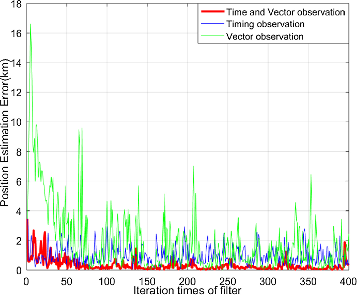
Figure 9. Position estimation errors.

Figure 10. Velocity estimation errors.
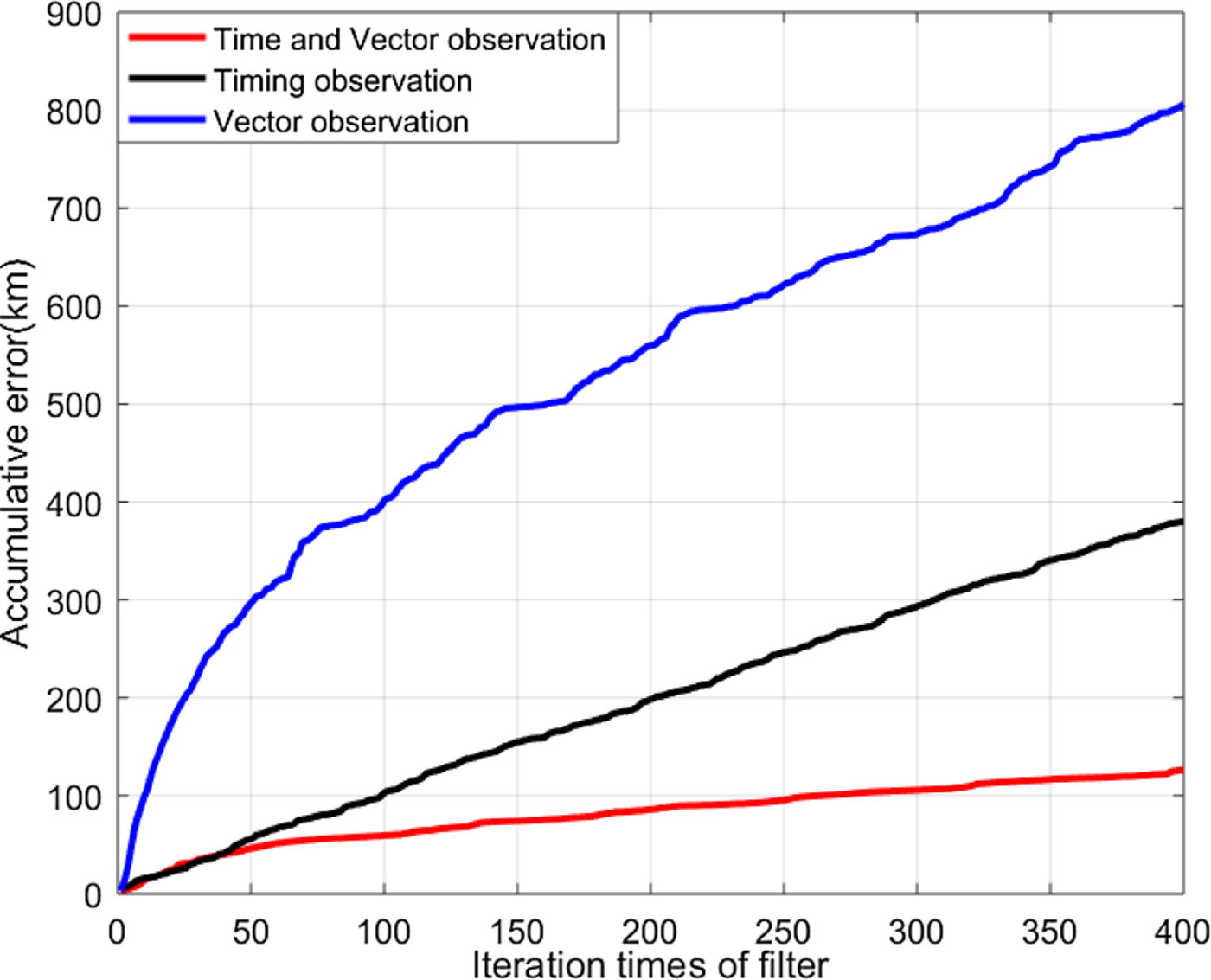
Figure 11. Accumulative errors of different methods.
Table 2. Average estimation errors of different algorithms

In summary, the accuracy of position by using the time and vector observations is improved by 75% over the traditional XPNAV with the ADDF filter. Compared with the vector observation alone, the position accuracy with the improved method can reach up to 80% by employing an ADDF. Looking at the three cases, one can see that the performance of the ADDF is improved with the increasingly effective observation information, which illustrates the effectiveness of the improved method.
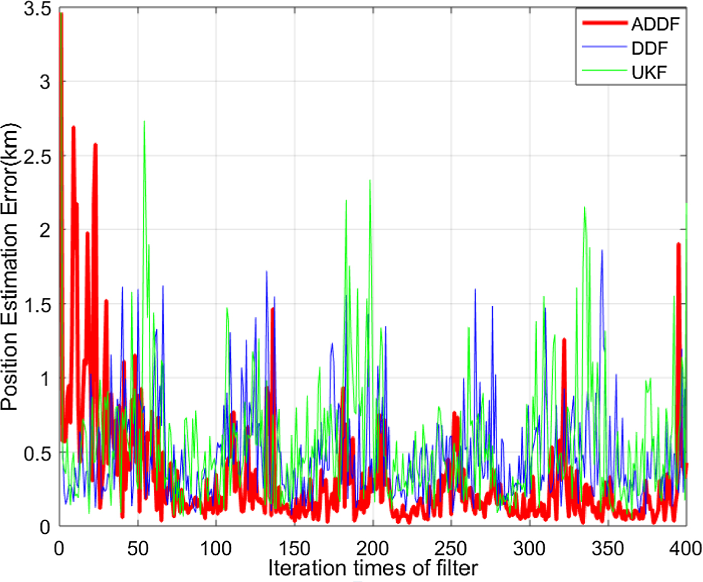
To illustrate the performance of the ADDF, a comparison of differences between ADDF, Divided Difference Kalman Filter (DDF) and Unscented Kalman Filter (UKF) are shown in Figures 12–14 by using the timing data and position vectors together. Statistical comparison results are presented in Table 3.

Figure 12. Position estimation errors.
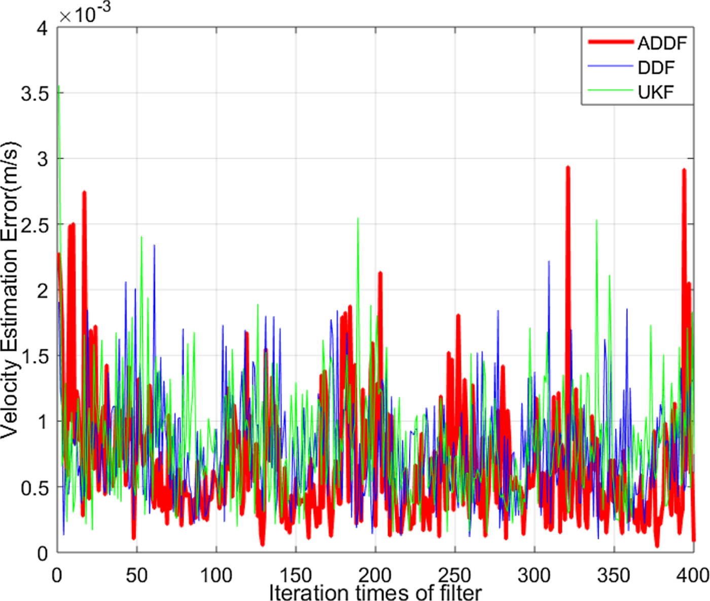
Figure 13. Velocity estimation errors of different filters of different filters.
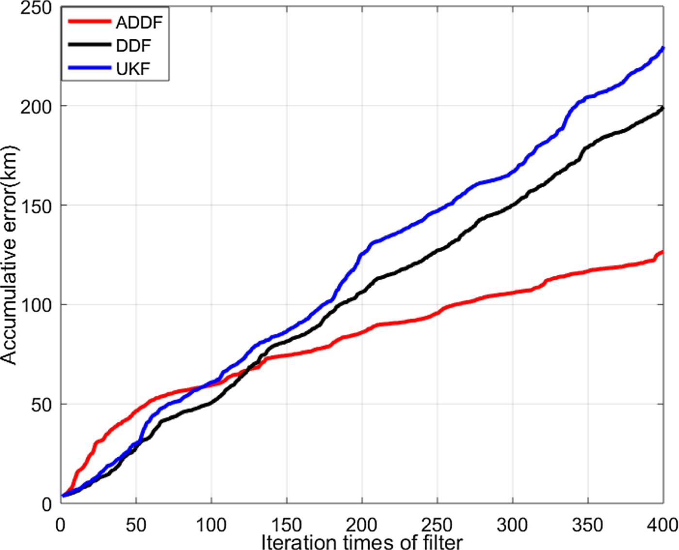
Figure 14. Accumulative errors of different filters.
Table 3. Estimation error of different filters
In Figures 12–14, the abscissa corresponds to iteration times of filtering and ordinate denotes the position or velocity estimation error. In Figure 14, the ordinate denotes the accumulative error. From the simulation results, it can be seen that the performance of DDF is slightly better than the UKF. Of these three filters, the ADDF filter has the best navigation precision by adjusting the covariance matrix of process noise. Table 3 gives the statistical results of different filters. The data shown in Table 3 indicates that the precision of position by using ADDF is improved by 60% and 54%, respectively, compared with UKF and DDF, while the velocity improvement reaches up to 30% and 26%. The character of the ADDF filter will be extremely valuable in a situation where the process noise is hard to calculate in XPNAV.
6.2.3. Effect of installation error
The installation errors of the pointing mechanism will affect the pulsar direction vector measurement. These errors can be divided into two types. The first is the system error, which can be treated as a constant error and can be deducted by refining the system model. The second is random errors coming from the mechanical errors, which cannot be simply removed from the result and must use an estimation method such as a Kalman filter. It is obvious that system error will lead to filter convergence to the wrong mean value. The random errors can be generally treated as Gaussian noise, which will increase the variance of the filter results. To explain the effect of the random errors, we use the cumulative error of the DDF to show the results.
In the simulation, the DDF filter is adopted to estimate the performance. The installation error will increase the permissible ε. We increase the error from 2·25e-6 rad to 2·25e-4 rad. From Figure 15 and Table 4, it can be seen that, with the increase of ε, the estimation error and the cumulative error of navigation of the satellite gradually increases. The data is shown in Table 4. So the installation errors should be decreased as much as possible.
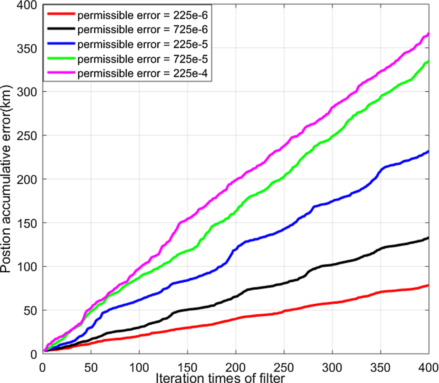
Figure 15. The cumulative error versus iteration times.
Table 4. The data of Figure 15

7. CONCLUSIONS
A novel method using pulsar position vectors to improve the performance of X-ray pulsar-based navigation has been presented. The main works of this paper can be summarised as the model and searching strategy of the position vector and the navigation model based on position vector and timing data. As for position vector observation, the field of view of the collimator was used to scan the target pulsar source, and the pulsar position vector was estimated by maximising the incident flux density recorded by the X-ray detector. This procedure was modelled as an optimisation problem, whose convergence and existence of extreme values were proved mathematically. We found that after modification, the Powell searching method is very suitable for solving the optimisation problem by employing the quaternion operation to define the point direction of the collimator, and a detailed searching strategy was presented. Three typical pulsars were used to verify the convergence and high precision of the vector searching method.
Numerical simulation results show that the positioning precision is the highest in the case where the position vector and timing observation were fully utilised and the position precision and velocity precision reaches to 0·2289 km and 0·6131 m/s with the ADDF filter on a GPS orbit. In view of the effects of system noise on the augmented XPNAV positioning system, an ADDF filter was adopted to accurately estimate position and velocity error of the spacecraft. A set of comparison experiments of ADDF with UKF and DDF were carried out and the results show that the performance of ADDF is improved by 54% in position and 26% in velocity compared with UKF and DDF. It was demonstrated that ADDF has a better system noise adaptive capacity. All of the simulations indicate that augmented XPNAV positioning system with an ADDF filter as proposed in this paper shows a significant improvement over the traditional autonomous navigation systems.
ACKNOWLEDGEMENTS
This work was supported by the National Natural Science Foundation of China (NO. 61401340, NO. 61573059, NO. 61771371), the Natural Science Basic Research Plan in Shaanxi Province of China (2016JM6035), the Shanghai Aerospace Science and Technology Innovation Fund (SAST2017-030), the Aeronautical Science Foundation of China (20160181004) and the Xi'an Science and Technology project (2017073CG/RC036(XDKD005)).