


1. INTRODUCTION
As the key technology of the distributed control of unmanned surface vehicles (USVs), the online path planning (OPP) problem has been extensively researched. However, online relative optimal path planning in practical marine environments, especially when a global path for cooperation is provided, has yet to be fully investigated in the literature. In accordance with the current level of autonomy, USVs require an effective OPP approach in a cluttered operating environment (Caccia et al., Reference Caccia, Bibuli, Bono and Bruzzone2008; Zeng et al., Reference Zeng, Sammut, Lammas, He and Tang2015; Wang et al., Reference Wang, Xie, Pan and Su2019b).
In this research, the global path planning process plans an optimal path offline according to the given environmental information, whereas OPP replans obstacle avoidance and relative optimal paths locally based on the USV's kinematic and dynamic models and real-time environmental information. Given that practical marine information is dynamic and unstructured, a predefined static global path is not feasible. Hence, we take the global path as the reference path for OPP; the waypoints of the global path are selected as the subgoals of OPP.
Outstanding results have been achieved hitherto, especially in the problems of improving the efficiency of OPP, and obstacle avoidance path planning with reference to disturbance from currents and waves. OPP technology is far from mature, however, and real autonomous USV systems will not emerge until all the challenges in the OPP procedure are solved, such as limited online planning time, complex obstacles, and kinematic and dynamic constraints, information imperfection and high fuel expenditure when moving against the current (Hart et al., Reference Hart, Nilsson and Raphael1968; Caccia et al., Reference Caccia, Bibuli, Bono and Bruzzone2008; Zeng et al., Reference Zeng, Sammut, Lammas, He and Tang2015).
Path planning for USVs can be classified into two categories, namely: reactive approaches, where vehicles make decisions en route, and deliberative approaches, where vehicles follow a predetermined path. A series of impressive studies on deliberative path manoeuvring have been published (Wang et al., Reference Wang, Su, Pan, Yu and Xie2018, Reference Wang, Karimi, Li and Su2019a, Reference Wang, Xie, Pan and Su2019b). The challenging problem of full state regulation control for an asymmetric underactuated USV suffering from disturbances has been solved (Wang et al., Reference Wang, Xie, Pan and Su2019b). The problem of accurate trajectory tracking control of an asymmetric USV, suffering from both complex uncertainties and underactuations, is first addressed by guiding yaw dynamics which are free of persistent excitation (Wang et al., Reference Wang, Su, Pan, Yu and Xie2018). The problem of accurate trajectory tracking of USVs disturbed by complex marine environments is solved by creating a finite-time control scheme whereby the non-singular fast terminal sliding mode and finite-time disturbance observer techniques are deployed (Wang et al., Reference Wang, Karimi, Li and Su2019a).
However, existing deliberative solutions to the stabilisation of USVs mathematically generally require exact dynamics. The exact dynamic model of a USV is seldom available, and the kinematic and dynamic constraints are highly complex (Siciliano et al., Reference Siciliano, Sciavicco, Villani and Oriolo2010; Gomez-Gil et al., Reference Gomez-Gil, Ruiz-Gonzalez, Alonso-Garcia and Gomez-Gil2013; Qin et al., Reference Qin, Lin, Yang and Li2017; Liu et al., Reference Liu, Wang and Wang2018). A slight offset when the USV approaches waypoint causes a very large heading error. Furthermore, as a non-holonomic system with non-integrable velocity constraints, USVs feature distinct difficulties in stabilisation control as it cannot be transformed into a drift-less chain (Wang et al., Reference Wang, Su, Pan, Yu and Xie2018, Reference Wang, Karimi, Li and Su2019a, Reference Wang, Xie, Pan and Su2019b).
In this context, it becomes somewhat unfeasible to stabilise an underactuated USV directly under complex environmental conditions in practice (Wang et al., Reference Wang, Xie, Pan and Su2019b). Moreover, the deliberative methods have difficulties in handling the dynamic environmental information, cluttered and densely distributed obstacles, and disturbances. Therefore, the planning system is divided into layers for developing an OPP system (Casalino et al., Reference Casalino, Turetta and Simetti2009; Qin et al., Reference Qin, Lin, Yang and Li2017; Bibuli et al., Reference Bibuli, Singh, Sharma, Sutton, Hatton and Khan2018; Singh et al., Reference Singh, Sharma, Sutton, Hatton and Khan2018b). A three-level hierarchy is applied in Casalino et al. (Reference Casalino, Turetta and Simetti2009): geometric global path planning, OPP and dynamic tasks. The model predictive control method optimises paths online by a closed-loop rolling style with an excellent dynamic performance (Garcia et al., Reference Garcia, Prett and Morari1989), and online feedback is used for the timely refinement of paths.
Several computational approaches have been applied in path planning of marine vehicles, e.g., graph search techniques (Singh et al., Reference Singh, Sharma, Hatton and Sutton2018a), artificial potential field (APF) (Singh et al., Reference Singh, Sharma, Sutton and Hatton2017), A star (Singh et al., Reference Singh, Sharma, Sutton, Hatton and Khan2018b), Dijkstra search (Singh et al., Reference Singh, Sharma, Sutton, Hatton and Khan2018c), and fast marching (FM) (Liu and Bucknall, Reference Liu and Bucknall2016). Loe (Reference Loe2008) used the dynamic window method to select the optimal quantity among feasible velocities and lateral accelerations calculated by the dynamic characteristics of USVs. The most diverse array of applications for planning paths in an unstructured or dynamic environment, however, use a non-deterministic polynomial-time hard (NP-hard) problem (Canny and Reif, Reference Canny and Reif1987; LaValle and Kuffner Reference LaValle and Kuffner2001; Karaman and Frazzoli, Reference Karaman and Frazzoli2011; Zeng et al., Reference Zeng, Sammut, Lammas, He and Tang2015). Traditional algorithms have difficulty in meeting the time limit in OPP (Caccia et al., Reference Caccia, Bibuli, Bono and Bruzzone2008).
LaValle proposes the efficient rapidly exploring random tree (RRT) algorithm for solving the path planning problem under differential constraints (LaValle and Kuffner, Reference LaValle and Kuffner2001). RRT is an incremental planning method, and a path tree is promptly extended to the goal for backtracking a path guided by random sampling points. Moreover, RRT can check constraints piecewise. Collision detection is used to prevent elaborate environmental modelling before planning, thereby making RRT faster than completeness algorithms by several orders of magnitude, especially during planning in a high-dimensional environment or with multiple degrees of freedom.
The RRT scheme, however, cannot generate optimal paths online (Karaman and Frazzoli, Reference Karaman and Frazzoli2011; Zeng et al., Reference Zeng, Sammut, Lammas, He and Tang2015; Liu et al., Reference Liu, Wang and Wang2018). As USVs have limited fuel, planning low fuel expenditure and easy-to-follow paths is highly important. Lower difficulty of execution indicates low probability of collision, as well as few turns and low bending energy on the path, which prevent frequent and rapid movements of the USV's rudder (Zeng et al., Reference Zeng, Sammut, Lammas, He and Tang2015). The heuristic schemes have been extensively researched to promote the planning speed of the RRT method (Jaillet et al., Reference Jaillet, Cortés and Siméon2010), however, optimal results can hardly be achieved by heuristic methods online (Hart et al., Reference Hart, Nilsson and Raphael1968).
The RRT* method improves RRT by locally refining the path to converge slowly to the optimal path (Karaman and Frazzoli, Reference Karaman and Frazzoli2011; Gammell et al., Reference Gammell, Srinivasa and Barfoot2014; Qureshi et al., Reference Qureshi, Mumtaz, Ayaz, Hasan, Muhammad and Mahmood2015). Randomness helps it consider substantially different paths to find a low-cost path. RRT* does not evaluate the possibility of the optimal solution existing in a local sampling domain, thereby slowing the rate of convergence to the optimal solution (Gammell et al., Reference Gammell, Srinivasa and Barfoot2014; Qureshi et al., Reference Qureshi, Mumtaz, Ayaz, Hasan, Muhammad and Mahmood2015). The Informed-RRT* (IRRT*) method improves the efficiency of RRT* by developing elliptical sampling spaces (Gammell et al., Reference Gammell, Srinivasa and Barfoot2014). The dynamic domain RRT (DDRRT) method promotes the path searching efficiency of RRT in obstacle-dense environments, by gradually reducing the obstacle-complex neighbour sampling domains of path tree nodes (Jaillet et al., Reference Jaillet, Yershova, La Valle and Siméon2005; Yershova et al., Reference Yershova, Jaillet, Siméon and Lavalle2005).
Kinematic and dynamic models and constraints are considered for guaranteeing the feasibility of the path and the control stability of USVs during high-speed motion (Aguiar et al., Reference Aguiar, Almeida, Bayat, Cardeira, Cunha, Häusler, Maurya, Oliveira, Pascoal and Pereira2009; Gomez-Gil et al., Reference Gomez-Gil, Ruiz-Gonzalez, Alonso-Garcia and Gomez-Gil2013). Ocean environmental effects and moving obstacles play the most significant role in path planning of USVs, however there have been very few studies on their effect on path planning in the last decade (Statheros et al., Reference Statheros, Howells and Maier2008). Disturbance from currents is considered in the work of Singh et al. (Reference Singh, Sharma, Sutton, Hatton and Khan2018b) on planning low energy expenditure and safe paths.
In order to utilise sufficiently the information of the reference global path, a navigation scheme is required in the OPP procedure based on the kinematic model. Guidance is needed to stay close to the reference path (Bibuli et al., Reference Bibuli, Bruzzone, Caccia and Lapierre2009). Common guidance schemes include: virtual target, line of sight (LOS), parallel navigation, three-point and proportional navigation guidance (PNG) methods. USVs may be overloaded by the demands of executing paths generated by the parallel guidance method, thereby causing difficulty of application. The three-point method creates paths with many turns. The PNG method is widely used because it is easily technically realised with a fairly straight resulting path.
The easiest way is to use a classical autopilot system, so that the commanded yaw angle generated from an LOS guidance algorithm can be controlled, thus minimising cross-track error. The LOS guidance law and its combination with several nonlinear control methods for stabilising speed, heading and disturbances towards minimising cross-track and along-track error have been proposed in Fossen et al. (Reference Fossen, Breivik and Skjetne2003) and Breivik et al. (Reference Breivik, Hovstein and Fossen2008).
The virtual target scheme controls the rate of progression of a virtual target to be tracked, thus removing singularities that may arise when the target is defined as the simple projection of the real vehicle on the path (Bibuli et al., Reference Bibuli, Bruzzone, Caccia and Lapierre2009). A preliminary experimental validation for USVs has been presented in Caccia et al. (Reference Caccia, Bibuli, Bono, Bruzzone, Bruzzone and Spirandelli2007). Experiments validated with a testbed USV in Bibuli et al. (Reference Bibuli, Bruzzone, Caccia, Indiveri and Zizzari2008) explicitly addressed the underactuation of the vehicle when defining the error variable to be globally and robustly stabilised to zero. Notably, the virtual target approach provides a robust methodology of global and local collision avoidance based on known positions of vehicles. A virtual target approach proposed in two studies by Bibuli et al. (Reference Bibuli, Bruzzone, Caccia and Lapierre2009; Reference Bibuli, Caharija, Pettersen, Bruzzone, Caccia and Zereik2014) has led to the optimal convergence of motion goals, allowing the removal of theoretical singularities of path following. The current study considers the shoreline effect of a real-time marine environment by integrating the constrained A* path planner with the virtual target path-following guidance (Bibuli et al., Reference Bibuli, Singh, Sharma, Sutton, Hatton and Khan2018).
Nevertheless, the following OPP problems, to the best of the authors' knowledge, are urgently to be solved: creation of a practical OPP framework, motion model-based path planning, improvement of path searching and refinement efficiency by evaluating environmental knowledge, and applying the characteristics of currents during the planning procedure.
2. OPP METHOD BASED ON SAMPLING SPACE REDUCTION
2.1. Online path planning objective function
In the present context of autonomy required in the marine environment, three important issues in the autonomous navigation of USVs in a practical marine environment should be clearly identified, namely: safety, reliability of the mission and likelihood of success (Statheros et al., Reference Statheros, Howells and Maier2008). In this work, safety entails that the path has low collision risk considering disturbances from currents and waves. Reliability requires that the path satisfies the kinematic and dynamic constraints of USVs. The likelihood of success needs a low-cost path. In practical ocean environments, the path cost considers the energy expenditure and the ease of following the path, e.g., path length, energy expenditure and estimated velocities on the path. The discrete objective derived from Beard et al. (Reference Beard, McLain, Nelson, Kingston and Johanson2006) is as follows:
 $$\begin{aligned} &\arg \min \left\{ {\sum\limits_{k=0}^N {c_k \cdot v_k \cdot p_k \cdot \mbox{length}(\mbox{PlanPath}(z_k, z_{k+1} ))} } \right\} \\ & \mbox{subject}\;\mbox{to}:\lim_{t\to \infty } J_{{\rm cons}} =0 \end{aligned}$$
where J cons = 0 means all the dynamic and kinematic constraints must be satisfied, the subscripts k and k + 1 are the time steps, c k denotes the energy expenditure against external disturbances, v k is the velocity-related fuel expenditure, p k is the collision probability, length(PlanPath(z k, z k+1,)) represents the length of the path planned between the USV locations of z k and z k+1, and N is the number of path segments on the path during the voyage of the USV.
2.2. USV path planning system framework
We propose a three-layered path planning framework consisting of the global path planning layer, obstacle detection and avoidance (ODA) layer (including local path planning module), and path-following layer, as shown in Figure 1. The framework is derived from the general architecture of USV operation in the maritime environment (Campbell and Naeem, Reference Campbell and Naeem2012; Bibuli et al., Reference Bibuli, Singh, Sharma, Sutton, Hatton and Khan2018). The global path-planning layer handles static obstacles, whereas the ODA layer exploits unknown obstacles and kinematic information regarding the moving obstacles to modify an optimal local path.

Figure 1. Layered path planning system framework.
The global path-planning task is performed offline according to a priori static environmental information from the electronic chart. The OPP module is responsible for the locally reactive obstacle avoidance path planning, path replanning using the kinematic model, and path refinement under external disturbances. After the path replanning, kinematic and dynamic constraints of USVs must be satisfied.
The regular occupancy grid scheme is applied to construction of the environmental model. The configuration space for a USV is considered as a plane, and the USV's location is treated as a pixel point on the map. The map of the environment is converted to a binary image where the free space is considered as 1 (white), and the obstacle is considered as 0 (black).
The global path-planning module sends the optimal reference path to the ODA module. Before executing the path, the system first applies the OPP module. The local path is smoothed and the redundant waypoints are pruned to decrease difficulty of following the path. The deliberative ODA subsystem is applied by following the collision-free reference path if obstacles are static and sparsely distributed.
The subfunctional modules and their relationships are shown in Figure 2 which derives from our practical project. The solid line denotes the control flow, and the dashed line denotes the data flow. The intelligent decision, task decomposition, scheduling, and global path planning tasks are performed on the master control console. The OPP module is implemented on the ship-borne computer in accordance with the kinematic and dynamic models, and the real-time feedback, e.g., navigation data and sensed environmental data. The navigation data is fed back by equipment such as global positioning system (GPS), inertial navigation system (INS), real-time kinematic (RTK), Doppler velocity log (DVL), and gyroscope.

Figure 2. Technical implementation of the path planning system.
The OPP system model is designed on the basis of the framework of the model predictive control method wherein the perceptual domain is regarded as the prediction domain, and the allocated local planning time is the time domain. The local path planning time is strictly limited using a watching dog timer which stops the current local planning by an interruption style. On a local OPP iteration, a low-cost path is planned in the prediction domain.
When a USV sails slowly, its freedom degrees can be truncated to surge, sway and yaw in the planning process according to the requirements of the USV's dynamic positioning. The environmental information is constantly updated. Subgoals are selected by the estimated position of the USV after executing the current local path on the global reference path.
In order to avoid the brute force searching of the random RRT* method, a guidance strategy is used in the heuristic sampling process. The local path is planned by a sampling space reduction-based RRT* method. If no available path exists, then the behaviour-based reactive obstacle avoidance method will be used in an emergency. A behaviour arbitration module is the main control component of the planning system and is responsible for the intelligent judgement of choosing a highly suitable local path planning method according to local environmental conditions and USV status data.
2.3. USV motion model and motion constraints
In practice, the OPP procedure obeys the kinematic and dynamic models to ensure the feasibility of the local path and that the path does not violate any kinematic and dynamic constraints. The constraints, e.g., velocity, acceleration and moment, are mapped into the planning space of RRT* to remove unfeasible path extensions. The kinematic and dynamic models are shown in Equations (2)–(4), referring to Fossen et al. (Reference Fossen, Breivik and Skjetne2003) and Gomez-Gil et al. (Reference Gomez-Gil, Ruiz-Gonzalez, Alonso-Garcia and Gomez-Gil2013).
The OPP coordinates, namely, earth-fixed inertial frame {i} and USV body-fixed frame {b}, are shown in Figure 3. Coordinate {b} is a right-handed coordinate system. The positive direction of the X-axis coincides with the USV's heading direction, and the origin locates at the barycentre (Tam and Bucknall, Reference Tam and Bucknall2013).

Figure 3. Schematic of USV kinematic and dynamic models.
 $$\label{eq2} \left[ {\begin{matrix} \dot {x} \\ \dot {y} \\ \dot {\psi } \\ \end{matrix}} \right]=\left[ {{\begin{matrix} {\cos \psi } & {-\sin \psi } & 0 \\ {\sin \psi } & {\cos \psi } & 0 \\ 0 & 0 & 1 \\ \end{matrix} }} \right]\cdot \left[ {\begin{matrix} u \\ v \\ r \\ \end{matrix}} \right]$$
The USV is driven in a differential control style by propellers. According to the Newtonian and Lagrange mechanics, the second order nonlinear dynamic equation is shown as follows:
 $$M_u \cdot \dot {V}+C_{RB} (V)\cdot V+D_{RB} (V)\cdot V+g(\eta )=\tau$$
where η = [x, y, ψ] T and V = [u, v, r] T are the velocity vectors in {i} and {b}, respectively. The differential propulsive forces of the propellers enable the yaw motion of the USV, τ = [τu, τv, τr] = [(T port + T stdb), 0, (T port − T stdb) · B u/2] T, τu and τr denote the surge force and yaw moment, respectively; T port and T stdb are the propulsive forces of the propellers acting on port and starboard, respectively; and B u denotes the distance between port and starboard (Qiu et al., Reference Qiu, Wang, Fan, Mu and Sun2019). The propellers are fixed in the longitudinal direction.
The inertial matrix M u is calculated by using the formula M u = M RB + M A, where M RB is the rigid body inertial matrix and M A is the added mass matrix. C RB(V) denotes the Coriolis centripetal force antisymmetric matrix with the consideration of hydrodynamic added mass, D RB(V) indicates the damping matrix, and g(η) represents the gravity and gravity moment matrix.
For low-speed applications, a symmetric system inertia matrix M u is an accurate assumption (Qiu et al., Reference Qiu, Wang, Fan, Mu and Sun2019). Hence, we assume that the USV is symmetrical, the origin of the attached coordinate system and the barycentre of USV are coincident, and M RB, M A and D RB(V) are diagonal. Accordingly, the state-space equations of the dynamic model can be rewritten as (4), and m jj denotes the diagonal element of M u where 1 ≤ j ≤ 3 (Gomez-Gil et al., Reference Gomez-Gil, Ruiz-Gonzalez, Alonso-Garcia and Gomez-Gil2013). d ui, d vi and d ri denote the water damping of surge, sway and yaw, which are related to the shape of the hull, and i equals 2 or 3. τwu(t), τwv(t), τwr(t) are the time-varying environmental disturbances induced by waves and sea currents on the hull.
 $$\left\{ {\begin{array}{@{}l} \dot {x}=u\cdot \cos \psi -v\cdot \sin \psi \\ \dot {y}=u\cdot \sin \psi +v\cdot \cos \psi \\ \dot {\psi }=r \\ \dot {u}=\dfrac{m_{22} }{m_{11} }\cdot v\cdot r-\dfrac{d_u }{m_{11} }\cdot u-\sum\limits_{i=2}^3 {\dfrac{d{ }_{ui}}{m_{11} }\cdot \vert u\vert^{i-1}\cdot u+\dfrac{1}{m_{11} }\cdot \tau_u +\dfrac{1}{m_{11} }\cdot \tau_{wu} (t)} \\ \dot {v}=\dfrac{m_{11} }{m_{22} }\cdot u\cdot r-\dfrac{d_v }{m_{22} }\cdot v-\sum\limits_{i=2}^3 {\dfrac{d_{vi}}{m_{22} }\cdot \vert v\vert^{i-1}\cdot v+\dfrac{1}{m_{22} }\cdot \tau_{wv} (t)} \\ \dot {r}=\dfrac{(m_{11} -m_{22} )}{m_{33} }\cdot u\cdot v-\dfrac{d_r }{m_{33} }\cdot r-\sum\limits_{i=2}^3 {\dfrac{d{ }_{ri}}{m_{33} }\cdot \vert r\vert^{i-1}\cdot r+\dfrac{1}{m_{33} }\cdot \tau_r +\dfrac{1}{m_{33} }\cdot \tau_{wr} (t)} \\ \end{array}} \right.$$
Then, m jj is estimated as follows:
 $$\left\{ {\begin{array}{@{}l} m_{11} \approx m+0\cdot 05\cdot m \\ m_{22} \approx m+0\cdot 5\cdot (\rho \cdot \pi \cdot D^2\cdot L) \\ m_{33} \approx \mbox{0}\cdot \mbox{083}\cdot m\cdot (L^2+W^2)+0\cdot \mbox{042}\cdot (0\cdot 1\cdot m\cdot B_u^2 +\rho \cdot \pi \cdot D^2\cdot L^3) \end{array}} \right.$$
where L and W denote the available length and width of hull, respectively; D indicates the average depth of underwater penetration; and ρ is the water density. Partial dynamic parameters are shown in Table 1. The water damping coefficients are as follows: d u2 = 0 · 2 · d u, d v2 = 0 · 2 · d v, d r2 = 0 · 2 · d r, d u3 = 0 · 1 · d u, d v3 = 0 · 1 · d v, d r3 = 0 · 1 · d r. T max is the maximum propulsive force and T min is the minimum propulsive force.
Table 1. Performance values of USV.

The temporal and spatial variability of the sea current is considered to be quasi-static in a confined area for the period of the USV's voyage. The current moment is measured by the current meter beforehand. Wind load is generally ignored in the OPP process because the USV has a high draft compared with air projection area, and operations are generally restricted to an environment with wind speed less than 10 m/s. The wave moment  $\tau_{a}=[ \tau_{au}\ \tau_{av}\ \tau_{ar}] $ is calculated according to Liu et al. (Reference Liu, Wang and Wang2018), as follows:
 $$\left\{ {\begin{array}{@{}l} \tau_{au} =0\cdot 5\cdot \rho \cdot L\cdot \alpha^2\cdot \cos \chi \cdot C_X \\ \tau_{av} =0\cdot 5\cdot \rho \cdot L\cdot \alpha^2\cdot \sin \chi \cdot C_Y \\ \tau_{ar} =0\cdot 5\cdot \rho \cdot L^2\cdot \alpha^2\cdot \sin \chi \cdot C_N \end{array}} \right.$$
where ρ is the water density; C X, C Y, C N are the non-dimensional wave coefficients; χ denotes the encountering angle; and α denotes the average of wave amplitudes. The wave moment-related parameters are given in Table 2.
Table 2. Parameters of the wave disturbance.

2.4. Path feasibility guarantee
To guarantee the feasibility of newly generated path segments efficiently, the following operations are performed during path extensions. The kinematics and dynamic constraints are related to the motion state, and thereby need to be checked online (Aguiar et al., Reference Aguiar, Almeida, Bayat, Cardeira, Cunha, Häusler, Maurya, Oliveira, Pascoal and Pereira2009; Siciliano et al., Reference Siciliano, Sciavicco, Villani and Oriolo2010). It is difficult to linearise the motion model strictly by feedback and calculating the pose of the USV when the system has non-holonomic constraints, such as  $\dot{x}\cdot \sin \theta -\dot {y}\cdot \cos \theta =0$ (Siciliano et al., Reference Siciliano, Sciavicco, Villani and Oriolo2010). Therefore, constraints are checked at each path extension step trivially in a piecewise manner, and the constraints are further checked elaborately after a local path is smoothed.
The kinematic constraints, e.g., minimum turning radius, are taken into account during the path extension procedure. The feasible extendable domain for a waypoint is fan-shaped because the minimum turning radius determines the maximum turning angle at any instant. The minimum turning radius is supposed to be proportional to the linear velocity. We set the minimum turning radius as 1 · 5 × (u 2 + v 2) 1/2.
USVs are non-holonomic and underactuated. Hence, they have difficulty in following a zigzag path, leading to the pruning of the redundant waypoints. The operation of the sequential redundant waypoints pruning method is given below.
Note the original set of path points as {x 1, x 2, …, x N} where the points are arranged in order; x 1 is the starting point, and x N is the end point. Initially, the resulting waypoints set (Sp) is null, and we set j as 1. The pruning loop in this paper is as follows. First, we move x j (j = 1) to Sp. Then, for all the x i where i ∈ [j + 2, N], if the cost of a collision-free path segment between x i and x j is lower than the original path between x i and x j and the path segment is collision free, then we set i as i + 1 and continue the pruning process. Otherwise, we set j as i − 1 and reset a new pruning iteration. If i = N, then move x N to Sp and finish the pruning process.
Finally, the simplified local path is smoothed via the Dubins curve. The motion parameters of the USV on the smoothed path are estimated according to the kinematic and dynamic motion models. If a motion parameter violates the motion constraints, the improper path segments are replanned by OPP.
3. LOCAL PATH PLANNING ALGORITHM
3.1. Subgoal selection on reference global path
The subgoals are selected not only to guide local paths converging on the global reference path but also to drive the planning process forwards to avoid falling into the local optimum. The selection procedure is as follows:
1. If the global goal is in the perceptual domain, then it is selected as the subgoal.
2. The waypoint nearest the local planning starting point on the global reference path is denoted as q j. The subgoal selection is divided into several situations.
3. If q j lies in the perceptual domain, then the follow-up waypoints are checked along the global path, and the subgoal is set as the waypoint q m satisfying q m which lies in the perceptual domain, and q m+1 is outside the domain.
4. If q j is outside the perceptual domain while q j+1 lies in the domain, then the waypoints following q j+1 will be checked, and the outermost waypoint of the perceptual domain is chosen as the subgoal.
5. If q j and q j+1 are outside the perceptual domain, then the local path deviates a little bit far from the global path, and q j is set as the subgoal.
3.2. Heuristic sampling by PNG
The PNG scheme is chosen for the heuristic sampling of RRT* for the following reasons. It is hard to track the global path because the global path planning process has difficulty in considering motion constraints and dynamic obstacle avoidance problem offline. The global path is merely a reference so it is unnecessary to pass global waypoints on the basis of the situation of the USV. The guiding process that refers to the global path can be easily modelled as a dynamic virtual target-tracking problem. The nearest global reference waypoint is taken as the position of the virtual target, and it is searched according to the position and velocity of the USV. The turns on the resulting path of PNG are relatively gentle, making the path easy to follow, especially for the underactuated USV whose maximum turning load is low (Yang et al., Reference Yang, Yeh and Chen1987). Moreover, the guidance method is just used for guiding the OPP process; hence, no elaborative method is required.
A heuristic sampling method named GoalBias is also utilised to use the heuristic guidance information (Jaillet et al., Reference Jaillet, Cortés and Siméon2010). Samples are obtained at a navigation position PGNode with a probability P. When obstacles are densely distributed, P is set as a low value to prevent the path tree from extending to the global path excessively, which causes the path planning process to fall into local optimum. P is set as 0.2. PGNode is calculated as follows.
A linear guidance relationship is established between the USV and the supposed target. The angular velocity of the USV (denoted as θ′) is proportional to the angular velocity of the virtual target (q ′). The guidance equation is θ′ = N × q′, where N is the effective navigation ratio, and N is set as 3.
The PGNode searching process is illustrated in Figure 4, referring to Fossen et al. (Reference Fossen, Breivik and Skjetne2003). As can be seen, U k−1 and P k−1 are the positions of the USV and the target, respectively. The subscripts k and k − 1 denote the time step. The supposed intersection of an estimated linear path of the USV and target is denoted as C, and U k is the PGNode. Obtaining the value of the increment of the sight angle between the USV and target at the start is difficult. Thus, the USV is first supposed to be static while the target changes its position, and we can calculate the PGNode by the following equations according to the cosine theorem and sine theorem.

Figure 4. Schematic of PNG method.
 $$\left\{ {\begin{array}{@{}l} \Delta q_{k-1} =\arccos\ ((c_k^2 +r_{k-1}^2 -s_t^2 )/2\cdot c_k \cdot r_{k-1} ) \\ \theta_k =\theta_{k-1} +N\cdot \Delta q_{k-1} \\ \alpha_k =\theta_k -q_{k-1} \\ \beta_k =\arccos\ ((s_t^2 +r_{k-1}^2 -c_k^2 )/2\cdot s_t \cdot r_{k-1} ) \\ c_1 =r_{k-1} \cdot \sin \beta_k /\sin (\alpha_k +\beta_k ) \\ c_2 =r_{k-1} \cdot \sin \alpha_k /\sin (\alpha_k +\beta_k ) \\ c_3 =\sqrt {u_c^2 +s_c^2 +2\cdot u_c \cdot s_c \cdot \cos\ (\alpha_k +\beta_k )} \\ \end{array}} \right.$$
where Δ q k−1 is the increment of sight line, r k−1 is the length of the sight line at instant k − 1, c k is the length of the line U k−1P k, θk−1 is the orientation angle of the USV's velocity, u c = c 1 − u t, and s c = c 2 − s t. In addition, s t and u t are the moving distances of the virtual target and USV, respectively, and the linear velocity of the virtual target on the global reference path is equal to the global path length from the nearest waypoint of the local planning start point to the subgoal divided by the local planning time. The linear velocity of USV is supposed to be twice that of the virtual target.
The Δ q k−1 above is an inaccurate value that must be corrected. Thus, after c 3 is calculated, the real increment of sight line Δrq k is calculated by (8) as U kP′ is parallel to U k−1P k−1, and Δ q k will be renewed as Δrq k. Here, (7) and (8) are computed for a number of times until the change of Δ q k is within a certain threshold.
 $$\Delta rq_k =\alpha _k -\arccos ((u_c^2 +c_3^2 -s_c^2 )/2\cdot u_c \cdot c_3)$$
Finally, the supposed U k is estimated and used as the PGNode according to the coordinates of C and CU k−1 and the length of U kU k−1 by the properties of similar triangles.
3.3. Obstacle avoidance
The reactive obstacle avoidance method lacks look-forward guidance, thereby causing the control result to be far from optimal as well as untimely (Perera et al., Reference Perera, Carvalho and Soares2009; Naeem et al., Reference Naeem, Irwin and Yang2012). Meanwhile, the reactive method is easily interfered with by external factors, and it does not fully utilise the global obstacle distribution information, thereby making it easy to become trapped in the local optimum. Thus, we use the reactive method only when the OPP fails and no available path exists.
Referring to the given global path, beforehand, we extended the obstacle boundary in accordance with the relative velocity direction to the line between the USV and the centre of the obstacle as well as the velocity magnitude. Then, under the normal conditions of RRT*, the collision detection function is performed when extending paths by using various prediction and measurement processes. The extending edge of the path tree is divided into points wherein the collision conditions are sequentially checked by geometric and kinematics calculations based on the estimated velocities and positions of points. The collision detection process must also be conducted to consider the possible velocities of the USV at waypoints.
When a time variant dynamic obstacle enters the working domain of the operating USV, the collision cone scheme is used to estimate the intention and the temporal and spatial occupation of the dynamic obstacle (Chakravarthy and Ghose, Reference Chakravarthy and Ghose1998). The collision cone method identifies the collision-free navigational angle ranges according to the relative velocity of the USV and the dynamic obstacle. The collision cone scheme makes tangents of the circular bounding box of the obstacle from the USV's location, then the collision situation between a pair of tangents is judged by the collision detection rule: (9) and (10). The collision cone method is illustrated in Figure 5(a), where O stands for the location of the USV, F stands for the location of the dynamic obstacle and V O and V F are the velocities of the USV and the dynamic obstacle, respectively.
 $$\left\{ {\begin{array}{@{}l} V_\theta =V_F \cdot \sin (\beta -\theta )-V_O \cdot \sin (\alpha -\theta )\\ V_r =V_F \cdot \cos (\beta -\theta )-V_O \cdot \cos (\alpha -\theta ) \end{array}} \right.$$
Figure 5. Diagram of dynamic obstacle collision avoidance: (a) collision cone estimation, (b) overtaking, (c) head-on, (d) crossing.
In (9), V θ is the component of the relative velocity of the obstacle to that of the USV in the direction perpendicular to the line OF; V r is the component of the relative velocity of the obstacle to that of the USV in the direction of the line OF; α and β are the angles of V F and V r,, respectively; θ is the angle of OF; and R is equal to the sum of the influence radii of the USV and the dynamic obstacle. The USV might collide with the dynamic obstacle if one of the following conditions is satisfied.
 $$\left\{ {\begin{array}{@{}l} V_\theta =0\ \mbox{and}\ V_r < 0 \\ V_\theta \ne 0\ \mbox{and}\ V_r < 0\ \mbox{and}\ r^2\cdot V_\theta^2 \le R^2\cdot (V_r^2 +V_\theta^2 ) \end{array}} \right.$$
Finally, the dynamic obstacle avoidance path is planned according to the International Regulations for Preventing Collisions at Sea (COLREGs). The collision avoidance regulation for the USV is illustrated in \fref[(b)]{Figures}{fig5}–\fref[(d)]{\!}{fig5}. In this study, paths are planned in the areas prescribed by the COLREGs and collision-free (estimated by the collision cone method).
3.4. Marine environmental information-based sampling space reduction
In this study, RRT* is guided by a heuristic sampling space reduction to improve the planning speed and decrease the randomness. The resulting IRRT* method has the following problems, however. The sampling space reduction of IRRT* depends on the heuristic function without consideration of the obstacle avoidance problem; it resizes the sampling space only if a lower cost path is found, hence the sampling space adjustment may be delayed (Gammell et al., Reference Gammell, Srinivasa and Barfoot2014). DDRRT accelerates the speed of obstacle avoidance path searching in dense obstacle-cluttered environments by local sampling space reduction but without yet considering path optimisation (Jaillet et al., Reference Jaillet, Yershova, La Valle and Siméon2005; Yershova et al., Reference Yershova, Jaillet, Siméon and Lavalle2005).
A marine environmental information-based sampling domain (ESD) is proposed on the basis of DDRRT for improving the efficiency of the OPP online by reducing sampling spaces with dense obstacles or a high passing cost. The ESD-based RRT* method is called dynamic domain RRT* (DDRRT*).
 $$\mbox{ESD}(q_i )=\min \left\{ {DD(q_i ),\quad \frac{D_\alpha \cdot DR}{1+\exp (-(\cos \alpha_y -\gamma_\alpha \cdot \sin \alpha_y ))}} \right\}$$
where DD(q i) denotes the dynamic domain of a waypoint q i according to DDRRT, and the initial value of DD(q i) is ∞. If q i fails to extend, then DD(q i) is set as a constant value DR. DR is set as an excellent experiential value, which is 10 times the extending length of RRT as: DR = 10 × v × σt where v is the estimated velocity of USV at q i and σt is the duration of a path extension (Jaillet et al., Reference Jaillet, Yershova, La Valle and Siméon2005; Yershova et al., Reference Yershova, Jaillet, Siméon and Lavalle2005). We set D α = 1 and γα = 0 · 1.
The angle αy ∈ [0, π] denotes the encountering angle of the USV's velocity (in the path segment direction) to external disturbance (the resultant moment direction of current and wave moments) (Zeng et al., Reference Zeng, Sammut, Lammas, He and Tang2015). The term ‘cosαy’ indicates the energy consumption of upstream sailing. When αy < π/2, the USV saves energy by moving downstream. When π/2 < αy ≤ π, the USV increases energy consumption because of moving upstream. The term ‘sinαy’ indicates the motion deviation caused by the disturbance. When αy = π/2, the transverse disturbance causes the biggest USV motion deviation. The formula is devised in accordance with the sigmoid function of the fuzzy control.
Accordingly, the cost distance between a path tree node (q i) and a sample (q s) is defined in (12) according to the objective formula (1), wherein the path cost is also computed. The D c is also be used to compute the cost distance between adjacent path tree nodes. The ESD and D C are applied to heuristically generate paths with many downstream parts and small motion deviation caused by the stream disturbance. Ed(q i, q s) denotes the Euclidean distance.
 $$D_C =\min \left\{ {Ed(q_i, q_s ),\quad \frac{D_\alpha \cdot Ed(q_i, q_s )}{1+\exp (\cos \alpha_y -\gamma_\alpha \cdot \sin \alpha_y )}} \right\}$$
3.5. Local path planning method implementation based on sampling space reduction
The flowchart and pseudo code of DDRRT* are shown in Figure 6.

Figure 6. Flowchart and pseudo code of the DDRRT* algorithm.
In line 3, the starting waypoint (R r) of local path planning (LPP) and a PathTree rooted at R r is selected. The PathTree is the smallest subtree associated with the next local refinement and not affected by the present USV motion.
In lines 5–9, the sample (q s) is set as the PGNode at a probability of 0·7; otherwise q s is generated randomly. The k-nearest path tree nodes  $( q_{i}) \ ( 1\le i\le k) $ of q s are obtained and sorted according to D C(q i, q s) in an ascending order, and k is experientially set as 5. If a q i satisfies D C(q i, q s) ≤ ESD(q i), then q i is regarded as an extendable node to q s. Lines 10 and 11 show that if all the ESD(q i) are smaller than D C(q i, q s), then q s is directly deleted because the domain containing q s is regarded as a high-cost area for sailing.
The explanation of lines 12~ 17 is as follows. The extendable nodes (q i) to q s are selected in order by considering the optimisation of D C(q i, q s) and the motion model. If the possible path from q i to q s is feasible, that is, the path is collision free and not constraint-violated, then q i extends successfully, and ESD(q new) is attached to the newly generated node q new. Otherwise, an ESD is created for the q i to gradually decrease the sampling space.
Lines 18~ 21 show refinement of the local path tree topological structure. After a q i extends, the nearest extendable nodes to q s except q i denoted as  $q_{j}\ ( 1\le j\le n) $ are rewired. If a q j takes q new as its father node satisfying c(q new) + D C(q new, q j) ≤ c(q j), where c(q j) is the actual cost from the root of the path tree to a tree node (q j) calculated by (12), then q j will attempt to extend to q new. If the extension succeeds, then the edge between q j and its original father node is deleted.
The path tree extending process is similar to roulette gambling because of the randomness of our DDRRT*. The bigger the ESD(q i) is, the higher the probability of a sample falling into ESD(q i) will be, and the bigger chance q i will extend, and vice versa. In this way, DDRRT* decreases the probability of a path being found with a high cost.
3.6. Computational complexity analysis
Suppose that the sampling time is n, and the computational complexity of the path tree creation of RRT* is O(nlogn) according to the perspective of basic path tree node extension operations, such as addition, multiplication and comparison (Karaman and Frazzoli, Reference Karaman and Frazzoli2011). DDRRT* decreases the planning scale of RRT* by a sampling space reduction. Meanwhile, DDRRT* diminishes the callback times of the collision detection function by replacing some collision detection callbacks with relatively simple distance comparison functional ones. Collision detection is a time-consuming function of RRT* at a high level (LaValle and Kuffner, Reference LaValle and Kuffner2001; Jaillet et al., Reference Jaillet, Yershova, La Valle and Siméon2005; Yershova et al., Reference Yershova, Jaillet, Siméon and Lavalle2005; Karaman and Frazzoli, Reference Karaman and Frazzoli2011; Qureshi et al., Reference Qureshi, Mumtaz, Ayaz, Hasan, Muhammad and Mahmood2015). Thus, the efficiency of developing the path tree of DDRRT* may be higher than that of RRT*.
DDRRT* is proposed on the basis of DDRRT and RRT*. The sampling space reduction and heuristic sampling do not destroy the probabilistic completeness or prevent RRT* from searching all the potential low-cost paths (Jaillet et al., Reference Jaillet, Yershova, La Valle and Siméon2005; Yershova et al., Reference Yershova, Jaillet, Siméon and Lavalle2005; Jaillet et al., Reference Jaillet, Cortés and Siméon2010; Gammell et al., Reference Gammell, Srinivasa and Barfoot2014; Zeng et al., Reference Zeng, Sammut, Lammas, He and Tang2015). Consequently, DDRRT* is probabilistically complete. Although a suboptimal path is practical, DDRRT* is asymptotically optimal because the planning time is unconstrained.
4. EXPERIMENTAL RESULTS AND ANALYSES
4.1. Current simulation
The current model is simulated as follows:
 $$\psi (x,y,t)=1-\tan \left( {\frac{y-B(t)\cdot \cos (k_u \cdot (sc\cdot x-c\cdot t))}{\sqrt {1+k_u^2 \cdot B^2(t)\cdot \sin^2(k_u \cdot (x-c\cdot t))} }} \right)$$
where B(t) = b + e · cos(ω · t + θu), b = 1·2, c = 0·12, k u = 0 · 84, ω = 0 · 4, e = 0·3, and θu = π/2, sc = 0 · 05. The velocity field of the current is a vector field and obtained by  $\psi\ ( x, \; y, \; t) $. U(x, y, t) = ∂ψ/∂y, and V(x, y, t) = ∂ψ/∂x. U(x, y, t) and V(x, y, t) are the velocities of the current along the X- and Y-axes in the inertia coordinate {i} at the tth time step, respectively. The function diagram of the current is shown in Figure 7, wherein the time-varying sea current is generally clockwise in the northern hemisphere.

Figure 7. Function diagram of sea current.
4.2. Results and discussion
The polygonal paths planned by DDRRT* are smoothed by the Dubins curve, which is constituted by tangent turning circle arcs and straight manoeuvre segments, to decrease the path tracking difficulty. Moreover, the cooperation of USVs can be achieved by adjusting their Dubins paths. The Dubins curve is the shortest path between vectors with the minimum turning radius constraint. The development process of a Dubins path between velocity vectors is shown in Figure 8, wherein the length of a turning radius is proportional to the absolute value of the corresponding velocity. The short tangents of circles indicate the velocity vectors.

Figure 8. Sketch of path smoothing via Dubins curve.
The illustrative OPP process of DDRRT* is shown in Figure 9(a) and Figure 9(b). The left sub-figure shows the intermediate result, and the right sub-figure shows the overall path where the green polygonal path denotes the predefined global reference path that is planned offline according to the electronic chart. The red ball represents the immediate locations of the USV. The red curve denotes the online planned Dubins path. The grids are used for the identification of the locations of static obstacles on the planning space after the map is converted into a binary one.

Figure 9. Online local path planning process in a practical harbour environment.
The Dubins path can avoid the complex obstacles of the harbour even if the predefined reference path intersects obstacles, demonstrating the online obstacle avoidance ability of DDRRT*. The velocities of the USV are smooth on the Dubins path with few and gentle turns, thus validating the applicability of the OPP and refinement procedure according to the USV motion model. The deviation of the Dubins path from the reference path is small, demonstrating that the OPP process makes good use of the reference path.
We build a simulation environment in Figure 10 which is more complicated than practical environments in order to compare the performances of DDRRT* and IRRT* algorithms. The dense obstacle environment is devised on the basis of the puzzles of the labyrinth and the bug trap within the classic robot path planning area. There are irregular and concave obstacles. The tree line sets denote path trees. The green dashed line circles in Figure 10 denote the boundaries of the perceptual domains centring on the USV locations. The radius of the perceptual domain is set as 33 m. The red ellipses in Figure 10(b) are the boundaries of the elliptic sampling spaces created by IRRT*. The dotted line denotes the global reference path.

Figure 10. Path planning and refining results: (a) DDRRT* method, (b) IRRT* method.
The grids are used for obstacle information modelling, and the small grids around the obstacles denote the expansions of obstacle boundaries according to the USV's velocity estimated from the reference path. This means that the greater a velocity component vertical to the boundary of the obstacle (near USV), the greater the expansion.
The paths in Figure 10(a) and 10(b) effectively fit the global optimal path, thereby indicating that both methods are excellent at refining paths. However, the path of DDRRT* fits the global path better than that of IRRT* for the following reasons. The geometric indicators closely related to the complexity of path tracking include length, curvature and bending energy. The DDRRT* path has fewer turning points, especially fewer sharp turnings. It is less zigzagged than the IRRT* path because of the low randomness of the heuristic sampling space reduction of DDRRT*. Fewer turning points make tracking the DDRRT* path easier in practical ocean environments.
According to the geometrical shape observation, the path of DDRRT* has smaller deviations caused by currents and waves than those of IRRT*. Moreover, the path of DDRRT* has more downstream and fewer counter- and cross-stream parts than the IRRT* path.
According to the abovementioned analyses, the resulting path of DDRRT* has lower cost than that of IRRT*. The observations demonstrate that the sampling space reduction strategy of DDRRT* may be more efficient than that of IRRT* because the refining time is insufficient for planning the optimal path. Additionally, efficiency is crucial for decreasing the cost of a path. The efficiency of DDRRT* is higher than IRRT* because of the more timely and precise adjustment of the sampling space and consideration of the obstacle avoidance problem by DDRRT* compared with IRRT*.
The quantitative indicator values in the environment of Figure 10 are shown in Table 3, after simulations were performed 1,000 times for each algorithm. The simulations were implemented by the Matlab 2014b with real-time kernel, computer with Windows 10 64-bit OS, 16 G RAM, and Intel(R) Core(TM) i7-7820HQ CPU @ 2·90 GHz.
Table 3. Numerical simulation results.

In Figure 10 and Table 3, ‘time’ denotes the sum of the search durations of paths before the subgoals were reached. Each method continues planning the path during the local planning time to refine a determined path. The ‘cost’ is the path expense computed by (12). The ‘cost EVP’ and ‘time EVP’ are the standard derivations of time and cost, respectively. The terms of ‘cos(αy)’ and ‘sin(αy)’ refer to (11). The ‘cf(π)’ is the lower limit of path collision-free probability. Assume that the USV position error obeys Gaussian distribution at a waypoint. According to Van den Berg et al. (Reference Van den Berg, Abbeel and Goldberg2011), the lower limit of USV collision-free probability named p c is approximately equal to  $\Gamma ( n/2, \; c_{q}^{2}/2) $ at the waypoint q i wherein Γ is the standard gamma distribution and c q is the standard deviation of state distribution for USV deviating from path and collision-free.
 $$cf(\pi )=\prod\limits_{i=1}^n {p_c (q_i )}$$
where n is the number of waypoints.
DDRRT* and IRRT* improved the efficiency of RRT* by sampling space reductions. The path cost rate of DDRRT* is approximately 9·77% higher than that of RRT*, and the path cost rate of IRRT* is about 7·61% higher than that of RRT*. These findings show that the refinement efficiency of RRT* can be improved by reduction of the sampling domain. This result also shows that the DDRRT* method is better than IRRT*, given its higher efficiency at path refinement.
The sum of cosine values of the angle  $\alpha_{y}\ ( 0\le\alpha_{y}\le \pi ) $ between the velocities of current and USV at waypoints, denoted as cos(αy), implies the drive by the current on the USV. The sum of the sine values of the angle αy, denoted as sin(αy), indicates the lateral interference of the current on the USV's motion. The cos(αy) values of DDRRT* and IRRT* are approximately 82·09% and 38·81% higher than that of RRT*, respectively. The sin(αy) values of DDRRT* and IRRT* are approximately 17·23% and 13.54% lower than that of RRT*, respectively. These results indicate that DDRRT* has a better consideration of the current enabling it to generate paths with more substantial downstream and smaller lateral interference than other methods.
The obstacle avoidance problem is considered by DDRRT* in the sampling space construction, similar to the DDRRT method. Thus, the efficiency of DDRRT* is the highest among the three methods in complex obstacle environments, as shown by it having the smallest time and cost. The lowest time EVP and cost EVP demonstrate that DDRRT* is more stable than IRRT* and RRT*.
The better cf(π ) of DDRRT* demonstrates that the ESD reduction strategy helps DDRRT* decrease the collision probability compared with IRRT* taking into account currents and waves in the marine environment. This is because the sampling space reduction of DDRRT* considers the obstacle avoidance problem, as DDRRT does, as well as taking current into account. The DDRRT* method is built based on the non-deterministic RRT* scheme, hence the result paths have randomness. Accordingly, we use the cf(π) value to certify the obstacle avoidance ability under external disturbances instead of result figures.
We conducted 1,000 Monte Carlo simulations, as shown in Figure 11, wherein we randomly changed the end points of planning and the distribution of obstacles in a confined area. The reference path may intersect obstacles due to the variety of obstacle distribution. The Dubins path avoids obstacles through the OPP process, thus demonstrating that our DDRRT* method is applicable in locally handling pop-up obstacles based on the USV motion model and real-time information. The Monte Carlo simulations further demonstrate the robust and efficient performance of DDRRT* under various complicated environmental and termination conditions and with invalid information. Moreover, the execution process of DDRRT* is shown to be more independent of the environment.
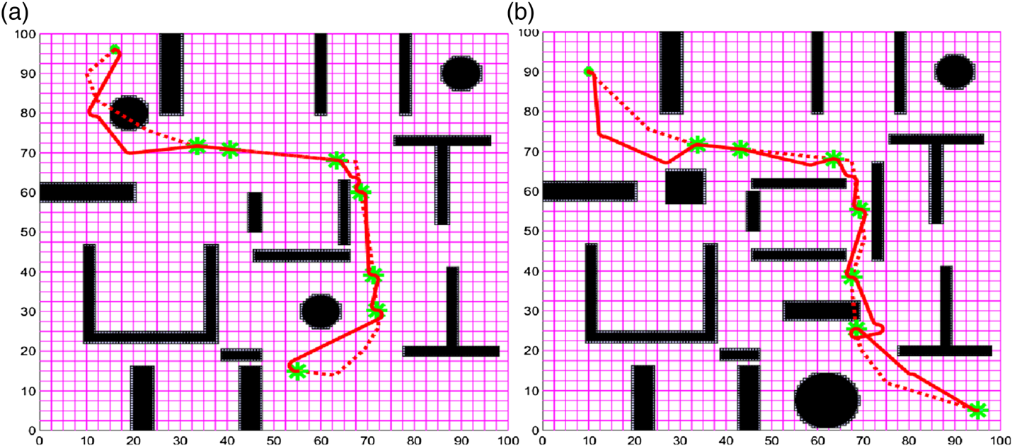
Figure 11. Monte Carlo experiments with changing ending nodes and obstacles.
We embedded the DDRRT* method in a distributed hardware-in-the-loop USV motion simulation platform and conducted extra simulations to demonstrate the applicability and effectiveness of the DDRRT* in dynamic obstacle avoidance scenarios. We choose this platform because it is similar to a practical USV OPP system and enables the presentation of the OPP process by three-dimensional animation. The platform is created on a PC-104 development board, and the OS and development environment are VxWorks 6.6 and Workbench 3.0 (developed by the Wind River Company).
The motion control and navigation data feedback processes are done on the visual simulator. The communication between the PC-104 and the visual simulation computer is realised by a socket program in accordance with the UDP protocol in the broadcast style, because the packet dropout and time delay problems exist and only the latest data are utilised.
Different dynamic obstacle avoidance scenarios are shown in Figure 12(a)–12(d). The dynamic obstacle ability of DDRRT* based on the collision cone estimation and COLREGs regulation is thus demonstrated. The currents, waves and cluttered and dense islands are considered in the practical ocean environment. The platform uses the proportional-integral-derivative (PID) algorithm to control the direction of the USV and the pole placement method to manage the USV's linear speed. The DDRRT* algorithm can provide stable low-cost and low-collision-risk paths.

Figure 12. Dynamic obstacle avoidance path planning process: (a) collision avoidance for the head-on situation, (b) collision avoidance for the overtaking situation, (c) crossover dynamic obstacle from right, (d) crossover dynamic obstacle from left.
5. CONCLUSION
An OPP system based on the RRT* method is proposed for efficiently planning and refining local paths in practical marine environments under USV motion constraints. This system mainly combines selection of subgoals, proportional navigation guidance-based heuristic sampling, and marine environmental information-based sampling space reduction schemes. Sampling space reduction is utilised in accordance with DDRRT while considering disturbance from currents and waves and obstacle avoidance problems. Our DDRRT* method can alleviate the problems of the IRRT* algorithm, such as slow convergence, roughness of sampling space reduction, and lagging of sampling space adjustment. Meanwhile, the heuristic sampling method is used to guide the planner in better utilising the knowledge provided by the global path, and generate more feasible paths. Experimental results demonstrate that the DDRRT* method plans lower-cost paths with effective energy saving of the downstream parts using the drive from currents and waves, and smaller lateral deviation interference from them, than using traditional techniques. Moreover, the refinement of the DDRRT* method is more stable and efficient than that of traditional ones in the environment. Finally, the dynamic obstacle avoidance ability of DDRRT*, based on the collision cone estimation and COLREGs, is also demonstrated in this study. The layered OPP framework is proved to be practical.
This work promotes the study of USV coordination, which is the future direction of the authors' research. Meanwhile, much work remains to be done to achieve the aim of practical USV automation and intelligence, such as the interaction of humans with USVs, intelligent decision making driven by events, accurate prediction according to a more precise motion model and path searching in a smaller parameter range, and the usage of currents and waves to save energy.


