1. INTRODUCTION
Since their first development, the military community has shown interest in Unmanned Surface Vehicles (USVs) for their deployment in force protection and surveillance scenarios (Bertram, Reference Bertram2008). Other examples include the Spartan produced by the US Space and Naval Warfare System Center (SSC) in San Diego, the Delfim developed by the Portuguese Dynamical Systems and Ocean Robotics (DSOR) Laboratory (Alves et al., Reference Alves, Oliveira, Oliveira, Pascoal, Rufino, Sebastiao and Silvestre2006), and the Springer developed by Plymouth University (Naeem and Sutton, Reference Naeem and Sutton2009). Most of the vessels are dual-purpose vehicles, i.e. they can both be controlled remotely and operated autonomously.
USVs usually adopt catamaran and kayak shapes, for their roll robustness or ease of manufacture, and they are generally provided with a rudder-propeller system for propulsion and steering. Their kinematics are modelled ignoring pitch and roll, and considering an Earth-fixed frame and a body-fixed one (Bibuli et al., Reference Bibuli, Bruzzone, Caccia and Lapierre2009). The first is used to express the position and the orientation [x y z] T , while the second is used for surge u r and sway velocities v r relative to the water, yaw rate r and forces and moments. Linear and angular velocities are defined by the following equations, expressed in the Earth-fixed frame:
 $$\left\{\matrix{\acute{x} =u_{r}cos\omega -v_{r}sin\omega +\acute{x}_{c} \hfill \cr \acute{y}=u_{r}sin\omega +v_{r}cosw+\acute{y}_{c} \hfill \cr \acute{\omega}=r \hfill \cr}\right. $$
where
 $\lsqb \acute{x}_{c}\ \acute{y}_{c}\rsqb ^{T}$
are the sea currents that are considered constant, although in general, the marine environment introduces a number of serious disturbances which affect the control of a USV (Bandyophadyay et al., Reference Bandyophadyay, Sarcione and Hover2010). Examples are sea currents, tides, and sea-bed conformation. When transiting close to the coasts, the presence of tides dictates where a ship can go and how much time it will take to reach its destination. Despite the importance of weather conditions while traversing, there are only a small number of papers addressing this issue.
$\lsqb \acute{x}_{c}\ \acute{y}_{c}\rsqb ^{T}$
are the sea currents that are considered constant, although in general, the marine environment introduces a number of serious disturbances which affect the control of a USV (Bandyophadyay et al., Reference Bandyophadyay, Sarcione and Hover2010). Examples are sea currents, tides, and sea-bed conformation. When transiting close to the coasts, the presence of tides dictates where a ship can go and how much time it will take to reach its destination. Despite the importance of weather conditions while traversing, there are only a small number of papers addressing this issue.
The existence of an obstacle detection and avoidance module requires combining the sensing and decision making components, as shown in Figure 1 to navigate autonomously (Statheros et al., Reference Statheros, Howells and McDonald-Maier2008; Tam et al., Reference Tam, Bucknall and Greig2009; Hasegawa and Kouzuki, Reference Hasegawa and Kouzuki1987; Hasegawa; Reference Hasegawa2009). The path planning problem has a long history in robotics, especially for Unmanned Ground Vehicles (UGVs) (Fahimi, Reference Fahimi2008). A Path Planner (PP) is generally composed of a global path planner and a local one. The first (deliberative) must find a safe path connecting the actual position of the robot and its destination. The local (reactive) must react to immediate collisions, moving the vehicle on a different route. Referring to unmanned boats, obstacles are represented by other vessels, divers, buoys, rocks, harbours, islands and coasts.

Figure 1. Architecture of an autonomous system.
The sensing module covers a key role towards full autonomy since it must identify the surrounding obstacles. When static, finding a safe path is easy and any graph search algorithm can be used. However, detecting collisions in time is still an open problem because of sensor limitations (e.g., false positive/negative due to noisy data). Moreover, the conformation of the environment can occlude the sensor's field of view, preventing a moving obstacle's detection. Therefore, autonomous navigation is a more complex task than connecting two points; multiple situations must be considered, especially under uncertainty. Hence, the scope of this paper is to offer an overview concerning the latest methods regarding collision avoidance for USVs and how to solve the problems described above.
This review is divided in the following way: Section 2 illustrates how to perceive the surrounding environment; in Section 3 the necessity of having a robust path planner is discussed, focusing on the difference between global and local path planners, and introducing intelligent methods. Finally, in Section 4, concluding remarks are given.
2. COLLISION DETECTION
To avoid obstacles, an accurate representation of the environment is required. To obtain it, data from sensors (often integrated with electronic charts) are combined to give a Two-Dimensional (2D)/Three-Dimensional (3D) model.
With regards to technology advancements, the methods for collision identification have dramatically changed in the last fifty years (Kemp et al., Reference Kemp, Bechley, Cockcroft, Jurdzinski and Thirslund2012) and sensor advantages and limitations are summarised in Table 1.
Table 1. Advantages and limitation of various sensors within USVs (Liu et al., Reference Liu, Zhang, Yu and Yuan2016).

In Almeida et al. (Reference Almeida, Franco, Ferreira, Martins, Santos, Almeida and Silva2009) a radar classifies targets in terms of a collision threat. A set of perimeters (Figure 2) is defined around the USV: irrelevant (3 km), safe (500 m), warning (250 m) and prohibition perimeter (50 m). Based on the Closest Point of Approach (CPA), the estimated shortest distance between the detected object and the USV, targets are classified as no threat, low threat, potential threat and dangerous. Low-cost radars are also used in Schuster et al. (Reference Schuster, Blaich and Reuter2014) to compensate for the lack of an automatic identification system. Despite the fact that radar has been extensively used for far-field obstacle detection, its accuracy is low for short distances. It is then difficult to detect changes in course in time. Moreover, high waves and water reflectivity still represent a major challenge.
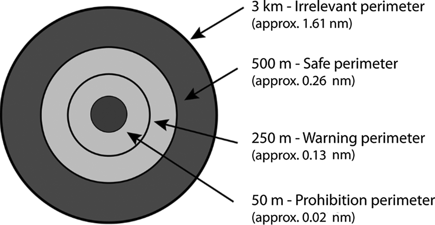
Figure 2. The proximity of the USV (Almeida et al., Reference Almeida, Franco, Ferreira, Martins, Santos, Almeida and Silva2009).
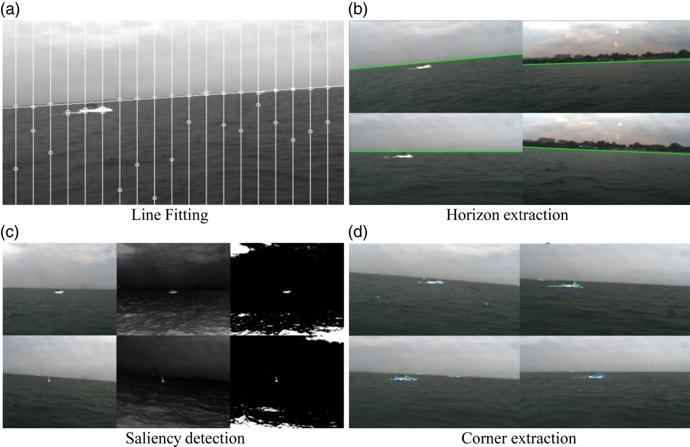
Other approaches use vision methods for recording obstacles near the vessel. For example, Wang et al. (Reference Wang, Wei, Wang, Ow, Ho and Feng2011; Reference Wang, Wei, Ow, Ho, Feng and Huang2012) use two parallel cameras. In the first monocular phase, the horizon is extracted using the Random Sample Consensus (RANSAC) (Fischler and Bolles, Reference Fischler and Bolles1981) method (Figure 3(a)), a binary mask is built (Achanta et al., Reference Achanta, Hemami, Estrada and Susstrunk2009) and detected salient features are considered of potential interest (Figure 3(c)). Surface obstacles are distinguished (Harris and Stephens, Reference Harris and Stephens1988; Bouguet, Reference Bouguet2000) (Figure 3(d)) and interesting ones are tracked in consecutive frames to validate them as potential obstacles (Figure 4). Stereo correspondence was then realised applying an epipolar constraint to reduce the search space. This approach showed good results up to 100 m from the USV using a low-resolution image. Monocular greyscale images are used in Azzabi et al. (Reference Azzabi, Amor and Nejim2014). The Sobel operator and the Hough transform are applied to extract the edges (Maini and Aggarwal, Reference Maini and Aggarwal2009; Hough, Reference Hough1962), then the horizon is identified and moving objects are detected using optical flow estimation. Finally, the distance to obstacles is estimated using geometric relationships (Figure 5). Using greyscale images, the authors reduce the computational effort required by other algorithms (e.g., Ettinger et al., Reference Ettinger, Nechyba, Ifju and Waszak2003).

Figure 3. Monocular obstacle detection (Wang et al., Reference Wang, Wei, Wang, Ow, Ho and Feng2011; Reference Wang, Wei, Ow, Ho, Feng and Huang2012).

Figure 4. The obstacle is tracked between successive frames (Wang et al., Reference Wang, Wei, Wang, Ow, Ho and Feng2011; Reference Wang, Wei, Ow, Ho, Feng and Huang2012).

Figure 5. Estimation of the USV-obstacle distance (Azzabi et al., Reference Azzabi, Amor and Nejim2014).
Other systems use Infra-Red (IR) cameras due to their ability to discretise temperatures. The main advantage of IR cameras is the possibility to overcome the impact of various light conditions (darkness or fog), allowing operations in day and night to take place with little deterioration in performance. In Borghgraef et al. (Reference Borghgraef, Barnich, Lapierre, Van Droogenbroeck, Philips and Acheroy2010), floating mines were identified in the Persian Gulf. Two background subtraction algorithms, the Visual Background extractor (ViBe) (Barnich and Droogenbroeck, Reference Barnich and Van Droogenbroeck2011) and the behavioural subtraction (Jodoin et al., Reference Jodoin, Konrad and Saligrama2008), were implemented. Without specifying any details about the target object, this approach detects every anomaly in respect to the background. IR data are also used in Park and Jeong (Reference Park and Jeong2012), where a multi-step algorithm extracts the shape of a floating object. Vertical and horizontal edges are initially extracted to find candidate objects. Then, the background is removed and a logical AND operation with the original frame is performed to highlight the object region. The limit shown by the previous approaches relies on detecting small obstacles at long distances but, unfortunately, IR applications are still very limited. For this reason, it has not been proved that marine situations such as sea fogs, wave occlusions, variations of lighting and weather, and object reflections do not affect IR cameras' performances like common video cameras (Liu et al., Reference Liu, Zhang, Yu and Yuan2016).
From the consolidated use with an UGV, Lebbad and Nataraj (Reference Lebbad and Nataraj2015) adopt a LIDAR (Laser Direction and Ranging) because a laser entering the water dissipates itself, segmenting any object present there. Sensor data are combined with that of a camera and the object area is then identified. The authors discovered that the vessel's motion can distort the LIDAR image and some of the targets may appear tilted. A similar approach was proposed in Halterman and Bruch (Reference Halterman and Bruch2010) where sensor data were analysed with regards to different parameters (i.e., scanning rate and density, coverage in azimuth, elevation and range etc.). It was noticed that most of the obstacles appear clearly in the returned data while the sea surface does not provide any return. On the other hand, problems are posed by the presence of salt spray, winds, waves, currents and tides that produce image blurring and vibrations (Gal and Zeitouni, Reference Gal and Zeitouni2013).
3. PATH PLANNER
After perception, a representation of the world is realised. This can be done in a 2D or 3D space but the first option is often preferred because it is less computationally demanding (even though the depth dimension can also be useful for navigation purposes). As stated in Section 1, the Path Planner (PP) is usually subdivided: the global PP identifies a free path from the actual position of the robot to a destination, while the local PP tries to avoid close moving obstacles.
In the following subsections, the most recent techniques used in marine robotics are described. Before that, certain navigation rules are introduced.
3.1. The International regulations for avoiding collisions at sea
While underway, vessels must obey rules designed to avoid any kind of collision. Despite being manned or not, the rules must be obeyed by any kind of vessel operating at sea (Wilson et al., Reference Wilson, Harris and Hong2003; Lee et al., Reference Lee, Kwon and Joh2004; Kemp, Reference Kemp2002; Belcher, Reference Belcher2002). Differing, confused behaviour can lead to collisions with other marine craft. The COLREGS (COLREGS, 1972) an abbreviation for the International Regulations for Preventing Collisions at Sea, are divided into three parts. Part A defines vessel and authority responsibilities, Part B regulates the conduct of vessels in an encounter, and Part C establishes communication protocols. Rules contained in Part B are defined as Steering and Sailing Rules, and the more important are reported in Table 2.
Table 2. Selected Rules from the International regulations for avoiding collisions at sea (COLREGS, 1972).
The rapid increase in the number of USVs posed interesting questions about their responsibilities while underway (Allen, Reference Allen2012). This is still an open problem, the US Navigation Safety Advisory Council seems inclined to recognise their status as ‘vessels’ and, therefore, their obligations in an encounter.
3.2. Global path planner
A global path planner must continuously adapt the existing path to new long-range obstacles. Larson et al. (Reference Larson, Bruch, Ebken, Warfare, Diego and Diego2007a; Reference Larson, Bruch, Halterman, Rogers and Webster2007b) discretise the environment in a bi-dimensional grid. Stationary obstacles are provided by a chart server, and moving ones by the radar. The A* algorithm (Hart et al., Reference Hart, Nilsson and Raphael1968) was chosen as the search technique and a proximity cost added to prevent the USV going close to obstacles. To avoid the moving ones, safe velocity ranges are determined using the Velocity Obstacles (VO) method (Figure 6): a velocity space v-θ grid (where v identifies the vehicle's speed and θ its heading angle) is built where the obstacle's size is increased and the robot treated as a point. To avoid any collision, the robot's velocity must lie outside the VO. If a collision cannot be avoided, a Projected Obstacle Area (POA) (Figure 7), the future occupied area, is created for each obstacle and a new safe route is found. The authors also implemented the COLREGS, in particular rules 13, 14 and 15.

Figure 6. To avoid the collision, the relative velocity vA - vB must be outside the cone defined by the USV centre and the expanded obstacle (Larson et al., Reference Larson, Bruch, Ebken, Warfare, Diego and Diego2007a; Reference Larson, Bruch, Halterman, Rogers and Webster2007b).

Figure 7. The projected obstacle area of a moving obstacle (Larson et al., Reference Larson, Bruch, Ebken, Warfare, Diego and Diego2007a; Reference Larson, Bruch, Halterman, Rogers and Webster2007b).

Figure 8. Manoeuvres defined for addressing overtaking (a), meeting (b), and crossing (c) obstacle (Larson et al., Reference Larson, Bruch, Ebken, Warfare, Diego and Diego2007a; Reference Larson, Bruch, Halterman, Rogers and Webster2007b).
Casalino et al. (Reference Casalino, Turetta and Simetti2009) suggest an approach based on the Visibility Graph (VG) concept (Figure 9): for each couple of inter-visible points, a straight line connecting them and not passing into an obstacle was drawn. After transforming obstacles into polygons, the VG is built and Dijkstra's Algorithm (Dijkstra, Reference Dijkstra1959) was applied to find a safe path.

Figure 9. A visibility graph (Casalino et al., Reference Casalino, Turetta and Simetti2009).
A different solution has been proposed by Xie et al. (Reference Xie, Wu, Peng, Luo, Qu, Li and Gu2014) who modified the Artificial Potential Field (APF) (Khatib, Reference Khatib1985) method (Figure 10) in a way that, in the presence of an obstacle, attractions decrease as a linear function and repulsions as a higher-order function. Chen et al. (Reference Chen, Pan, Guo, Huang and Wu2013) propose to adapt the scanning angle of a sonar to the distance from the obstacle using fuzzy logic to make the strategy timely and effective.

Figure 10. The APF model.
Four scan range levels are defined: if no obstacle is detected in a cycle, the scan range will jump to the upper level, otherwise, it will move down to the nearest level bigger than the distance existing between the sonar mounted on the vessel and the identified obstacle. At this point, the type of the obstacle is determined and the slope is calculated. The only limitation is given by the low precision of the Inertial Measurement Unit (IMU) used, which compromised the reaction accuracy.
Chang et al. (Reference Chang, Jan and Parberry2003) extended the maze routing algorithm developed by Lee (Reference Lee1961) to general λ -geometry for λ≥ 4. A route is defined as a data structure composed of the vessel path, the source cell, the destination cell and the speed. The vessel path is a list of all the cells traversed, characterised by their coordinates, the arrival time, and a link to the next one. Unfortunately, the shortest path on a raster grid is not always the optimal one since it could contain too many course alterations. Moreover, a change in speed often corresponds to a longer passage time. This problem has been addressed by Szlapczynski (Reference Szlapczynski2006), which found the shortest path with bend penalisations. The data structure of the previous work is modified to account for the cost of all course alterations.
3.3. Local path planner
One example of a local path planner is given by Kuwata et al. (Reference Kuwata, Wolf, Zarzhitsky and Huntsberger2014), where the COLREGS and VO are considered. Initially, the CPA for every obstacle was calculated and the most suitable rule is applied. A cost for every velocity vj and heading angle θ j admissible was generated and the (vj, θ j) pair with the minimum cost sent to the controller. Similarly, Leng et al. (Reference Leng, Liu and Xu2013) integrated VO with mixed linear integer programming after linearizing the USV's properties, sensor data and uncertainty about the environment. The collision risk is checked by calculating the CPA and its distance from the vessel.
In Larson et al. (Reference Larson, Bruch, Ebken, Warfare, Diego and Diego2007a; Reference Larson, Bruch, Halterman, Rogers and Webster2007b) the Morphin algorithm (Simmons and Henriksen, Reference Simmons and Henriksen1996) is applied, drawing multiple arcs in front of the vehicle over the local occupancy map. Thus, all the safe paths are considered, covering every free cell of the map with at least one arc. A weight is assigned to each arc depending on its vicinity to obstacles. The votes are then scaled from 0 to −1 and combined with those coming from other navigation behaviours.
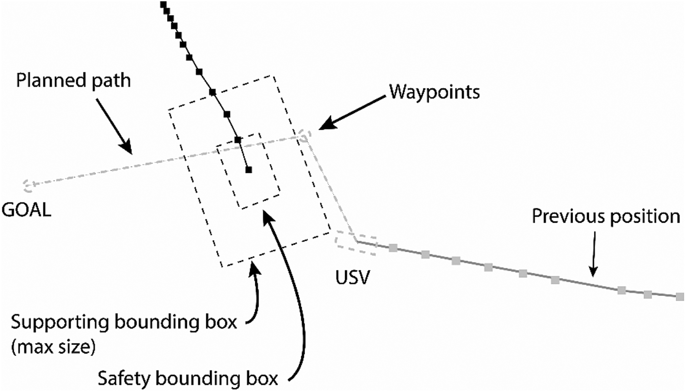
Casalino et al. (Reference Casalino, Turetta and Simetti2009) describe a method based on the Bounding Box (BB) concept, defined as the rectangular area the vessel should avoid. The algorithm integrates the BB vertices with the vehicle position S and the goal G into a graph. The solution is any path from S to G, identified using A*. Since kinematic constraints are neglected, the work suffers from sub-optimality. In successive work (Simetti et al., Reference Simetti, Torelli, Casalino and Turetta2014), a safety BB is added and all the computations are now performed against it; after entering the safety box, the USV must leave it without intercepting the main diagonals and ensuring in this way the collision BB is not crossed. To address uncertainty, a supporting BB is adopted (Figure 11), whose dimensions may vary from coinciding with the safety one's to be identical to the maximum bounding box's. Thus, the path's robustness to changes in speed and heading of the obstacle is increased.

Figure 11. The bounding boxes of a moving obstacle (Simetti et al., Reference Simetti, Torelli, Casalino and Turetta2014).
An approach based on lane-constrained trajectory is proposed in Tan et al. (Reference Tan, Wee and Tan2010). Here, while avoiding obstacles, the vessel must meet several objectives such as maintaining a minimum distance from each obstacle, respecting the COLREGs, keeping as close as possible to the intended path and complete the trajectory in the shortest time possible. Initially, the platform's motion is forward simulated for a fixed number of time steps using simple models of a manoeuvre tracker and the vessel. Then, objectives are ordered and an elimination multi-stage process takes place. Regrettably, the algorithm may sometimes be unable to find a solution since only a sample of possible manoeuvres is generated.
Blaich et al. (Reference Blaich, Koehler, Schuster, Reuter and Tietz2015) modified the A* algorithm to allow velocity variations and different turning circles. The cost function is adapted adding a penalty representing the amount of path skipped during the evasion manoeuvre. In this way, the USV is led back to the original path after the deviation. Velocity and time are added to the search space to guarantee the feasibility of the trajectory.
Tang et al. (Reference Tang, Zhang, Liu, Zou and Shi2012) developed a new method called Obstacle Avoidance Algorithm Based on a Heading Window (OAABHW). To obtain the best navigation angle θ out, the heading yaw, is considered as an optimisation objective, with the heading window and the set of unfeasible heading angles as constraints. From θ out and the current heading angle θUSV, it is possible to obtain the avoidance rotational velocity ωout. Zhang et al. (Reference Zhang, Tang, Su, Li, Yang and Shi2014) illustrated a new adaptive collision avoidance algorithm based on State-Action-Reward-State-Action (SARSA) on-policy reinforcement learning (Sutton and Barto, Reference Sutton and Barto1998) to face a changing trajectory due to external conditions. It is composed of two modules: the Local Obstacle Avoidance Module (LOAM) and an Adaptive Learning Module (ALM). LOAM focuses on the avoidance manoeuvre, ignoring external disturbance factors, dealt with instead by ALM while searching for a course compensation angle. LOAM calculates the guidance angle with OAABHW, which is forwarded as input to the ALM together with sea winds and currents.
3.4. Intelligent path planner
Differing from the deterministic methods proposed before, some research groups have developed intelligent algorithms based on Fuzzy Logic (FL), Evolutionary Algorithms (EAs) and Artificial Neural Networks (ANNs). These optimisation approaches offer multiple advantages such as lower computation effort and the ability to learn the near-optimal solution. On the other hand, they can fail by getting trapped in local minima or fail to find a solution at all. To overcome these problems, they are often combined in ‘hybrid systems’ (Campbell et al., Reference Campbell, Naeem and Irwin2012).
Hwang (Reference Hwang2002) used a knowledge base and an inference fuzzy engine. Adopting a circular ship domain, the author solves a multi-ship collision one by one, suggesting the manoeuvres as a visual aid or sends them to an autopilot. Liu et al. (Reference Liu, Du and Yang2006) coupled FL with an ANN in a three module algorithm. The first module classifies the collision risk given CPA, course, and distance of the incoming vessel and provides an avoidance manoeuvre. The second calculates the membership function of the speed ratio. The last one generates magnitude and action time. Kao et al. (Reference Kao, Lee, Chang and Ko2007) addressed port navigation safety using FL to calculate a Guarding Ring (GR) and a Danger Index (DI). The radius of the GR is established starting from the length of the ship, its speed, and the sea state. When two GRs start to overlap, the collision alert system is activated. Perera et al. (Reference Perera, Carvalho and Guedes Soares2012; Reference Perera, Ferrari, Santos, Hinostroza and Guedes Soares2015) and Lee and Kim (Reference Lee and Kim2004) provide an example where FL has been combined with a Bayesian network and an APF, respectively.
EAs are heuristic approaches developed to find a close-to-optimal solution in large search spaces. They follow the Darwinian principle that only the best elements of every generation survive a process of variation and selection (Glick and Kohn, Reference Glick and Kohn1996). Smierzchalski (Reference Smierzchalski1999) and Smierzchalski and Michalewicz (Reference Smierzchalski and Michalewicz2000) use genetic mutation operations to modify a ship's speed. COLREGS and the time variable are incorporated during the generation of a new population of trajectories and the solution is searched based on a cost function combining space, time and smoothness. In this model, based on Ito et al. (Reference Ito, Zhnng and Yoshida1999), each chromosome has a different number of genes representing the coordinates of the turning points, the ship's speed, and the interconnections among genes of the same chromosome. A more realistic approach is explained by Zeng (Reference Zeng2003), where a single gene is characterised by some noise parameters, such as wind, wave and sea current. The length of each chromosome depends on the navigation (Figure 12). The same approach is also used by Tsou (Reference Tsou2010). The selection of the best route is made using the roulette selection method, after ordering all of them per a linear fitness function. In Szlapczynski (Reference Szlapczynski2013; Reference Szlapczynski2015), evolutionary algorithms were used to find a set of safe trajectories for all ships involved in a collision. Six types of violations were identified and corresponding penalties introduced. Ship tracks, modified in course and speed, are therefore evaluated with a fitness function inversely proportional to penalties.
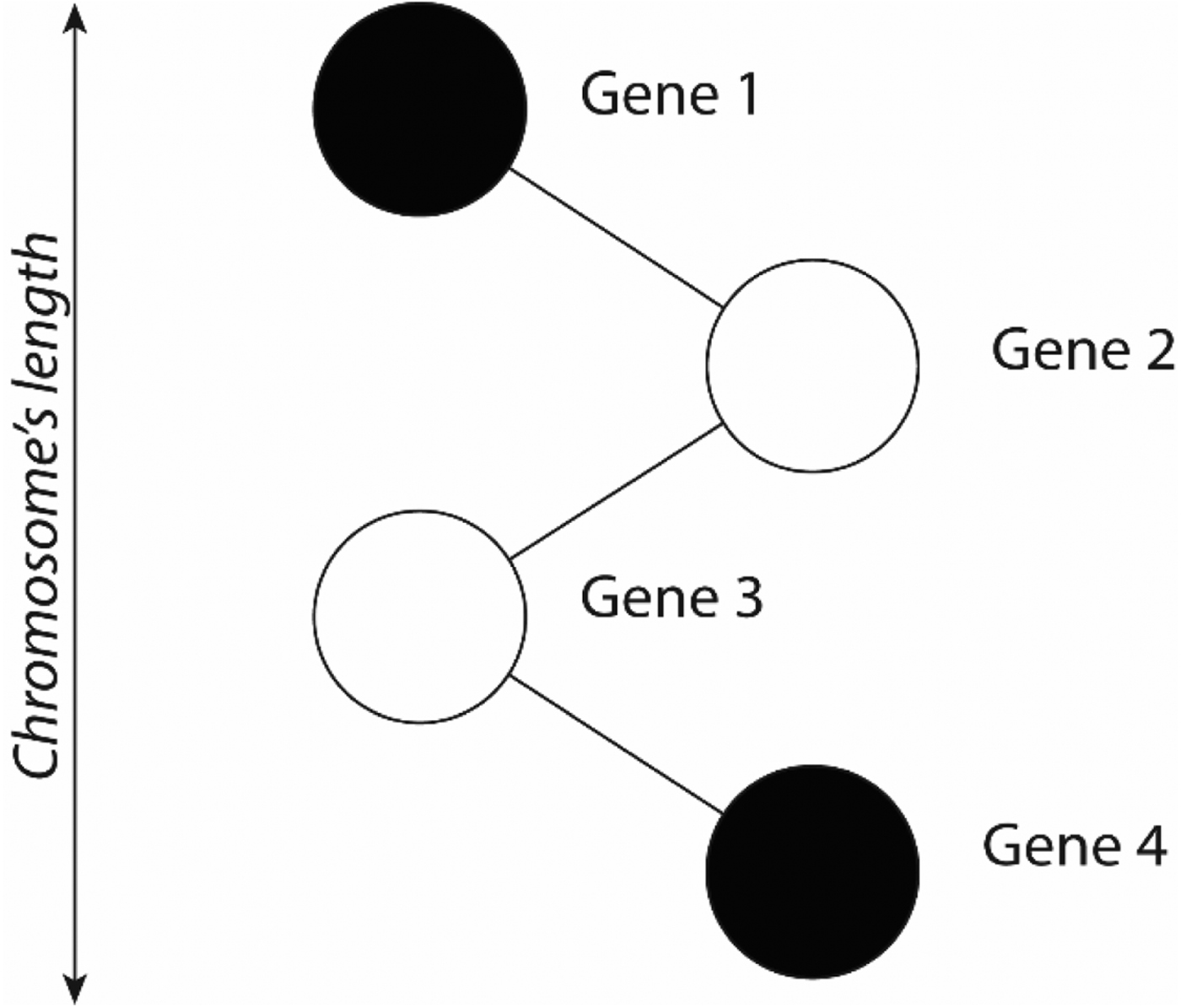
Figure 12. The route as a chromosome.
In contrast, in Lazarowska (Reference Lazarowska2015) the path planning problem is solved as an Ant Colony Optimisation (ACO) problem. ACO is inspired by the indirect communication mechanism observed among ants.
A graph considering all the constraints and the ship position is built. At this point, every ant constructs its path from the starting vertex until the ending one: at each step, the ant chooses its next position based on the value of the pheromone trail. After all the ants complete the task, the pheromone trail is updated penalising those vertices with a constant value and increasing the others. The algorithm terminates when a maximum number of iterations is reached or after a maximum computational time. The path selected is shown to be the shortest.
4. CONCLUDING REMARKS
The review presented in this paper began by comparing different sensors employed for acquiring information about the environment. Classic sensors used in the marine environment such as sonar and radar, as well as those mounted on a ground vehicle, i.e. cameras and LIDARs, have been evaluated to establish how good they are in identifying static and moving obstacles. Studies involving them are reported and their respective advantages and drawbacks have been shown. It is concluded that the radar, despite being the sensor most used for preventing a collision at sea in the past, suffers from a lack of accuracy while trying to identify objects at close distance. Vision-based (mono and stereo) approaches can achieve better results than radar despite maritime phenomena like lightning changes and waves still posing a big challenge in the field. Infra-red cameras can offer a partial solution to the previous problems but only a few works have employed them thus far. Many efforts have been made to adopt the use of LIDAR from unmanned ground vehicles but, despite calibration problems now being solved, the same issues for visual sensors still hold. Therefore, it is possible to conclude that the obstacle detection problem remains open and a definitive robust solution is still missing.
Multiple path planners have been reported, classifying them as global or local ones. A stand-alone section has been dedicated to the so-called ‘intelligent’ methods, based on soft computing techniques. ANNs have been applied to this problem due to their nonlinear mapping, learning ability and parallel processing. Fuzzy logic, instead, can simulate the human thinking represented by knowledge-based conditional rules. All the methods described must face the difficulty of addressing complex encounter scenarios that would require human-like experience to choose the best action. Considering that most of the time they work as a black-box (e.g., ANN), the convergence to the optimal solution is not guaranteed. In addition, these techniques are computationally time-consuming. Therefore, they should be discarded while considering real-time navigation but they can be adopted in different tasks where they have already proved to be efficient (e.g., convolutional neural networks for identifying possible obstacles in front of the vehicle). A major problem with most of the solutions reported is that they have been tested only in simulation while proving their validity in the real world still has to be done. Moreover, their reliability is limited by the results that can be incomplete due to a small subset of scenarios tested, or small for a proper probabilistic analysis (Niu et al., Reference Niu, Lu, Savvaris and Tsourdos2016). It is therefore plausible to affirm that there is no guarantee in avoiding obstacles in all conditions with the methods above. In addition, three serious shortfalls have been identified:
-
• while defining the path, most of the methods reported do not consider the vessel's dynamics;
-
• others ignore the COLREGS despite this being a mandatory requirement while underway in open waters;
-
• almost all of them do not take in account weather and sea conditions.
Taking these points in order, most of the path planners previously described produce unexecutable paths. Treating the USV as a point and ignoring its dynamics (e.g., the minimum turning radius of the vehicle), they generate way-point paths in which two points are generally connected by a straight line. This results in a trajectory characterised by high turning rates with the possibility of damage to the vessel's actuators. To avoid this problem, the solution is to incorporate the vessel's dynamics (in terms of velocity, drag and heading angle) within a cost function in the formulation of the path to making it suitable for the USV's turning abilities.
The second main point to address is the implementation of the COLREGS. This is an important requirement for all types of USVs since they must show an intelligent behaviour for understanding and executing the standard rules for marine navigation. There is not a universally agreed solution to incorporate them and most of the existing works either disregard them or adopt different safety domains to emulate them. In a few cases, they are included in the solution space but the optimality is not guaranteed. Therefore, to simplify the decision-making process in an encounter, it has been decided that an autonomous vessel always has to give away if a doubt arises while meeting a manned vehicle.
Finally, future work should address environmental disturbances and uncertainties. USV path planning is dependent on the combined effect of wind, waves and currents, where wind and wave effects can be neglected for larger vessels (Lee at al., Reference Lee, Kim, Chung, Bang and Myung2015). High speed currents can deviate the vehicle from the planned path instead. The incorporation of such environmental effects within the planning process, while improving the overall understanding of the surrounding world increases the computational complexity for the optimal path planners. In the same way, varying environmental conditions (e.g, fog, lighting, rain, wave occlusions, sophisticated background) as variations in the view angle and range, still represent an issue for real-time vision-based perception.