2.1. Overview

The functional architecture of the method used in Konno et al (Reference Konno2006a, Reference Konno2006b) to mitigate the risks induced by the ionosphere is shown in Figure 2. The method is essentially divided into two parts:

• • mitigation under nominal conditions using the DFree and IFree methods to reduce the overall uncertainty introduced by the ionosphere (under the assumption that the state of the ionosphere is known – i.e. that monitors exist), and

• • monitoring of the ionosphere to exclude affected satellites and compute protection levels under non-nominal ionosphere conditions.

Figure 2. Functional architecture of Ionosphere monitoring in (Konno et al., Reference Konno2006a, Reference Konnob) measurement observables.

The dual-frequency observables used by Konno et al. (Reference Konno2006b) in determining the ranges is based on the use of divergence-free (DFree) and ionosphere-free (IFree) smoothing. The objective of smoothing is to minimise the noise on the code measurements using the less noisy carrier-phase measurements.

DFree removes the temporal gradients from the ionospheric delay using dual frequency carrier phase measurements to smooth the code measurements. However, spatial ionospheric gradients are not removed with the DFree method. Therefore, Konno et al. (Reference Konno2006b) propose an alternative method, IFree smoothing, which removes the spatial and temporal effects using linear combinations of dual-frequency code and carrier measurements. However, the method suffers from noisy outputs from the smoothing filter, resulting in reduced availability. Therefore, the optimal choice of the smoothing method depends on the state of the ionosphere. Under nominal conditions, Konno et al. (Reference Konno2006b) show that DFree smoothing leads to a higher availability. Conversely, under strong ionosphere anomaly conditions the IFree provides a higher availability, only limited by the receiver error models and the alert limits. In order to optimally combine these two smoothing algorithms, a monitor is needed to track the state of the ionosphere and provide an alert to switch between the DFree and IFree smoothing methods.

The relevant results obtained in Konno et al. (Reference Konno2006b) are summarized as follows:

• • The DFree algorithm, under nominal ionosphere conditions, reaches an availability of 98·7% if a VAL=5·3 m is assumed. This is below the minimum availability requirements of 99·9% for CAT-III approaches. A VAL=2·6 m (as specified by EUROCAE, 2007) would lower this further.

• • The IFree algorithm, with improved Airborne Accuracy Designator B (AAD-B) and Ground-Accuracy Designator C (GAD-C) error properties, by 75% and 50% respectively, produces a maximum availability of 98·4% with a VAL=5·3 m. Again, a VAL=2·6 m will result in a lower availability.

In order to determine the state of the ionosphere and choose the appropriate smoothing method, Konno et al. (Reference Konno2006a) propose a monitoring architecture (depicted in Figure 2) and described in the next Section.

2.2. Ionosphere Monitoring

Konno et al. (Reference Konno2006a) propose two ionosphere monitors based upon measurements of the temporal and spatial gradients of the ionosphere delays at both the GGS and the user locations: rate-based and delay-based monitors. In the former, the temporal gradients are computed using dual-frequency carrier-phase measurements and are then converted to spatial gradients making the assumption that ionosphere fronts can be modelled in terms of a gradient, a width and a velocity. The drawback is that if the Ionosphere Pierce Point (IPP) moves with the same velocity as the ionosphere front, no time variations and hence no spatial variations are detected. To compensate for this undetectable condition, Konno et al. (Reference Konno2006a) introduce the delay-based algorithm that directly computes the ionosphere spatial differences using dual frequency code measurements. These are double differenced, to remove the Inter-Frequency Bias (IFB), and carrier-phase-smoothed, to reduce the noise. The assumption is made that both the user and the GGS have the same ionosphere monitor.

The rate-based monitor estimates temporal gradients using dual-frequency carrier-phase measurements. As identified in Konno et al. (Reference Konno2006a), a potentially hazardous situation occurs when the front and IPP velocities align, making it impossible for the rate-based ionosphere monitor to detect this threat. Konno et al. (Reference Konno2006a) conclude that a front that moves with the IPP of the user and hits the IPP of the GGS just as the user passes the decision point is the most severe undetectable condition with this monitor. This is applicable to fronts affecting any number of satellites, although in practice such alignment has only been observed for up to two satellites. As a result of this deficiency, the delay-based monitor was developed based on the comparison by the user of the ionosphere-induced delays computed and broadcast by the GGS with those computed by the user. However, the approach has the weaknesses of errors from high noise levels and the difference in inter-frequency bias between the GGS and user receivers (the satellite hardware group delay is common to both GGS and user and hence cancels out). The IFB is cancelled out by double differencing with the highest satellite.

2.3. Current Limitations

The method developed in Konno et al. (Reference Konno2006a) combines the rate-based algorithm with the delay-based algorithm to monitor the ionosphere. Theoretically, it allows switching between the DFree user algorithm under nominal ionosphere conditions and the IFree algorithm under ionosphere anomaly conditions. Furthermore, it allows optimisation of service availability by using the satellite exclusion of the monitors as well as the computation of standard and enhanced Vertical Protection Levels (VPLs). However, there are a number of limitations to this approach:

• • The IFree method can only support a Vertical Alert Limit (VAL) larger than ∼10 m if error levels of the GGS and user receivers are improved by up to 75% with respect to current levels, in order to satisfy CAT III minimum service availability requirements (99·9%). In particular, the availability of CAT III approach service with the IFree algorithm with a VAL ∼5·3 m, and assuming current GGS and user receiver error specifications, is at the level of 0·001%. In order to meet the 99·9% availability requirement specified by the RTCA (2004) and EUROCAE (2007), the VAL assumption, which is already larger than the 2·6 m requirement by EUROCAE (2007), would need to be relaxed significantly further. The availability can be shown to increase to 99·977% if the ground errors are improved by 50%, the airborne errors by 75% and the VAL is relaxed to 10 m. In order to be beneficial, significant reduction in receiver errors and relaxation of VAL are required. Whilst the former is likely to be achieved in the future, a relaxation of the VAL is not in line with developments by EUROCAE (2007).

• • The baseline (rate-based monitoring) and enhanced (rate-based and delay-based) systems can only support a VAL of 16·5 m and 14·5 m respectively to reach the CAT III minimum service availability of 99·9% (Konno et al., Reference Konno2006a). This is significantly larger than the VAL=2·6 m proposed by EUROCAE (2007) and also larger than the VAL=10 m proposed by the RTCA.

• • The rate-based monitor algorithm is unable to detect fronts where the satellite IPPs all align with and move at the same velocity as the front. Moreover, the assumption is made that this scenario is limited to two satellites. Although scenarios with more than two satellites have not been observed based on the study results of three cities within the CONtinental United States (CONUS), there is no guarantee that such scenarios do not exist. Additionally, if ionosphere-induced errors for more than two satellites lie under the minimum detection threshold of the rate-based monitor, they are potentially not detected. As a result, it is unclear whether the rate-based monitor is in fact able to limit the affected number of satellites to two.

• • The delay-based monitor suffers from large noise errors and inter-frequency biases. The removal of the latter using double differencing leads to the exclusion of at least two satellites simultaneously, raising questions about the impacts on the continuity of service. Moreover, implications for the comparisons with other satellites need to be carefully addressed.

• • The reliability of ionosphere monitors could be compromised by unknown ionosphere anomalies since a maximum bias of 400 mm/km together with a nominal dispersion of 5 mm/km is currently assumed in the computation of the VPL.

Given the limitations of the methods described above, Section 3 develops a new method, that has the potential to significantly mitigate the risks associated with ionosphere fronts. Whilst a detailed study of the performance of the proposed method is beyond the scope of this paper, a high level analysis of the expected improvements over the current state-of-the-art is given in Section 3.3.

3.1. Functional Architecture

Figure 4 presents the proposed functional architecture for E-GBAS. The introduction of additional monitors into the GBAS architecture serves two purposes: to accurately monitor the ionosphere and to minimise potential decorrelations between aircraft and GGS. Furthermore, it is to provide an overall estimate of the range uncertainty in the corrected data at aircraft level, hence providing additional redundancy, with the potential to increase availability.

Figure 4. E-GBAS monitor functional architecture.

3.1.1. Ionosphere Monitor

The ionosphere monitor directly estimates the ionosphere delays using dual-frequency carrier-phase measurements:

(2)

where:

α=

1−f ₁²/f ₂²

ɸ=

carrier-phase observable

I _1,jⁱ=

ionosphere advance of L1 carrier

τ ₂₁ⁱ=

hardware group delay between L1 & L2 carrier

IFB _21,j=

interfrequency bias between L1 & L2 carrier

Δv _21,jⁱ=

difference in carrier-phase noise and multipath between L1 & L2 carrier

ΔN _21,jⁱ=

difference in carrier-phase ambiguity between L1 & L2 carrier

Since the difference in ionosphere delays between the GGS and the GMs is of interest, the satellite hardware group delay τ ₂₁ disappears:

(3)

Given that the GMs and the GGS are stationary, reliable ambiguity resolution and cycle slip detection can be achieved. The uncertainty in the estimate of the difference in ionosphere delays between the GGS and the GMs is given by:

(4)

The uncertainties associated with the Inter-Frequency Bias (IFB) are of the order of a few millimeters for carrier-phase L1 and L2 (Liu et al, Reference Liu, Tiberius and De Jong2004) and can therefore be neglected. The same applies for a combination of GPS L1 and L5 as well as the corresponding Galileo signals. The uncertainty in the difference in ionosphere-delay estimations is thus essentially determined by the carrier-phase noise and multipath.

The expected ionosphere bias between the GGS and the aircraft as well as the remaining uncertainties can be extrapolated from the individual ionosphere delay measurements at the GMs and the GGS. The bias is corrected for in the positioning algorithm, and the uncertainty used in the computation of the protection levels. An alternative (more conservative method) would be to use the maximum gradient within the coverage area to compute the maximum bias in ionosphere delay between the GGS and the aircraft in the computation of the protection levels.

The VPL at aircraft level is computed from the above ionospheric uncertainties (Equation 4) as well as the remaining uncertainties (troposphere, code noise at aircraft and GGS), adding the maximum bias that could go undetected with the given monitor configuration. Using the DFree configuration of (Konno et al., Reference Konno2006b) to compute the differentially corrected ranges at aircraft level, the corresponding vertical protection level is computed as:

(5)

where K _ffmd is the fault-free detection multiplier determined from the maximum allowable integrity risk. The maximum bias is determined from the maximum gradient of the allocated threat-space and the maximum distance between the aircraft and the closest baseline joining either two GMs or one GM and the GGS:

(6)

In case of a configuration with four GMs as shown in Figure 7 (See Section 3.2.2), this bias would be zero at the decision height for CAT III precision approaches.

3.1.2. Range Monitor

The range monitors serve as an additional safeguard, and have the potential to increase service availability for those cases in which an individual failure mode leads to unavailability as a result of the PL exceeding the alert limit, whilst the overall integrity risk is still met (as a result of the other errors being below their maximum limits). Each GM corrects its own measurements with the differential corrections (corrected for the difference in ionosphere delays between the two stations) provided by the GGS, to extract the corrected range:

(7)

where

=

differentially corrected DFree – smoothed GM n observable

=

DFree – smoothed GM n observable

=

DFree – smoothed GGS observable

=

True distance between GGS and satellite i

=

True distance between GM n and satellite i

=

time-offset of GM n with respect to GGS

=

difference in troposphere delay between GM n and GGS

F=

smoothing factor

=

difference in noise between GM n and GGS

The corrected ranges are compared to the true ranges to the satellite (from the known GM locations). The measured residual errors are compared to the estimated residual errors, computed based upon the measurement noise, multipath, as well as the ionosphere and troposphere uncertainties. Provided that the measured residual errors are smaller than the estimated residual errors, the satellite is considered healthy. Otherwise, the satellite is excluded.

3.2. Physical Architecture

This section discusses considerations and assumptions for building a physical monitoring architecture capable of satisfying the E-GBAS functions described in Section 3.1, for precision approaches and airport surface movement. In the development of the monitor architecture in the following sections, the following assumptions are made on the ionosphere fronts:

• • they can be described by a velocity vector, a gradient (in two dimensions) and a width;

• • they are wider than the GGS to Ground Monitor (GM) distances.

Furthermore, the proposed architecture accounts for performance requirements, operational constraints and cost. From an operational perspective, the proposed architecture must be able to satisfy all performance requirements of CAT III landings and Airport Surface Movement (ASM). Operational constraints, such as masking satellites visible to the monitors by approaching aircraft, or induction of multipath by aircraft at the monitors, must be given due consideration. Finally, it is clear that any architecture will be a trade-off between the performance it can achieve and the costs incurred.

3.2.1. Performance Considerations

The main issue with the current architecture is that decorrelation between the errors at the GGS and at user level pose a significant integrity threat. This should be mitigated by an appropriately designed architecture. Ideally, one would locate a monitor at the Decision Height (DH) of the aircraft on approach and compute the ionosphere induced delay at this monitor as well as the GGS. If neither GGS nor the Ground Monitor (GM) detects any ionosphere anomaly, then there would be no ionosphere integrity risk for the user at the DH either. However, for practical reasons, such an architecture is not viable as aircraft on the approach would constantly mask the satellites in view of the GM. Moreover, multipath from the aircraft would also be expected to significantly impact the operation of the monitors. Therefore, the GM should be offset from the DH. Larger offsets minimise the risks of shadowing and multipath. At the same time however, the larger the offset, the larger the potential decorrelation between the GM ionosphere delay measurements and the ionosphere delays affecting the aircraft. Therefore, there are two trade-offs to be made:

• • Minimum DH to GM distance for best correlation of errors

• • Maximum DH to GM distance for minimum risk of loss of lock (continuity risk) and minimum risk of multipath

Additionally, maximum GM to GGS distances are desirable to optimise the monitoring sensitivity (“lever-arm effect”) of the E-GBAS architecture.

In order to protect against all ionosphere fronts, the architecture should be designed such that it is not possible for a front to affect only the GGS without affecting the GM. This limits the minimum number of GMs needed to two, in order to “cover” the GGS. With such a configuration, the two monitors would have to be placed on opposite sides of the GGS and in one line (see Figure 5). The disadvantage of such a configuration is that the minimum distance between the baseline, connecting GM1 and GM2, and the DH is still relatively large unless the GMs are placed close to the threshold, hence making the GMs prone to masking and multipath by aircraft. Therefore, in order to “cover” (i.e. protect) the GGS and reduce the uncertainties in the decorrelations between the GGS and the user, the minimum configuration should consist of three GMs. The proposed configurations are shown in Figure 6. GM3 could be placed on either side of the runway.

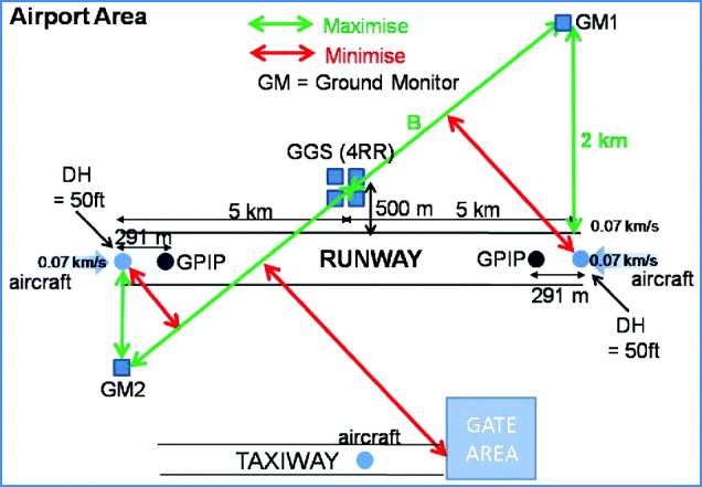
Figure 5. Airport with two GMs.

3.2.2. Operational and Financial Constraints

In order to minimise multipath and masking by aircraft, the GMs should be placed not only sufficiently far from the approach path, but also from the taxiways and buildings. This may suggest that the minimal configuration of Figure 6 may not be sufficient since a larger distance of the GMs to the DH also results in a larger distance between the closest baseline and the DH. As a result, the optimal configuration of such monitor architecture should consist of four GMs, placed such that most of the airport surface is covered, as shown in Figure 7. From a financial perspective, the architecture should be limited to the minimum possible, whilst meeting the operational and environmental constraints.

Figure 6. Airport with three GMs – Proposed minimum configuration.

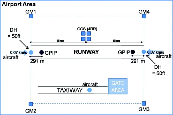
Figure 7. Optimal monitor architecture.

3.3. Expected Performance

A detailed analysis to quantify the performance of the proposed architecture is beyond the scope of this paper. However, a comparison of the residual errors of the method proposed in this paper and the one in Konno et al. (Reference Konno2006a) is presented here. There are several essential differences between the approach that uses the DFree method with the monitoring schemes described in Konno et al. (Reference Konno2006a), and a configuration where DFree is used together with an E-GBAS architecture. Firstly, the E-GBAS architecture is ground based and uses dual frequency carrier-phase measurements, and thus able to very accurately determine the ionospheric delays and uncertainties. Secondly, the first approach suffers from the following main drawback: in order to optimally switch between the DFree and IFree algorithms reliable ionosphere-anomaly monitors are required. Two such monitors to be used in tandem are proposed in Konno et al (Reference Konno2006a). The first, a rate-based algorithm is very sensitive to ionosphere variations, but is not able to reliably detect ionosphere fronts with small differences in speed between the ionosphere pierce point (IPP) and the front. The second monitor is not very sensitive as a result of the relatively large noise levels associated with using double-differenced dual-frequency code measurements, and the need to make various assumptions with respect to maximum potential biases that may be remaining between the GGS and the user. On the other hand, the use of DFree with a suitable E-GBAS architecture configuration is expected to reliably detect all ionosphere fronts with a high degree of sensitivity, and to eliminate the need to make assumptions with respect to potential biases between the aircraft and GGS. It thereby maximises service availability. Thirdly, the E-GBAS architecture provides enhanced availability if used additionally, as a range monitor.

The first two differences suggest that the contribution of the ionosphere-induced uncertainty in the availability computation is expected to be minimal, whilst the third guarantees that any availability comparison is conservative (i.e. the E-GBAS architecture is expected to perform better than a comparison with the DFree/Konno et al (Reference Konno2006a) method would suggest). Comparing for example, the VAL=9·5 m requirement to achieve a 99·9% availability for New York (Konno et al., Reference Konno2006a), an adjustment could be made to the known bias as a result of incorporating E-GBAS to reduce the VAL by ∼4·2 m. The improvement is due to the fact that in the monitoring proposed in Konno et al (Reference Konno2006a), there is a potential residual bias of 4·2 m as a result of potential undetected ionosphere conditions. Using E-GBAS, it is expected that all conditions would be detected, thereby eliminating this bias. This results in a VAL of ∼5·3 m for a 99·9% availability (for GPS dual frequency configurations). Furthermore, considering the fact that Galileo dual frequency configurations are expected to have improved error budgets by at least a factor of two with respect to GPS (Schlueter et al, Reference Schlueter, Bauer and Schuster2005), this would result in an estimated availability of 99·9% for VAL ∼2·65 m when the E-GBAS configuration is used. Also, it should be noted that the performance evaluation in Konno et al (Reference Konno2006a, Reference Konno2006b) assumes GPS L1 and L2 and does not account for expected improvements as a result of using modernised GPS L1 and L5 or the Galileo signals. Furthermore, further improvement in availability should be possible if E-GBAS is used in the dual mode as both ionosphere and overall range monitor. Better still, improvement in availability should accrue from the additional reduction in the random part of the ionosphere contribution as a result of using ground-based receivers of the E-GBAS only instead of a combination of ground-based and airborne receivers. E-GBAS also has the potential to act as a detector of irregularities, such as ionospheric scintillation to notify aircraft on the approach of potential failures in the vicinity of the airport. Therefore VAL=2·65 m for 99·9% availability is expected to be a conservative estimate for this case. While this would potentially enable CAT III performance requirements (VAL=2·6 m, as proposed by EUROCAE) to be met, it is clear that further research to confirm these findings, and determine if horizontal alert limit requirements (HAL=1·4 m) for surface movement can also be met with the proposed architecture, is required.

4.1. Simulations

In order to verify the E-GBAS concept and optimise the layout for specific airports, the following process is proposed: dual-frequency pseudo-range and carrier-phase GPS or/and Galileo signals are simulated with a hardware simulator and recorded at the aircraft for a typical CAT-III approach scenario (including roll-out) as well as taxiing on the ground, at the four reference receiver locations (proposed for the core GBAS CAT III architecture) as well as the GMs strategically placed around the airport. Ionosphere fronts are simulated as follows:

• • A delay proportional to the “effective thickness” of the ionosphere front is added to each of the pseudorange measurements.

• • The same delay is subtracted from the carrier-phase measurements.

The effective thickness is computed at the ionosphere-pierce-point (IPP) and is taken to be proportional to the transit length of the signal through the ionosphere (shown as a solid thick line in Figure 8), taking into consideration satellite elevation and azimuth as well as the actual geometrical layout of the ionosphere front. This layout will be defined by a velocity vector describing the direction in which the front is moving and the gradient along this direction. The front-induced errors are simulated with constant TEC values in a direction horizontally perpendicular to the front velocity vector.

Figure 8. Ionosphere front high-level scheme.

The ionosphere induced difference in delay between the user and the GBAS is computed at the GM as a function of time. When the aircraft reaches the threshold, it is co-located with a baseline defined by two GMs. The following tests should be carried out:

• • Cross-validation of the computed ionosphere-induced errors at the aircraft-level and the errors computed at the baseline defined by the two GMs providing a baseline closest to the DH, using Equation 2.

• • Computation of the aircraft position as a function of time using the differential corrections sent by the core GBAS which have been adjusted for the difference in ionosphere-induced delays between the core GBAS and the GMs.

• • Characterisation of the positioning performance as a function of distance from the GMs by comparing the known (simulated) aircraft position with the computed position.

For the CAT-III approach, availability should be computed at the decision height, the point at which the navigation system performance requirements are most stringent, by computing the percentage of time over which the position accuracy and integrity are better than CAT III performance requirements (EUROCAE, 2007) using the approach described in Section 3.1.1. For the taxiing, availability should be computed in the gate-area, where requirements are most stringent and conditions for positioning are worst.

The above procedure should be carried out for varying ionosphere conditions within the maximum threat-space currently observed. In this respect, the gradient should be varied to induce a delay between 0 and 500 mm per km distance between the GBAS core station and the aircraft and the velocity of the front should be varied between 0 and 0·75 km/s.

The following three high-level front scenarios should be considered:

• • the velocity vector of the aircraft and the front are aligned and in the same direction;

• • the velocity vector of the aircraft and the front are parallel but in opposite directions

• • the velocity vector of the front is perpendicular to the aircraft velocity vector.

For the scenarios where the vectors are in the same direction, three principal scenarios should be distinguished: the front is travelling slower, at the same speed and faster than the aircraft. These experiments should be carried out for varying geometrical layouts of the E-GBAS architecture on the airport to optimally trade-off architecture and performance. The whole procedure should be carried out for a GPS-only constellation, a Galileo-only constellation and combined constellations. Furthermore, two separate dual-frequency combinations should be compared: L1/L2 and L1/L5(E5B).

4.2. On-Site Measurements

Following the simulation performance characterisation, real on-site experiments should be carried out with the validated E-GBAS optimal architecture. Dual-frequency (either L1/L2 or L1/L5) GPS code and carrier-phase measurements (or/and corresponding Galileo measurements when available) should be taken at the receiver of an aircraft on a CAT III approach as well as when it is taxiing in the gate-area. Measurements will also be taken at the core GBAS as well as the various GMs. The aircraft receiver will use the adjusted differential GBAS corrections to compute its position. An independent measurement reference, such as suitably placed laser-trackers, is required against which the computed aircraft position can be measured. It is best for these experiments to be carried out during the imminent solar maximum as a validation of the performance under these worst-case conditions. This would provide a pragmatic validation of the E-GBAS concept for more benign conditions.