


1. INTRODUCTION
High precision autonomous navigation is an important technique of global satellite navigation systems and its purpose is to provide continuous and accurate navigation services without the intervention of a ground control station. A satellite navigation system that does not have autonomous navigation capabilities, or only has low precision autonomous navigation capabilities, cannot correct the parameters of the long-term ephemeris prediction and satellite clock prediction uploaded from the ground, and the navigation accuracy, measured by the URE (User Range Error), gradually becomes worse. For example, the navigation URE of GPS Block II satellites reached 200 metres at the end of 14 days, or 1,500 metres at the end of 180 days (Ananda, Reference Ananda, Bernstein and Cunningham1991). Currently, Block IIR/IIF satellites can use the inter-satellite ranging data of all visible IIR/IIF satellites to correct the parameters of the long-term ephemeris prediction and satellite clock prediction uploaded from the ground. This can significantly improve the accuracy of the predicted orbit parameters e.g., the inertial space URE value after 75 days is less than 3 metres (Rajan, Reference Rajan2002). The autonomous navigation accuracy of the next generation GPSIII satellites is expected to be further improved.
The two major sources of errors in autonomous navigation of global satellite navigation systems are the inaccuracy of the space position of the constellation satellites in the Earth Centre Inertial (ECI) frame and the inaccuracy of the long-term predictions of Earth orientation parameters (EOPs). The space position is determined using inter-satellite ranging information and the long-term EOP predictions are no longer updated from the ground control section during the period of autonomous navigation.
EOPs determine the transformation between the ECI and the Earth Centre Earth Fixed (ECEF) coordinate systems. EOPs include the x, y coordinates of the celestial pole (also known as polar motion coordinates) and the offset UT1-UTC. The prediction error in polar motion coordinates x, y will introduce errors in rotations around the y- and x-axis, and the prediction error in the offset UT1-UTC will introduce errors in rotations around the celestial pole (McCarthy, Reference McCarthy and Petit2004). The long-term polynomial fitting method is commonly used for the long-term prediction of EOPs. The error in the prediction of the offset UT1-UTC is the major one that affects the accuracy of EOP predictions. The errors in the 40-day and 180-day offset predictions can reach up to 3·7 and 50 milliseconds respectively (Shuai, Reference Shuai, Qu and Chen2006), which will introduce 1·7 m and 23·2 m position errors at the equator respectively.
In addition to the aforementioned two major sources of errors, the inaccuracy of time conversion from the navigation system time (such as GPS time GPST, Chinese Compass time BDT) to Coordinated Universal Time (UTC) will also affect the accuracy of absolute UTC timing of the navigation constellation. However it will not significantly affect the accuracy of the ground position of the navigation user because the time conversion error is much smaller compared with the satellite velocity and the Earth rotation rate.
The core of onboard autonomous navigation algorithms is the data processing algorithm for autonomous orbit determination and autonomous time synchronisation. This research only deals with one of the two major error sources of autonomous navigation: the error of the space position of the constellation in the ECI coordinate system. Taking into account the constraints on satellite hardware, an algorithm for onboard autonomous orbit determination is proposed and simulations for the algorithm verification are performed.
2. THE ALGORITHM FOR ONBOARD AUTONOMOUS ORBIT DETERMINATION OF NAVIGATION SATELLITES
According to the way of data processing of the inter-satellite ranging, onboard autonomous orbit determination algorithms can be divided into two categories, namely centralised data processing scheme and distributed data processing scheme; in addition, in terms of satellite orbit prediction methods, the algorithm schemes for autonomous orbit determination can be also divided into onboard orbit integrator scheme and the long-term ephemeris prediction scheme uploaded from the ground. The algorithm proposed in this paper is the distributed data processing scheme based on the long-term ephemeris prediction uploaded from the ground. In the centralised data processing scheme, all inter-satellite ranging data is collected and transmitted to a central satellite, on which the data is processed. All satellites' orbits could be corrected in this process and then the results are transmitted to every satellite in the constellation. This process is repeated with every inter-satellite ranging measurement cycle. In the distributed processing scheme, all satellites perform data processing and each satellite only processes the ranging data between itself and the visible satellites. Only the orbit of the satellite itself is corrected in the process. The communication among all satellites is also needed to share the results for the next process cycle.
This scheme mainly consists of two parts: onboard autonomous orbit prediction and autonomous orbit filter correction. The auxiliary modules for the exchange of inter-satellite information, the pre-processing of inter-satellite two-way ranging and the computation of the state transition matrix, are also needed in the scheme. Figure 1 shows the block diagram for the scheme of the proposed algorithm.

Figure 1. Diagram for the distributed scheme of the autonomous orbit determination algorithm.
It can be seen from the block diagram that the onboard autonomous orbit prediction is based on the orbit state transition matrix and the long-term ephemeris prediction uploaded from the ground. The autonomous orbit filtering uses the ephemeris measurement equation and the two-way inter-satellite ranging pre-processing combined with the results of the onboard autonomous orbit prediction. These two processes keep pace with inter-satellite ranging, which is observed in near real-time. The result of the autonomous orbit filter will be exchanged among satellites and will be used for the onboard autonomous orbit prediction of the next epoch.
2.1. Onboard Autonomous Orbit Prediction
The onboard autonomous orbit prediction is used to update the orbit state of navigation satellites to provide reference values of the state for the data processing.
Given the orbit state vector ![]() , and the long-term ephemeris prediction uploaded from the ground Xk−1* at epoch t k−1 as well as Xk* at epoch t k, then the difference between the orbit state and the long-term ephemeris prediction uploaded from the ground at epoch t k−1, i.e. x k−1, is
, and the long-term ephemeris prediction uploaded from the ground Xk−1* at epoch t k−1 as well as Xk* at epoch t k, then the difference between the orbit state and the long-term ephemeris prediction uploaded from the ground at epoch t k−1, i.e. x k−1, is
Combining the one step prediction process of the state vector, the difference between the orbit state and the long-term orbital ephemeris uploaded from the ground at the two consecutive epochs t k−1 and t k can be expressed by (Tapley, Reference Tapley, Schutz and Born2004)
where Φ(t k−1,t k) is the state transition matrix from t k−1 to t k.
Thus, the predicted orbit vector ![]() at t k can be obtained based on equation (1)
at t k can be obtained based on equation (1)
Equations (1) to (3) are the time update process of the orbit state. Figure 2 shows the diagram for the one-step onboard autonomous orbit prediction based on the long-term ephemeris prediction uploaded from the ground. Figure 2 describes the process of obtaining ![]() from
from ![]() , which is the onboard autonomous orbit prediction. The process of obtaining
, which is the onboard autonomous orbit prediction. The process of obtaining ![]() from
from ![]() is the one-step measurement update process of the onboard autonomous orbit filter, which means that the state vector estimate is obtained by correcting the predicted value based on the measurements. The measurement update equation or process will be described in section 2.2. It can be seen that the process of onboard autonomous orbit prediction uses two types of data, the long-term prediction ephemeris uploaded from the ground, i.e., X*, and the state transition matrix Φ. It also involves the selection of the type of state vector X used in the autonomous orbit determination algorithm.
is the one-step measurement update process of the onboard autonomous orbit filter, which means that the state vector estimate is obtained by correcting the predicted value based on the measurements. The measurement update equation or process will be described in section 2.2. It can be seen that the process of onboard autonomous orbit prediction uses two types of data, the long-term prediction ephemeris uploaded from the ground, i.e., X*, and the state transition matrix Φ. It also involves the selection of the type of state vector X used in the autonomous orbit determination algorithm.
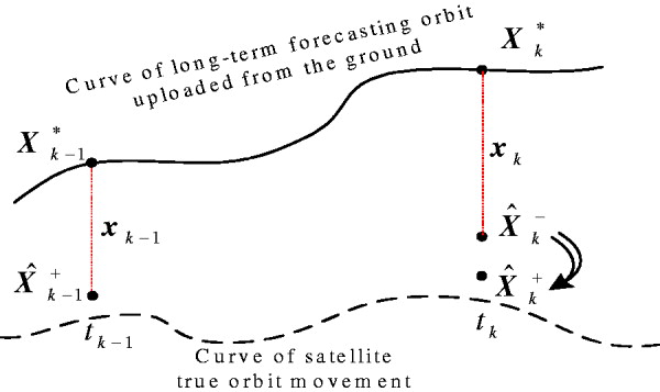
Figure 2. Orbit prediction based on the long term ephemeris uploaded.
2.1.1. Generation of Long-term Ephemeris Prediction Uploaded from the Ground
The long-term ephemeris prediction is achieved by long-term precise orbit prediction of all of the satellites of the navigation constellation. Due to the fact that the calculation is performed on the ground, the best dynamical models for satellites’ orbits can be used to improve the prediction accuracy. In addition, the editing for the precise orbit prediction is also needed to meet the requirements of both the data transmission technology from the ground antenna to satellites and the satellite hardware storage. Therefore, the algorithm used for the long-term ephemeris prediction performed on the ground includes two aspects, the first is the precise prediction of the long-term orbit and the second is the numerical representation of satellite orbits; i.e. editing of the ephemeris. One of the editing methods for the ephemeris prediction is the navigation message, such as the GPS broadcast navigation message. These data are from the ground control segment and becomes input data for the onboard autonomous orbit determination algorithm. In this paper, we conduct an analysis of the accuracy of orbit prediction as follows.
Usually, the main factor that influences the accuracy of long-term orbit prediction is the satellite's dynamic model. In the 1990s, the accuracy of the dynamic model of GPS satellites was about 1×10⁻⁹m/s2 or higher, where the position error in the three-dimensional components by 1-day orbit prediction is within 1 m, by 60-day in the order of 1 km and by 90-day about 1∼10 km. The accuracy of the predictions is equivalent to the User Ranging Error (URE), of 6 m at the end of 10 hours, 200 m at the end of 14 days, and 1500 m (Ananda, Reference Ananda, Bernstein and Cunningham1991) at the end of 180 days.
2.1.2. Selection of State Variable Type for the Autonomous Orbit Determination Algorithm
In spacecraft orbital dynamics, usually, the following four types of state variables are used: the position velocity ![]() , the classical Kepler roots(a,e,i,Ω,ω,M) and the first and second class non-singularity variables. The first and second class non-singularity variables are a combination of classical Kepler roots (Liu, Reference Liu2000). The first class non-singularity variables are
, the classical Kepler roots(a,e,i,Ω,ω,M) and the first and second class non-singularity variables. The first and second class non-singularity variables are a combination of classical Kepler roots (Liu, Reference Liu2000). The first class non-singularity variables are ![]() and they are suitable for satellites with small eccentricity. The second class non-singularity variables are a,
and they are suitable for satellites with small eccentricity. The second class non-singularity variables are a, ![]() h=cos Ω sin i/2,k=sin Ω sin i/2,
h=cos Ω sin i/2,k=sin Ω sin i/2,![]() and they are suitable for satellites with small eccentricity and small inclination. These four types of state variables have different applicability and performance (Wang, Reference Wang2007). For the purpose of generality, the algorithm that should be applicable not only for the MEO/IGSO satellite with small eccentricity but also for the GEO satellites with small eccentricity and small inclination should be used. The algorithm proposed in this paper is based on the second class non-singularity variables (Liu, Reference Liu2000), i.e.,
and they are suitable for satellites with small eccentricity and small inclination. These four types of state variables have different applicability and performance (Wang, Reference Wang2007). For the purpose of generality, the algorithm that should be applicable not only for the MEO/IGSO satellite with small eccentricity but also for the GEO satellites with small eccentricity and small inclination should be used. The algorithm proposed in this paper is based on the second class non-singularity variables (Liu, Reference Liu2000), i.e.,
where a is the orbital semi-major axis, e is the orbital eccentricity, i is the orbital inclination, Ω is the right ascension of ascending node, ![]() , ω is the angular of perigee and M is the mean anomaly.
, ω is the angular of perigee and M is the mean anomaly.
The conversions between different types of state variables can be found in the references (Liu, Reference Liu, Zhang and Liao1999; Hu, Reference Hu, Huang and Liao2000).
2.1.3. An Analytical Solution to the Determination of the Onboard State Transition Matrix
The determination of the state transition matrix and the prediction of the long-term orbit can be performed simultaneously, and the numerical integration method can be used (Tapley, Reference Tapley, Schutz and Born2004; Hu, Reference Hu, Huang and Liao2000). Similarly, due to the constraints on the ground-to-satellite data transmission and the satellite hardware storage, the state transition matrix needs to be simplified.
Generally, the data volume of the state transition matrix is six times as much as that of the orbit state variables. The algorithm proposed in this paper adopts an analytical solution to the determination of the on-board state transition matrix. The formulae and the validity of the solution are described and presented below.
The variables of the state transition matrix also employ the second class non-singularity variables, thus the state transition matrix Φ are composed of two parts as follows (Tapley, Reference Tapley, Schutz and Born2004; Wang, Reference Wang, Liu and Cheng2010):
where Φ(0) is part of two-body motion, Φ(1) is the perturbation part of the Earth flat rate J 2. The formulae for the calculation of these two parts are:


where each element in Φ(1) can be expressed as:
![$$\openup5\left\{ {\matrix{ {b_{21} = - \eta _0 \left[ - \displaystyle{ 7 \over {2a}}\tilde \omega _1 (t - t_0 )\right]} \hfill\cr {b_{22} = - \eta _0 \left[ - \displaystyle{{4\xi _0} \over {1 - e^2}} \tilde \omega _1 (t - t_0 )\right]}\hfill \cr {b_{23} = - \left[1 + \displaystyle{4 \over {1 - e^2}} \eta _0^2 \right]\tilde \omega _1 (t - t_0 )} \hfill\cr {b_{24} = - \eta _0 \left[\left( - \displaystyle{5 \over 2}\right)8h_0 (1 - 2(h_0^2 + k_0^2 )) + 4h_0 \right]\left(\displaystyle{{3J_2} \over {2p^2}} \right)n(t - t_0 )} \cr \displaystyle{b_{25} = - \eta _0 \left[\left( - {5 \over 2}\right)8k_0 (1 - 2(h_0^2 + k_0^2 )) + 4k_0 \right]\left({{3J_2} \over {2p^2}} \right)n(t - t_0 )} \cr}} \right.$$](https://static.cambridge.org/binary/version/id/urn:cambridge.org:id:binary:20151022042007115-0798:S0373463311000397_eqn8.gif?pub-status=live)
![$$\left\{ {\openup5\matrix{ {b_{31} = \xi _0 \displaystyle\left[ - {7 \over {2a}}\tilde \omega _1 (t - t_0 )\right]} \hfill\cr {b_{32} = \displaystyle\left[1 + {4 \over {1 - e^2}} \xi _0^2 \right]\tilde \omega _1 (t - t_0 )} \hfill\cr {b_{33} = \xi _0 \displaystyle\left[ - {{4\eta _0} \over {1 - e^2}} \tilde \omega _1 (t - t_0 )\right]}\hfill \cr {b_{34} = \xi _0 \displaystyle\left[\left( - {5 \over 2}\right)8h_0 (1 - 2(h_0^2 + k_0^2 )) + 4h_0 \right]\left({{3J_2} \over {2p^2}} \right)n(t - t_0 )} \cr {b_{35} = \xi _0 \displaystyle\left[\left( - {5 \over 2}\right)8k_0 (1 - 2(h_0^2 + k_0^2 )) + 4k_0 \right]\left({{3J_2} \over {2p^2}} \right)n(t - t_0 )} \cr}} \right.$$](https://static.cambridge.org/binary/version/id/urn:cambridge.org:id:binary:20151022042007115-0798:S0373463311000397_eqn9.gif?pub-status=live)
![$$\left\{ {\openup5\matrix{ {b_{41} = - k_0 \displaystyle\left[ - {7 \over {2a}}{\rm \Omega}_1 (t - t_0 )\right]}\hfill \cr {b_{42} = - k_0 \displaystyle\left[{{4\xi _0} \over {1 - e^2}} {\rm \Omega}_1 (t - t_0 )\right]} \hfill\cr {b_{43} = - k_0 \displaystyle\left[{{4\eta _0} \over {1 - e^2}} {\rm \Omega} _1 (t - t_0 )\right]}\hfill \cr {b_{44} = - k_0 \displaystyle\left[4h_0 \left({{3J_2} \over {2p^2}} \right)n(t - t_0 )\right]}\hfill \cr {b_{45} = - \displaystyle\left[{\rm \Omega}_1 + 4k_0^2 \left({{3J_2} \over {2p^2}} \right)n\right](t - t_0 )} \cr}} \right.$$](https://static.cambridge.org/binary/version/id/urn:cambridge.org:id:binary:20151022042007115-0798:S0373463311000397_eqn10.gif?pub-status=live)
![$$\left\{ {\openup5\matrix{ {b_{51} = h_0 \displaystyle\left[ - {7 \over {2a}}{\rm \Omega}_1 (t - t_0 )\right]} \hfill\cr {b_{52} = h_0 \displaystyle\left[{{4\xi _0} \over {1 - e^2}} {\rm \Omega}_1 (t - t_0 )\right]}\hfill \cr {b_{53} = h_0 \displaystyle\left[{{4\eta _0} \over {1 - e^2}} {\rm \Omega} _1 (t - t_0 )\right]}\hfill \cr {b_{54} = \displaystyle\left[{\rm \Omega} _1 + 4h_0^2 \left({{3J_2} \over {2p^2}} \right)n\right](t - t_0 )} \cr {b_{55} = h_0 \displaystyle\left[4k_0 \left({{3J_2} \over {2p^2}} \right)n(t - t_0 )\right]} \hfill\cr}} \right.$$](https://static.cambridge.org/binary/version/id/urn:cambridge.org:id:binary:20151022042007115-0798:S0373463311000397_eqn11.gif?pub-status=live)
![$$\openup5\left\{ {\matrix{ {b_{61} = -\displaystyle {7 \over {2a}}\lambda _1 (t - t_0 )} \hfill\cr {b_{62} = \displaystyle{{\xi _0} \over {1 - e^2}} (3M_1 + 4 {\tilde \omega}_1 )(t - t_0 )} \hfill\cr {b_{63} = \displaystyle{{\eta _0} \over {1 - e^2}} (3M_1 + 4{\tilde \omega}_1 )(t - t_0 )} \hfill\cr {b_{64} = \displaystyle\left[\left( - {3 \over 2}\sqrt {1 - e^2} - {5 \over 2}\right)8h_0 (1 - 2(h_0^2 + k_0^2 )) + 4h_0 \right]\left({{3J_2} \over {2p^2}} \right)n(t - t_0 )} \cr {b_{65} = \displaystyle\left[\left( - {3 \over 2}\sqrt {1 - e^2} - {5 \over 2}\right)8k_0 (1 - 2(h_0^2 + k_0^2 )) + 4k_0 \right]\left({{3J_2} \over {2p^2}} \right)n(t - t_0 )} \cr}} \right.$$](https://static.cambridge.org/binary/version/id/urn:cambridge.org:id:binary:20151022042007115-0798:S0373463311000397_eqn12.gif?pub-status=live)

In the above formulae, a,e,i,p=a(1−e 2) and n=a −3/2 are the instantaneous orbital elements at epoch time t 0 (they can also be named a 0, e 0, i 0, …); ![]() , e 0 and i 0 appeared in M 1,ω 1 and Ω1 (equation (13)) can be obtained by:
, e 0 and i 0 appeared in M 1,ω 1 and Ω1 (equation (13)) can be obtained by:
where ![]() ,
, ![]() .
.
In this analytical solution, only the items of the central gravitational and the oblateness rate perturbation of the Earth are considered. The remaining higher order perturbation items (δΦ), such as the higher order non-spherical gravitational perturbation of the Earth, the third-body perturbation of moon and sun etc., are ignored. Table 1 lists the perturbation magnitude of MEO/IGSO/GEO satellites, for the solar radiation pressure perturbation, a typical value of 109, which is equivalent to 10 m2/1000 kg, for the effective surface-mass ratio of the satellites is used. It should be noted that the magnitude values in this table are in fact the results of their actual values divided by the central gravity of the Earth.
Table 1. Magnitudes of perturbations of MEO/GEO/IGSO satellites.

From Table 1, it can be seen that, for all the three satellite systems, the higher order perturbations ignored in equation (5) are mainly the solar and lunar gravitational perturbation terms, the maximum magnitude of which is 2×10⁻⁵. Given that the order of the long-term orbit prediction error (i.e. x in equation (2)) is less than 10 km (10−3 under the dimensionless unit of the Earth), based on equations (2) and (5), the order of the one-step orbit prediction error can be estimated as:
Here, the step-size is 15 minutes. In the International System of Units, the order of δ xk in equation (16) is 0·13 m, which means the one-step prediction error of orbit is 0·13 m.
Due to the fact that the inter-satellite ranging accuracy is 1 m, which is larger than the one-step prediction error, the proposed analytical solution to the calculation of the onboard state transition matrix matches to the accuracy of inter-satellite ranging. In addition, compared to the state transition matrix uploaded from the ground, costs in ground-to-satellite data transmission and data storage units of satellite hardware, which are very high for space missions, can be saved. Therefore, the proposed solution to the determination of the state transition matrix has advantages.
2.2. Kalman Filter for Onboard Autonomous Orbit Determination
As a recursive algorithm, the Kalman filter can be used for calculation of on-board autonomous orbit determination in real-time. In this paper, the extended Kalman filter (EKF) is used to estimate the orbit state variables. The main procedure is as below (Tapley, Reference Tapley, Schutz and Born2004; Lin, Reference Lin, Qin and Chu2010).
2.2.1. Kalman Gain Calculation
where subscript k denotes k-th epoch, Rk is the covariance matrix of inter-satellite ranging at epoch t k, Pk− is the state variable covariance matrix at t k, which is the covariance of one-step prediction error, calculated as follows:
where Φ(t k−1,t k) is the state transition matrix of orbital variables, and Qk is the dynamic noise covariance matrix at t k.
In equation (17), Hk is the measurement matrix calculated by
where the subscripts m, and n denote the two satellites associated with the inter-satellite two-way ranging, the onboard distributed autonomous orbit determination algorithm is performed in both satellites, equation (19) is the measurement matrix for satellite m; ![]() is the approximate value of the distance between satellites m and n at t k; rm and rn are the position vectors of the satellites m and n at t k respectively;
is the approximate value of the distance between satellites m and n at t k; rm and rn are the position vectors of the satellites m and n at t k respectively; ![]() and
and ![]() are the predicted orbit state variables of satellites m and n at t k, respectively, which can be calculated using equations (3) and (4). The two matrices at the right-hand side of equation (19) are for the measurement geometry and orbit geometry respectively, and they can be calculated by (Wang, Reference Wang2007; Liu, Reference Liu, Zhang and Liao1999):
are the predicted orbit state variables of satellites m and n at t k, respectively, which can be calculated using equations (3) and (4). The two matrices at the right-hand side of equation (19) are for the measurement geometry and orbit geometry respectively, and they can be calculated by (Wang, Reference Wang2007; Liu, Reference Liu, Zhang and Liao1999):
The expressions for the six elements in equation (21) are as follows:

where r=(x,y,z)Tis the position vector of the satellite; ![]() is the velocity vector of the satellite and:
is the velocity vector of the satellite and:
![$$\left\{\hskip-3 {\openup5\matrix{ {A = \displaystyle{a \over p}\left[ - (\cos u + \xi ) - \displaystyle\left({r \over p}\right)(\sin u + \eta )(\xi \sin u - \eta \cos u)\right]} \cr {B = \displaystyle{{ar} \over {\sqrt p}} \left[\sin u + \left({a \over r}\right){{\sqrt {1 - e^2}} \over {1 + \sqrt {1 - e^2}}} \eta + \left({r \over p}\right)(\sin u + \eta )\right]} \hfill\cr {C = - \displaystyle{a \over p}\left[(\sin u + \eta ) - \left({r \over p}\right)(\cos u + \xi )(\xi \sin u - \eta \cos u)\right]} \cr {D = - \displaystyle{{ar} \over {\sqrt p}} \left[\cos u + \left({a \over r}\right){{\sqrt {1 - e^2}} \over {1 + \sqrt {1 - e^2}}} \xi + \left({r \over p}\right)(\cos u + \xi )\right]} \hfill\cr}} \right.$$](https://static.cambridge.org/binary/version/id/urn:cambridge.org:id:binary:20151022042007115-0798:S0373463311000397_eqn23.gif?pub-status=live)


where a, ξ, η, h, k, λ are the second class non-singularity variables defined in equation (4); p=a(1−e 2); ![]() is the distance between the satellite and the centre of the Earth;
is the distance between the satellite and the centre of the Earth; ![]() is the latitude angle of the satellite, f is the true anomaly of the satellite orbit and
is the latitude angle of the satellite, f is the true anomaly of the satellite orbit and ![]() ; ω is the angular of the perigee; and Ω is the right ascension of the ascending node.
; ω is the angular of the perigee; and Ω is the right ascension of the ascending node.
2.2.2. The Measurement Update
where ρ mn and ρ mn−(Xk−) are the measured and predicted distances between the two satellites at t k respectively. The predicted distance is calculated from the predicted orbit state variables at t k.
2.3. Pre-processing of Two-way Inter-satellite Pseudo Ranging
The pseudo-range is obtained in the same way as GPS pseudo-range with pseudo random code, so the clock parameters of one pair of satellites are considered. The original inter-satellite ranging measurements based on the inter-satellite crosslink are the emission time and the reception time of the signal. Given the problem with the asynchronous clocks of the constellation satellites, it is necessary to use two-way pseudo-range measurements. Dual-frequency measurement is necessary to correct the ionospheric delay. For a pair of satellites that establish an inter-satellite crosslink, each satellite collects four pseudo-range measurements; i.e. two pseudo-range measurements from the emission process and the other two inform the receiving process. Several corrections such as the phase centre offset correction, relativistic effect correction and ionospheric delay correction for these measurements need to be carried out in order to obtain more precise pseudo-range between the mass centres of the two satellites. The clock information and ephemeris information are coupled in one-way ranging, and they can be decoupled from a pair of two-way ranging measurements. The difference of the range-pair removes geometric information and their sum removes the clock information. The corrected pseudo ranges are decoupled into two independent parts: derived clock measurements and ephemeris measurements. The procedure of the decoupling is as follows (Ananda, Reference Ananda, Bernstein and Cunningham1991).
First, assuming that satellite m transmits a signal and satellite n receives the signal, then the measured pseudo-range from satellite m to satellite n, i.e., PR nm, can be written as:
where D nm is the geometric distance from satellite m at the signal's transmitting moment to satellite n at the receiving moment, ΔD ion is the ionospheric delay correction, ![]() and
and ![]() are clock errors of satellites m and n respectively, and c is the speed of light in vacuum.
are clock errors of satellites m and n respectively, and c is the speed of light in vacuum.
Secondly, similar to the above equation, for the measured pseudo-range from satellite n to satellite m:
In fact, equations (29) and (30) are the observation equations of the two-way pseudo-ranging.
After the ionospheric delays are corrected from the two-way pseudo ranging observations, the corrected pseudo-ranges can be transformed into the ones that have same emission and reception time. Let D be the geometric distance of the two satellites at this moment, then:
Let the average value of the two-way pseudo-ranges be Z d, then it can be used for ρ mn in equation (27).
In addition, the time period (or the session) during which the two-way pseudo ranging measurements of the pair of satellites are continuously collected is short, e.g., generally shorter than 15 minutes, the satellite clock drift during such a period will not change much. In this case, the satellite clock drift could be treated as a constant in the session.
2.4. Analysis of Calculation and Storage Needed for the Proposed Algorithm
The two main aspects determining the applicability of an algorithm/approach for on-board autonomous orbit determination are the amount of computation and storage needed. Test results of the algorithm proposed in this paper using Windows platform are as follows:
• the data processing of each ranging frame needed 5·8 M times floating-point operations;
• when the session length was set to 15 minutes, the calculation of the algorithm needed an average of 0·0065 MHz, which is significantly smaller compared to the centralised scheme which needed an average computation of 0·155 MHz;
• in the aspect of storage, the on-board algorithm software occupied less than 50 K bytes of storage space. The calculation process demanded for 45 K bytes storage space, 40 K bytes of which are needed by the long-term ephemeris prediction uploaded from the ground. When the algorithm based on an on-board numerical integrator for orbit determination was used, the amount of calculation significantly increased.
The test results suggest that the distributed algorithm for autonomous orbit determination based on the long-term ephemeris prediction uploaded from the ground is applicable for space missions in terms of its less calculation amount and less storage needed.
3. SIMULATION OF THE ONBOARD AUTONOMOUS ORBIT DETERMINATION ALGORITHM
Simulation for the onboard autonomous orbit determination algorithm consists of five modules that are for the following five purposes respectively:
Module 1: the generation of standard orbits for navigation satellites,
Module 2: the inter-satellite crosslink ranging,
Module 3: the algorithm for onboard autonomous orbit determination,
Module 4: the generation of the long-term ephemeris prediction uploaded from the ground,
Module 5: the evaluation of performance.
The diagram of the modules is shown in Figure 3.

Figure 3. The diagram for the simulation of the on-board autonomous orbit determination algorithm.
Module 1, i.e. the one for the generation of standard orbits for all the constellation satellites, is used to generate data of orbital motion in the real space. This data is the input of module 2 for the generation of inter-satellite distances. The data from module 1 is also used as the standard orbit and used for the assessment of the accuracy of the autonomous orbit determination algorithm. Module 2 generates two-way simulated pseudo-range measurement values and it is based on both the topology configuration of the inter-satellite crosslink and the visibility of the satellites. The dynamics model used in module 3 is different from that of module 1.
The settings for the dynamics model used in module 1 are:
• Earth gravity field model: WGS84, with the order of 10×10;
• Lunar and solar gravitational perturbations: DE200 numerical planetary ephemeris;
• Earth tidal perturbation;
• Solar radiation pressure perturbation: sunlight pressure model uses the CODE (Springer, Reference Springer, Beutler and Rothacher1999);
• Relativistic effects.
For the dynamics model used in module 4, all the settings are the same as that for module 1 except the following two items:
• Earth gravity field model: WGS84, with the order of 4×4;
• Solar radiation pressure perturbation: sunlight pressure model using CODE and the model parameters have a random error of 2×10⁻⁹m/s2 and a systematic relative error with a value selected from 2%, 5%, 10% and 20%.
3.1. Errors of Long-term Ephemeris Predictions Resulting from Errors of Dynamics Models
Different error values in the dynamics models used in module 4) result in different magnitudes of errors in the generated long-term orbits. We carried out an assessment of the errors of long-term orbit predictions resulting from the five different error settings of the dynamics model specified in the previous section. The URE is calculated as follows:
Where ΔR is radial orbit error, ΔT is tangent orbit error, and ΔN is normal orbit error.
Evaluation results are shown in Figure 4. It should be noted that the URE in Figure 4 stands for the average error of all the satellites in the constellation. Figure 4 shows that the URE values of the long-term ephemeris predictions are approximately linearly amplified with the errors of the dynamical model and these URE values also present small-scale cyclic variations. Figure 5 is the diagram for the evolution of the URE values of the long-term orbit predictions of all the 24 satellites and No.1 satellite respectively in the condition that the 20% systematic error is selected for the solar radiation parameter. Figure 5 indicates that all the 24 satellites have the same trend of error evolution.

Figure 4. UREs of long term orbit predictions from the ground.

Figure 5. URE of long term orbit prediction based on the systematic error of solar radiation model=20%.
From Figure 4, it can be seen that when the systematic error is set to 20% for the solar radiation parameter, the URE value can reach 400 m and 2400 m at the end of 30-day and 180-day predictions, respectively; when 10% is set for the systematic error, these URE values reach 200 m and 1200 m, respectively. Therefore, it is more realistic to use values in the range of 10%−20% for the systematic error of the solar radiation parameter if compared with the accuracy level of the long-term navigation message of GPS in early 1990s: the URE of 1500 m in 180 days (Ananda, Reference Ananda, Bernstein and Cunningham1991).
3.2. Topology Configurations of Inter-satellite Crosslink Ranging
In this paper we considered the four topology configurations for inter-satellite crosslink ranging shown in Table 2. The wide wave beam antenna is such an antenna like UHF crosslink antenna on GPS block IIR satellites, with which the IIR satellite could perform inter-satellite ranging to other in-view satellites. Both the inside and outside flare angles of the wide wave beam inter-satellite crosslink ranging are measured by the centre line of the connection between the satellite and the Earth centre. For the MEO satellite whose orbit altitude is 24 000 km the selection of 15 degrees for the inside flare angle can guarantee the wave beam of inter-satellite crosslink ranging is at higher than 1000 km above the Earth's surface. The three fixed inter-satellite crosslinks are connected as follows: one crosslink is established from the same orbital plane and the other two are from different orbital planes.
Table 2. The four types of topology configurations.
3.3. Simulation and Analysis Results of the Onboard Autonomous Orbit Determination Algorithm
In the simulation, a random white noise, which has zero mean value with 1·0 m2 variance, was used for the generation of inter-satellite ranging measurements. The ranging session was set to15 minutes.
First, we performed a simulation of autonomous orbit determination for Topology 1 for the purpose of checking the correctness and precision of the autonomous orbit determination result. The test result is shown in Figure 6. The five curves in this figure from the bottom to the top are for the cases of 2×10⁻⁹m/s2 random error of the solar radiation model, 2%, 5%, 10% and 20% systematic errors of the solar radiation model parameter, respectively. As we can see, the algorithm is convergent and the URE of the long-term autonomous orbit determination is less than 3·0 m when the systematic error of the solar radiation model parameter is set to 20%.

Figure 6. UREs of autonomous orbit determination of wide wave beam crosslink measurements (Topology type 1).
In March 2001, the United States downloaded the inter-satellite ranging data of six GPS Block IIR satellites to the ground control segment for post-processing for the calculation of the UREs of satellite autonomous navigation. Figure 7 shows the result from reference (Rajan, Reference Rajan2002). From this figure one can see that, on most occasions, the URE values are less than 3 m during the period of 75 days (Rajan, Reference Rajan2002).

Figure 7. Post Processed On-Orbit Performance (Rajan, Reference Rajan2002).
Comparing Figure 6 to Figure 7, we can see that the accuracy of the algorithm proposed in this paper is comparable to that of the ground based, post-processed GPS Block IIR satellite autonomous navigation. Considering the result of Figure 7 was from really GPS IIR satellites' inter-satellite ranging data, more research work on detailed performance of the algorithm is needed in the future.
We also compared the results of autonomous orbit determination of all the four topology type configurations defined in Table 2, as showed in Figure 8. It is noted that the UREs in Figure 8 are the mean value of the session period of autonomous orbit determination. It can be seen that topology type 1 performs the best, followed by topology type 4, and the rest two topology types’ UREs are both greater than 3·0 m. These results can provide a reference to the topology configuration design of inter-satellite crosslink ranging.

Figure 8. UREs using crosslink measurements of 4 topology types.
In addition, we also simulated and analyzed the UREs of the autonomous orbit determination algorithm using inter-satellite ranging measurements containing both random and periodical systematic error. The selections of the errors of the inter-satellite ranging measurements are:
• The random error: mean value 0·0 m and the variance 1·0 m2;
• The systematic error: the value of the constant term is 0 m and the period term is equal to one orbital period. The three selections of the amplitude of the periodic systematic error are 0·3 m, 0·9 m and 1·5 m.
The ranging session was still set to 15 minutes. It should be noted that the topology configuration of inter-satellite crosslink ranging, as mentioned before, consists of four fixed crosslinks and two of the links are in the same orbital plane and the other two links are in different orbital planes. The simulation results are displayed in Figure 9 which shows the UREs of autonomous orbit determination using inter-satellite ranging measurements with the amplitudes of the systematic error equal to 0·0 m, 0·3 m, 0·9 m or 1·5 m, respectively and the period equal to the orbital period. The case of amplitude equal to 0·0 m means no systematic error in inter-satellite ranging. Figure 9 suggests that the autonomous orbit determination algorithm can also deal with inter-satellite ranging measurements contaminated by periodical systematic errors and the URE of orbit determination is the same regardless of whether the measurement contains the systematic error.

Figure 9. UREs of autonomous orbit determination using measurements containing different periodic system errors.
4. CONCLUSIONS
In this paper, a distributed algorithm for onboard autonomous orbit determination based on the long-term ephemeris prediction uploaded from the ground is proposed. The onboard autonomous orbit prediction and filtering correction of the measurements are discussed in detail. The simulation results show that the autonomous orbit determination algorithm is effective, especially under the wide beam topology configuration type 1 of inter-satellite crosslink ranging. The proposed algorithm is convergent, its performance is stable and the URE value of the long-term autonomous orbit determination is less than 3·0 m. Tests of the software indicates that, compared to both approaches of using a on-board numerical orbit integrator and centralised data processing, the proposed algorithm has the advantages of fewer calculations and less storage needed. That implies the significance and suitability of the proposed algorithm for space missions. In addition, the analytical solution to the on-board state transition matrix proposed in this paper can save a great amount of resources for both satellite-ground data transmission and on-board data storage. All these imply that the proposed method for onboard autonomous orbit determination has great practical prospects for space missions.


