


1. INTRODUCTION
The growing reliance on Global Navigation Satellite System (GNSS) radio signals for precise positioning, navigation and timing applications of space and ground-based technological infrastructure requires robust algorithms for the mitigation of ionospheric scintillation effects. The amplitude and phase of trans-ionospheric GNSS signals encounter random fluctuations due to ionospheric irregularities, which cause radio signal diffraction (Crane, Reference Crane1977). The deep/high amplitude fade rates cause data loss due to the drop of signal-to-noise ratio values below a GNSS receiver's tracking threshold. Ionospheric scintillation effects threaten the accuracy and integrity of GNSS services due to the fading of Signals In Space (SIS) (Weng et al., Reference Weng, Ji, Chen and Liu2014; Forte, Reference Forte2012; Aquino et al., Reference Aquino, Moore, Dodson, Waugh, Souter and Rodrigues2005).
Ionospheric scintillations exhibit large day-to-day variations depending on the receiver's geographical location (latitude, longitude), local time, season, solar and geomagnetic activity (Aarons, Reference Aarons1982). Moreover, the received GNSS scintillation signal is a non-stationary signal because of the slowly varying background ionosphere (Aquino et al., Reference Aquino, Moore, Dodson, Waugh, Souter and Rodrigues2005).
Conventional time-invariant digital filters such as the Butterworth filter used in current GNSS receivers during detrending cannot accurately filter non-stationary components of scintillated GNSS signals at different frequencies (Mushini et al., Reference Mushini, Jayachandran, Langley, MacDougall and Pokhotelov2012). Therefore, predicting and mitigating the impact of ionospheric scintillations on GNSS receivers requires advanced and robust GNSS signal processing algorithms for modelling, decomposition and detection of singularities and removal of noisy components. Mushini et al. (Reference Mushini, Jayachandran, Langley, MacDougall and Pokhotelov2012) and Ruan et al. (Reference Ruan, Zhang, Luo and Long2017) proposed wavelet filtering for properly preserving the local time-frequency information and removing non-stationary signals of raw GNSS signals at different time-scales. Nevertheless, a priori selection of a mother wavelet influences the performance of wavelet filtering. Empirical Mode Decomposition (EMD) based on Neyman Pearson's detector was implemented for the detection and mitigation of ionospheric scintillation effects (Ratnam et al., Reference Ratnam, Sivavaraprasad and Lee2015). However, the shortcomings of EMD are a lack of strong mathematical theory, mode-mixing problems, the problem of its stopping criterion in deriving the Intrinsic Mode Functions (IMFs) and its sensitivity to noise and sampling, which limit its implementation as a robust algorithm for mitigating scintillation effects. Complementary Ensemble EMD (CEEMD) in combination with Multifractal Detrended Fluctuation Analysis (MF-DFA) was implemented for mitigating the scintillation noise due to ionospheric irregularities in GNSS signals (Miriyala et al., Reference Miriyala, Koppireddi and Chanamallu2015). Nevertheless, CEEMD is a noise-assisted recursive decomposition method, which means it is not fully intrinsic and data-driven (Herrera et al., Reference Herrera, Han and Van der Baan2014).
In this paper, Time-Frequency Representation (TFR) of trans-ionospheric GNSS signal scintillations has been investigated using a Synchrosqueezing Transform (SST) (Daubechies et al., Reference Daubechies, Lu and Wu2011). This is useful in examining local features of complex structures of GNSS signals in both time and frequency domains. SST is an adaptive and informative TFR technique, applied for seismic and micro-seismic data for successful noise reduction (Daubechies et al., Reference Daubechies, Lu and Wu2011, Herrera et al., Reference Herrera, Han and Van der Baan2014, Mousavi et al., Reference Mousavi, Langston and Horton2016, Thakur et al., Reference Thakur, Brevdo, Fučkar and Wu2013). The multi-components of GNSS signals have been extracted for the detection and mitigation of ionospheric scintillation noise using the DFA algorithm (Peng et al., Reference Peng, Buldyrev, Havlin, Simons, Stanley and Goldberger1994). In Section 2, the theory of the SST-DFA algorithm is described, and experimental results and discussion are given in Section 3. Conclusions are outlined in Section 4.
2. THEORY - SYNCHROSQUEEZING TRANSFORM AND DETRENDED FLUCTUATION ANALYSIS (SST-DFA) FOR MULTICOMPONENT ANALYSIS AND MITIGATION OF IONOSPHERIC SCINTILLATIONS EFFECTS
The SST is an adaptive wavelet-based time-frequency decomposition tool for non-linear and non-stationary signals. It is a special reassignment technique and an alternative method of EMD (Daubechies et al., Reference Daubechies, Lu and Wu2011). It provides high frequency resolution and time localisation of a given GNSS signal and sharpens time-frequency analysis by reassigning the values of time-frequency characteristics based on their local oscillations. The invertible SST transform recovers the instantaneous amplitude and frequencies and breaks down the signal into a number of IMFs with time-varying oscillatory characteristics (Thakur et al., Reference Thakur, Brevdo, Fučkar and Wu2013). The general form of GNSS affected by ionospheric scintillations with amplitude fades and phase variations is given by Fu et al. (Reference Fu, Han, Rizos, Knight and Finn1999) and Ratnam et al. (Reference Ratnam, Sivavaraprasad and Lee2015) as:
 $${S}_{n}({t})=(\hbox{A} \ast \partial {A})_{\rm n}(\hbox{t})\hbox{e}^{{\rm i}\pi ({\Oslash}+\partial \hbox{\o})_{\rm n}(\hbox{t})}$$
 where S(t) is a multi-component GNSS signal, n is the number of IMFs,  $\hbox{n}=1\comma \; 2\comma \; 3\comma \; \ldots \hbox{N}\comma \; \hbox{A}\comma \; \hbox{\o}$ are the amplitude and phase of the GNSS signal, ∂ A,
  $\partial \hbox{\o}$ are the amplitude fades and phase variations, respectively due to ionospheric scintillations, e(t) is the scintillation noise and S n(t) is the n number of oscillatory IMFs of SST with time varying amplitude and frequency.
The implementation algorithm of SST-DFA in the retrieval of IMFs and mitigation of scintillation noise is given by:
Step 1: Calculate the Continuous Wavelet Transform (CWT) of GNSS scintillated signal S(t):
 $$W_S(a,b) = \displaystyle{1 \over {\sqrt a }}\int S (t)\Psi ^*\left( {\displaystyle{{t-b} \over a}} \right)dt$$
where, a represents a scaling parameter (a > 0) and b represents a translating factor of CWT coefficients, respectively. Ψ(t) is the mother wavelet (Morlet is chosen as justified and defined below in Step 2) and Ψ*(t) is the complex conjugate of the mother wavelet chosen, that is, Ψ(t). The translation parameter, b, shifts Ψ(t) in time and the temporal width of Ψ(t) is controlled by the scaling parameter, a.
Step 2: Collate selective parameters such as mother wavelet type and wavelet threshold γ (Herrera et al., Reference Herrera, Han and Van der Baan2014).
In this paper, a hard wavelet threshold γ, γ > 0 has been chosen, which discards the lowest CWT magnitude, | Wf | ≤ γ, at which ω is deemed trustworthy. Its value determines the level of filtering (Thakur et al., Reference Thakur, Brevdo, Fučkar and Wu2013). γ = 10−7 is used in the numerical implementation.
The Morlet mother wavelet is used in this paper. The Morlet wavelet, as per Torrence and Compo (Reference Torrence and Compo1998), is defined as:
 $$\psi _0(t) = \displaystyle{{e^{i\omega _0t}} \over {\root 4 \of {\pi e^{t^2/2}} }}$$
where t refers to dimensionless time and ω 0 refers to dimensionless frequency; ω represents angular frequency (Mallat, Reference Mallat1999); the Morlet with parameter ω0 = 6 provides good stability in time and frequency localisation and better characteristic extraction of GNSS scintillation signals with appreciable resolution (Ahmed et al., Reference Ahmed, Tiwari, Strangeways, Dlay and Johnsen2015, Domingues et al., Reference Domingues, Mendes and Da Costa2005; Torrence and Compo, Reference Torrence and Compo1998). The Morlet wavelet is considered for GNSS scintillation signal processing as it provides good time and frequency resolution/localisation due to its small time-bandwidth product and its non-orthogonality (Torrence and Compo Reference Torrence and Compo1998; Mallat, Reference Mallat1999; Materassi and Mitchell, Reference Materassi and Mitchell2007; Mushini et al., Reference Mushini, Jayachandran, Langley, MacDougall and Pokhotelov2012; Wang et al., Reference Wang, Morton, Zhou, van Graas and Pelgrum2012; Najmafshar et al., Reference Najmafshar, Skone and Ghafoori2014). Moreover, the Morlet mother wavelet exactly reproduces the sudden fades in GNSS scintillated signals due to ionospheric complex plasma dynamics and irregularities (Materassi and Mitchell, Reference Materassi and Mitchell2007; Mushini et al., Reference Mushini, Jayachandran, Langley, MacDougall and Pokhotelov2012).
Step 3: Calculate W S(a, b) for the instantaneous time-frequency information of S(t).
Step 4: Calculate the synchrosqueezing function.
This is based on the reassignment of time-scale plane to Time-Frequency (T-F) plane, that is, function ((a; b) to (W S(a, b); b)) (Herrera et al., Reference Herrera, Han and Van der Baan2014, Mousavi et al., Reference Mousavi, Langston and Horton2016, Thakur et al., Reference Thakur, Brevdo, Fučkar and Wu2013). It is given by:
 $$T_S(w_l,b) = \displaystyle{1 \over {\Delta w}}\sum\limits_{a_n: \vert w(a_n,b)-w \vert \le {\textstyle{{\Delta w} \over 2}}} {W_S(a_n,b)a^{-{\textstyle{3 \over 2}}}\Delta a_n} $$
where T S(wl, b) is the synchrosqueezed TFR of the GNSS scintillated signal given by reallocating the coefficients of CWT. Then, the instantaneous frequencies are extracted from T S(wl, b) (Wu et al., Reference Wu, Flandrin and Daubechies2011). Δw = wl − wl−1 is the frequency range where w l is the centre frequency.
Step 5: Extract the individual IMFs of multi-component GNSS signal.
IMFs are retrieved from the discrete synchrosqueezed inversion CWT using the formula provided by (Herrera et al., Reference Herrera, Han and Van der Baan2014, Thakur et al., Reference Thakur, Brevdo, Fučkar and Wu2013):
 $$S_n(t_m) = 2C_{\hbox{\o}}^{-1} Re\left( {\sum\limits_{l\in L_n(t_m)} {{\tilde{T}}_{\tilde{S}}(\hbox{w}_l,t_m)} } \right)$$
 where  $\widetilde{T}_{\tilde{S}}$ is the discrete synchrosqueezed transform,
  $C_{\hbox{\o}}^{-1}$ is the dependent constant of chosen wavelet, t m(t 0 + mΔt) is discrete time at a sampling rate of Δ t, S n(t m) is the retrieved n-th IMF, m = 1, 2, 3, …, n − 1 and l is the small frequency band.12 IMFs have been chosen in this paper.
Step 6: Reconstruct the GNSS scintillated signal from IMFs.
Step 7: Apply DFA to identify the ionospheric scintillation effects on GNSS signals.
The SST IMFs with scintillation noise have to be detected and mitigated to recover the scintillation-free GNSS signal. The separation of SST-IMFs with scintillation noise depends on the DFA scaling exponent or threshold α - if α ≤ 0.5 (anti-correlated and contains white noise) and 0.5 ≤ α (correlated noise-free time series) (Liu et al., Reference Liu, Yang, Li and Yin2016; Peng et al., Reference Peng, Buldyrev, Havlin, Simons, Stanley and Goldberger1994; Sivavaraprasad et al., Reference Sivavaraprasad, Padmaja and Ratnam2017).
Thus, the binary hypothesis decision criterion of the DFA method to classify the received GNSS signal propagated through ionosphere is given by:
DFA(SST − IMF) > α, null hypothesis (scintillation-free IMF).
DFA(SST − IMF) < α, alternate hypothesis (IMF with scintillation noise).
where α describes the degree of correlation in the time series or IMF.
Step 8: Separate the GNSS scintillated signal components using the DFA algorithm.
To remove noise from the GNSS-scintillated signal, each SST-IMF is processed through the DFA algorithm (Liu et al., Reference Liu, Yang, Li and Yin2016; Peng et al., Reference Peng, Buldyrev, Havlin, Simons, Stanley and Goldberger1994; Sivavaraprasad et al., Reference Sivavaraprasad, Padmaja and Ratnam2017).
3. RESULTS AND DISCUSSION
3.1. Application of SST-DFA for CSM simulated scintillation data
In order to test the performance of the SST algorithm, amplitude scintillation data under catastrophic ionospheric scintillation conditions were simulated from the Cornell Scintillation Model (CSM), which is available at http://gps.ece.cornell.edu/tools.php. The In-phase (I) and Quadra-phase (Q) components were retrieved from the CSM simulator to obtain the amplitude scintillation observations. The samples of CSM amplitude scintillations data describe the rate of signal fading (Figure 1). The CSM data was recorded at a lower Signal to Noise Ratio (C/N 0) for 35 dB-Hz, maximum S4 index (S4 = 0.9) and the lower decorrelation time was 0.1 s. The amplitude scintillation data was sampled at 100 Hz for a period of 60 s and is shown in Figure 1. During the catastrophic scintillation condition, the deep fades of amplitude scintillations were noticed to be as low as −17.5 dB, as seen in Figure 1.

Figure 1. Synthetic (CSM) Amplitude Scintillations Data.
Figure 2 shows the SST time-frequency representation of amplitude scintillations (Equation (3)) to localise both noisy and signal components of interest for better discrimination. The TFR result obtained by the SST (Figure 2) uses a Morlet wavelet and 32 voices per octave. The colour bar represents the low and high-power levels located in the time-frequency map of amplitude scintillations data. The SST highlights the instantaneous amplitude of deep fades at lower and high frequency components in the synchrosqueezed time-frequency plane.
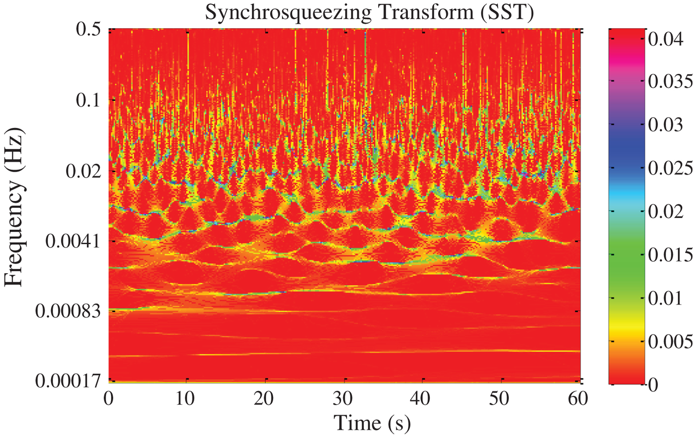
Figure 2. Time-frequency Representation of CSM Amplitude Scintillations Using SST Technique.
The scintillated amplitude signal was decomposed by SST to obtain individual dominant modes or IMFs (Equation (4)), as shown in Figure 3. The 12 SST-IMFs of amplitude scintillation data are shown in panels 1–12 of Figure 3. The SST-IMFs were mapped with respect to their instantaneous (independent) order of frequencies. The highest oscillating components represent the noisy information while the lower frequency ones refer to the required signal component (Miriyala et al., Reference Miriyala, Koppireddi and Chanamallu2015; Mushini et al., Reference Mushini, Jayachandran, Langley, MacDougall and Pokhotelov2012). Clearly, SST-IMFs showed the low and high-frequency oscillations of the given CSM amplitude scintillated signal (Figure 3) with good resolution by providing the instantaneous amplitudes of each frequency component for a given time due to its strong mathematical and reassignment scheme (Herrera et al., Reference Herrera, Han and Van der Baan2014; Mousavi et al., Reference Mousavi, Langston and Horton2016). IMF 1, IMF 4, IMF 5 and IMF 9–11 represent low frequency variations, whereas IMF 2–3, IMF 6–8 and IMF 12 represent the high frequency oscillations (Figure 3).
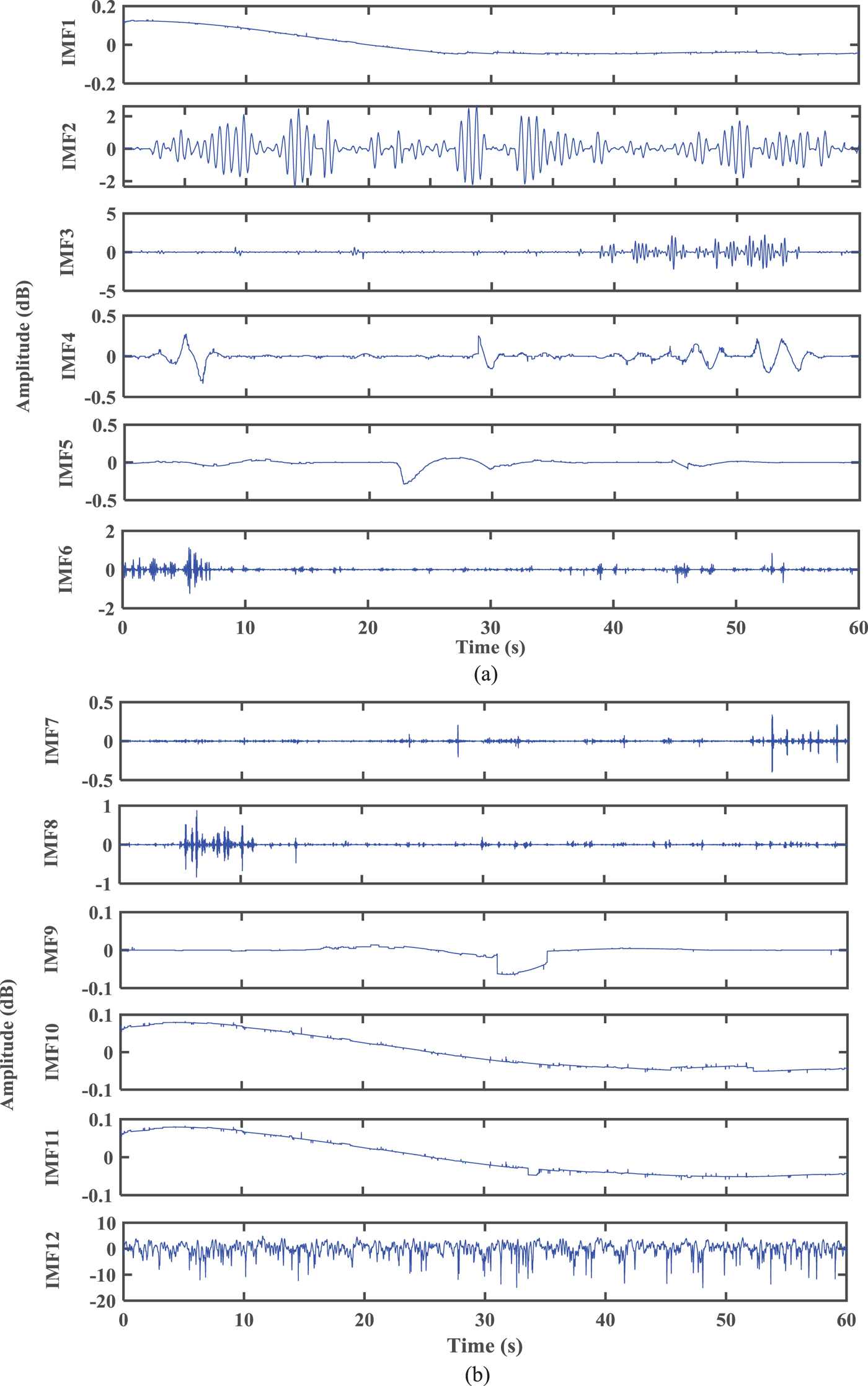
Figure 3. (a) Retrieval of 1-6 multi-components (IMFs) and (b) Retrieval of 7-12 multi-components (IMFs) from CSM synthetic amplitude scintillation data using SST algorithm.
The reconstruction of signal amplitude scintillations using SST IMFs (red dot lines) is shown in Figure 4(a). The reconstruction error for the SST algorithm shown in Figure 4(b) is in the order of 10−16 dB. This indicates that the SST technique is an accurate reconstruction method for retrieving the complete GNSS scintillation signal. For detection and mitigation of scintillation-induced noise in a GNSS signal, DFA was chosen as a detrending tool (Liu et al., Reference Liu, Yang, Li and Yin2016; Sivavaraprasad et al., Reference Sivavaraprasad, Padmaja and Ratnam2017). DFA determines the scaling properties and detects the long-range (persistence) correlations of non-stationary data. It computes the fluctuation of average Root Mean Square (RMS) around the local trend as a function of time scale of time series.

Figure 4. (a) The SST reconstructed amplitude signal and (b) SST reconstruction errors (reconstruction error is approximately zero in the order of 10−16).
The degree of correlation in IMFs was calculated using the DFA scaling exponent, alpha (α). If α is more than 0.5, it indicates that smooth and long-range correlations existed in the IMFs; if not, it is concluded that the IMFs are exhibiting short-range correlations (anti-persistence) due to scintillation noise, which must be neglected (Liu et al., Reference Liu, Yang, Li and Yin2016; Miriyala et al., Reference Miriyala, Koppireddi and Chanamallu2015). The low and high frequency details from IMFs obtained from the SST method were able to delineate the scintillation noisy features that were to be processed through DFA for detection and elimination. Figure 5 shows the DFA alpha values calculated for each SST-IMFs. It may be observed that IMFs 1, 4, 5, 9, 10 and 11 signals were smoother, indicating required signal components and eliminating the remaining IMFs for reconstruction or retrieval of filtered scintillation-free amplitude scintillated GNSS signals (Figure 5). The original CSM amplitude scintillated signal (blue line) versus retrieved scintillation-free amplitude signal using SST-DFA (red line) is shown in Figure 6(a). It may be observed that scintillation noise of 15–16 dB was removed using SST-DFA. Figure 6(b) shows the required SST-DFA filtered scintillation-free signal (red line). The SST-DFA mitigated scintillation noise is shown in Figure 6(c) (brown line).

Figure 5. DFA Threshold for the detection of scintillated (noisy) and scintillation-free SST-IMFs.

Figure 6. (a) Denoising performance of SST-DFA technique for CSM amplitude scintillations (b) Recovery of scintillation-free amplitude signal using SST-DFA (c) Scintillation noise removed using SST-DFA.
3.2. Application of SST-DFA for real-time GNSS scintillation data
The effectiveness of the proposed method, SST-DFA, for the mitigation of ionospheric scintillation effects was tested with real-time GNSS measured data. The real-time ionospheric scintillation data was acquired from raw Intermediate Frequency (IF) data measured from a GNSS Software Navigation Receiver (GSNRx), which was affected by low-latitude and equatorial ionospheric scintillations at Rio de Janeiro, Brazil during the 24th solar maximum phase (2012–2013). The data was recorded on GPS L1C/A for the PRN 12 satellite with a 1,000 Hz sampling rate. The real-time data was collected from 21:30 to 21:35 local time for 5 minutes on 24 Oct 2012 (Fortes et al., Reference Fortes, Lin and Lachapelle2015).
The recorded I and Q millisecond correlation values were used to calculate the real-time amplitude scintillations data (scintillation index/amplitudes) (Fortes et al., Reference Fortes, Lin and Lachapelle2015). The real-time amplitude scintillation data and the decomposition of real-time amplitude scintillation data using SST are presented in the top and bottom panels of Figure 7, respectively. It may be observed that from 21:30:36 to 21:30:38 (hrs:min:sec), there were deep fades in amplitude scintillation values of about −11.26 dB (Figure 7(a)). Hence, in order to test the performance of the SST-DFA algorithm during this severe low-latitude ionospheric scintillation scenario, the same time interval was chosen for the selected period of amplitude scintillation data (Figure 7(a)).

Figure 7. (a) The real-time amplitude scintillations data and (b) Retrieval of 1–12 multi-components (IMFs) from Brazil GSNRx Data on 24 October 2012 (PRN 12) using the SST algorithm (The starting and ending local time are given in the figure during which the scintillations were observed).
The individual IMFs were extracted to analyse multiple components of the real-time amplitude scintillation data, as shown in Figure 7(b). The 12 SST IMFs of real-time amplitude scintillation data described the instantaneous amplitude values at the corresponding time scales with low and high fluctuations. IMF 1, IMF 2 and IMF 8-11 represented low frequency variations, with IMF 3-7 and IMF 12 representing the high frequency variations of real-time amplitude scintillation data (Figure 7(b)). SST IMF 3-7 and IMF 12 represented the rapid fluctuations of the real-time GNSS signal due to ionospheric scintillation effects at the time instants of 400 ms–600 ms (Figure 7(b)).
Figure 8 shows the specific IMFs to be considered as stationary (scintillation noise-free) and non-stationary (scintillation noise-influenced) components based on the short-term and long-term persistency lying in the components. Thus, Figure 8 shows the calculated DFA alpha values calculated for each SST-IMF of real-time amplitude scintillation data. The IMFs 1, 2, 8, 9, 10 and 11 were separated out as scintillation-free components based on the DFA computations and the remaining IMFs 3-7 and IMF 12 were neglected due to the presence of ionospheric scintillation noise.

Figure 8. DFA threshold for the detection of scintillated (noisy) and scintillation-free SST-IMFs.
The scintillation-free signal (green colour) was reconstructed using IMFs 1-2 and IMFs 8-11 and was plotted in comparison with real-time amplitude scintillation signal (blue colour) as shown in Figure 9 (top panel). Clearly, the deep fades were mitigated, and a smooth scintillation-free signal was obtained. The scintillation-free SST-DFA retrieved signal (green colour) is shown in Figure 9 (middle panel). The bottom panel of Figure 9 shows the filtered or removed scintillation noise (brown colour) at each time instant of the given real-time GSNRx amplitude scintillation signal. Thus, it may be clearly observed that SST-DFA filtered 6–12 dB of scintillation noise due to ionospheric irregularities from the real-time GNSS amplitude scintillation signal (Figure 9).

Figure 9. (a) Denoising performance of SST-DFA technique for real-time amplitude scintillations (top panel) (b) Recovery of scintillation-free amplitude signals using SST-DFA (middle panel) (c) Scintillation noise removed using SST-DFA (bottom panel).
Further, the collected real-time GNSS observations from the GSNRx receiver in Rio de Janeiro, Brazil were used for the analysis of the ionospheric scintillation effects on GNSS signal strength during various time periods. The performance of the proposed algorithm is compared and evaluated against a sixth order low-pass Butterworth filter (Mushini et al., Reference Mushini, Jayachandran, Langley, MacDougall and Pokhotelov2012). The reliability of the proposed model, SST-DFA, was tested in the following three cases as listed in Table 1:
Case-1: Strong scintillation event with S4 = 1.05 and GNSS amplitude scintillations with up to −11.26 dB deep fades.
Case-2: Weak scintillation event with S4 = 0.1−0.4 and GNSS amplitude scintillations with up to −7.15 dB deep fades,
Case-3: Moderate scintillation event with S4 = 0.1−0.6 and GNSS amplitude scintillations with up to −6.04 dB deep fades.
Table 1. A comparison of SST-DFA method and Butterworth filter in denoising a scintillated GNSS signal from 21:30:00 to 21:35:00 (h:m:sec).

3.2.1. Case-1
The top panel of Figure 10 shows the denoising performance of the SST-DFA technique and Butterworth filter for real-time amplitude scintillations. The recovery of the scintillation-free amplitude signal using SST-DFA and the Butterworth filter is plotted in the middle panel of Figure 10. The scintillation noise removed using SST-DFA and the Butterworth filter is shown in the bottom panel of Figure 10. It is observed from Figure 10 that the Butterworth Filter is poor in denoising the scintillated GNSS signal in comparison with SST-DFA as is observed from the top and middle panels of Figure 10. Moreover, during the deep fades of the GNSS signal due to ionospheric disturbances, the SST-DFA shows a good retrieval of the scintillation free GNSS signal by reducing 6–12 dB of scintillation noise, which is 2–3 dB more than Butterworth Filter denoising as observed from the bottom panel of Figure 10. Table 1 shows that MSE for SST-DFA technique is 4.89 dB which is 0.89 dB more than for the Butterworth Filter.

Figure 10. Comparison of SST-DFA and Butterworth filter in denoising the GNSS scintillated signals for Case-1.
3.2.2. Case-2
Figure 11 illustrates a comparison of the denoising performance of the SST-DFA algorithm in comparison with the Butterworth Filter for Case-2. The denoising performance of the SST-DFA technique and the Butterworth filter for real-time GNSS amplitude scintillations are plotted in Figure 11 (top panel). The recovery of a scintillation-free GNSS signal and scintillation noise removed using the proposed algorithm and Butterworth filter are shown in the middle and bottom panels of Figure 11, respectively. Figure 11 shows that during the weak scintillation period, the denoising of scintillation noise using the SST-DFA is 12 dB and for the Butterworth Filter is 9 dB. Moreover, MSE for SST-DFA is 2.68 dB and 1.98 dB for Butterworth Filter as recorded in Table 1.

Figure 11. A comparison of SST-DFA and Butterworth filter in denoising the GNSS scintillated signals for Case-2.
3.2.3. Case-3
Similarly, the denoising performance, recovery of scintillation-free GNSS signal followed by scintillation noise removed using the SST-DFA and Butterworth filter methods during the moderate scintillation period are shown in the top, middle and bottom panels of the Figure 12, respectively. As shown in Figure 12, the denoising performance of the SST-DFA is 11.6 dB and 7.4 dB for the Butterworth filter algorithms. In the case of moderate scintillations, the SST-DFA has an MSE of 2.69 dB and 1.36 dB for the Butterworth Filter as listed in Table 1. The proposed algorithm removed 2–4 dB more scintillation noise compared to the Butterworth filter. Thus, the SST-DFA algorithm can reduce noisy components of GNSS scintillated signals in the time-frequency plane. Table 1 presents a comparative analysis of the SST-DFA and the low-pass Butterworth filter methods.

Figure 12. A comparison of SST-DFA and Butterworth filter in denoising the GNSS scintillated signals for Case-3.
4. CONCLUSIONS
A novel adaptive reassignment time-frequency analysis method has been implemented in this study. The performance of the Synchrosqueezing Transform (SST) tool was tested with synthetic and real-time GNSS data with the aim of investigating ionospheric scintillation effects in the low latitudes. SST provides time-frequency representation of ionospheric scintillation effects on GNSS signals with good resolution, which can show localised multiple oscillating features. The IMFs extracted from multi-component GNSS signals have shown the efficiency of SST in depicting the local non-stationarities in the time-frequency plane. The aim of estimation and mitigation of the ionospheric scintillation effects on the GNSS signal was highlighted using the SST-DFA algorithm. The proposed SST-DFA method is capable of denoising up to 15–16 dB of amplitude scintillation noise from a synthetic (CSM simulator)-scintillated time-series during the period of deep fades. SST-DFA was also applied to test its performance in handling severe ionospheric scintillations under real-time conditions. Real-time amplitude scintillation data was obtained from a low-latitude GNSS station at Rio de Janeiro, Brazil. The proposed algorithm was tested in comparison with the Butterworth Filter on real-time GNSS data for the various ionospheric scintillations effects. The proposed SST-DFA method performed efficiently in mitigating the effects of low-latitude ionospheric scintillations on GNSS signals (GPS L1C/A PRN 12 signal) collected on 24 October 2012 at Rio de Janeiro, Brazil. It was observed that 6-12 dB of amplitude scintillation noise could be filtered by SST-DFA from real-time amplitude scintillation data. Thus, the SST-DFA algorithm is a useful tool for the mitigation of low-latitude ionospheric scintillation effects on GNSS signals under severe conditions.
ACKNOWLEDGEMENTS
This study has been supported by the Department of Science and Technology, New Delhi, India, under Program SR/FST/ESI-130/2013(C) FIST and SERB sponsored project entitled “Development of Ionospheric TEC Data Assimilation Model based on Kalman Filter using Ground and Space based GNSS and Ionosonde observations” Ref. No. ECR/2015/000410.The authors would like to thank Dr. L. P. S. Fortes and Dr. G. Lachapelle for releasing the data from the joint research project carried out by the Brazilian Institute of Geography and Statistics (IBGE), the University of the State of Rio de Janeiro (UERJ), and the Position, Location and Navigation (PLAN) Group of the Department of Geomatics Engineering, University of Calgary (UofC), in 2012–2013. The authors are also thankful for the Cornell Scintillation Model (CSM) provided at http://gps.ece.cornell.edu/tools.php.


