1. INTRODUCTION
Waterway traffic capacity is defined as the number of vessels that can safely pass through that waterway in a certain time period. When a waterway is so crowded that ships cannot undertake any overtaking manoeuvres, the corresponding traffic volume can be considered as the capacity of the waterway. For both waterway administration and carriers, there is a critical need to predict shipping traffic capacity when it is subject to a quick change, for example, traffic increases or upsizing of ships.
However, it is challenging to accurately predict waterway capacity because the capacity might be affected by a number of influencing factors, such as, waterway physical conditions (for example, the width of narrow points, waterway depth), ship characteristics (for example, ship types, ship sizes, ship speeds), traffic composition of different ship types and also environmental factors (for example, weather, sea condition, visibility, tidal current). To date, many models have been proposed to predict waterway capacity (Fujii and Tanaka, Reference Fujii and Tanaka1971; Fan and Cao, Reference Fan and Cao2000; Liu et al., Reference Liu, Zhou, Li, Wang and Liu2016; Bellsolà Olba et al., Reference Bellsolà Olba, Daamen, Vellinga and Hoogendoorn2017). Nevertheless, it should be pointed out that these models can only provide a single estimate of waterway capacity without considering the impact from exogenous factors (such as ship composition, weather changes and so on), which could cause unpredictable fluctuations/variability in waterway capacity.
In previous studies, data deficiency is one of the major reasons explaining why this issue has not been addressed. According to the International Convention for the Safety of Life at Sea (SOLAS) regulation V/19 (SOLAS, 2003), Automatic Identification System (AIS) class A shall be installed on all ships of 300 gross tonnes and upwards engaged on international voyages and cargo ships of 500 gross tonnes and upwards not engaged on international voyages and passenger ships irrespective of size. Additionally, according to the regulation V/1 of this convention, the ship's flag administration shall determine whether the requirements of regulation V/19 apply to fishing vessels. Fishing vessels of 100 gross tonnes and upwards are usually equipped with AIS class B devices in the Yangtze River. With the huge amount of AIS data, most of the influencing factors can be taken into account and the waterway traffic capacity can be predicted with a probability distribution.
In 2016, a project of channel dredging from Shanghai to Nanjing along the Yangtze River was completed and since then, ships of up to 50,000-ton deadweight tonnes (dwt) can sail to Nanjing from Shanghai. With this in mind, the trend of larger-sized ships is expected to accelerate, which may lead to a big influence on the administration of waterway traffic capacity on the Yangtze River.
This study aims to propose a methodology to estimate waterway capacity. With actual data from the Shanghai estuary of the Yangtze River, a probability distribution of its capacity rather than a single estimate can be obtained. The capacity variance under different confidence levels is then calculated, so as to obtain a more practical and accurate forecast of the waterway traffic capacity. The methodology proposed in this study can be applied to many rivers and canals in other regions.
2. LITERATURE REVIEW
Waterway traffic safety could be affected by waterway traffic capacity (Wu et al., Reference Wu, Zong, Yan and Soares2018). Compared to the huge literature regarding traffic capacity estimation in land transportation systems, the literature on waterway traffic capacity estimation is much more limited. Fujii and Tanaka (Reference Fujii and Tanaka1971) provided the first theoretical maximum estimation value of waterway traffic. The maximum capacity indicates the maximum number of ships which can pass through a waterway in a unit of time. In other literature, there is no unanimous waterway traffic capacity definition, as this depends on the detail of each research goal.
The theoretical maximum estimation value of waterway traffic strongly relates to the navigation safety of ships because ships should maintain a Minimum Distance To Collision (MDTC) apart when they pass through a waterway. Hereafter, the MDTC is the same as introduced by earlier studies (for example, Montewka et al., Reference Montewka, Hinz, Kujala and Matusiak2010; Reference Montewka, Goerlandt and Kujala2012; Weng and Xue, Reference Weng and Xue2015). More specifically, if the distance between two ships becomes less than MDTC, it means that a collision cannot be avoided by any manoeuvres and both ships will collide (Montewka et al., Reference Montewka, Goerlandt and Kujala2012). Thus, this work focusses on an estimation of the theoretical maximum of waterway traffic capacity. Referring to a definition of highway capacity (Michiel et al., Reference Michiel, Hein and Piet1997), the maximum traffic volume is reached when the average intervals among all vehicles (ships) are minimised, that is, the distances between any pairs of ships are MDTC. In all studies on shipping capacity estimation, the ship domain is used as an effective parameter to determine the MDTC between two ships. The MDTC and ship domain have been discussed in many literatures, for example, Fujii and Tanaka (Reference Fujii and Tanaka1971) proposed the idea of ship domain that would provide MDTC for each ship to ensure the safety of navigation. Fan and Cao (Reference Fan and Cao2000) provided models to calculate different ship domains for berthing areas, anchorage areas, fairways and their intersections as well as the entire sea space system. Liu et al. (Reference Liu, Zhou, Li, Wang and Liu2016) proposed a dynamic ship domain model considering different encounter scenarios of two ships. Kadarsa et al. (Reference Kadarsa, Lubis, Sjafruddin and Frazila2017) studied the fairway traffic capacity in Indonesia by deriving the MDTC among different ship types.
Szłapczyñski and Szłapczyñska (Reference Szłapczyński and Szłapczyńska2017) provided a critical review on the existing ship domain models. In the literature, many ship domains with various shapes and scales have been proposed in previous studies, including ellipse domain, circle domain and polygon domain. It should be pointed out that ship domain sizes are related to ship length in the majority of previous studies but Hörteborn et al. (Reference Hörteborn, Ringsberg, Svanberg and Holm2019) found that the ship domain is not affected by ship length. Fujii and Tanaka (Reference Fujii and Tanaka1971) assumed the ship domain is an ellipse in their study of traffic capacity estimation in Japanese waters. They adopted the semi-major and semi-minor values to determine the domain's size. Later, researchers proposed a series of elliptical ship domains based on statistical models (Coldwell, Reference Coldwell1983; Kijima and Furukawa, Reference Kijima and Furukawa2003; Hansen et al., Reference Hansen, Jensen, Lehn-Schiøler, Melchild, Rasmussen and Ennemark2013). Goodwin (Reference Goodwin1975) proposed a circular ship domain model, which included three different radius circles centred a ship. Some modified circular ship domains have been further proposed by Davis et al. (Reference Davis, Dove and Stockel1980), Weng et al. (Reference Weng, Meng and Qu2012) and Zhu et al. (Reference Zhu, Xu and Lin2001). Recently, researchers have proposed dynamic ship domains (Śmierzchalski and Michalewicz, Reference Śmierzchalski and Michalewicz2000; Pietrzykowski, Reference Pietrzykowski2008). This leads to great difficulties for the estimation of waterway capacity, because many factors, such as ship characteristics (for example, speed, route, type, length) and external factors (such as traffic mix proportions, weather), used in determining the dynamic domain are difficult to obtain in practice. Therefore, it has been found that previous waterway capacity-related studies rarely provide an accurate estimate when multiple factors are considered. In order to pursue a more accurate prediction of waterway traffic capacity, this study will build upon the previous literature by taking the dynamic ship domain into consideration in estimating waterway traffic capacity. In addition, the ship traffic capacity should not be represented by a single number because of the uncertainty caused by unknown exogenous factors. Therefore, it is desired that the waterway traffic capacity should be represented by means of a probability distribution.
This study has two main contributions. First, it proposes that the predicted waterway traffic capacity is a probability distribution, assuming that the influence of capacity is stochastic. Second, it provides a range of waterway traffic capacities at different confidence levels and also ascertains the influence on capacity from various factors, which can help the local authority to better perform traffic control measures and make a more appropriate development plan. The prediction method proposed in this study is applicable to the prediction of the capacity distribution for many waterways globally.
3. METHODOLOGY
3.1. Research framework
As mentioned earlier, waterway capacity is equal to the maximum number of ships that can safely sail through a waterway section over a certain time period, for example, from the time t to the time t + T under a given shipping environment condition. The waterway capacity could vary with factors including the waterway width, ship type composition, the minimum separation required between successive ships and so on. In this study, we will take these factors into account for the estimation of waterway traffic capacity based on practical AIS data.
Figure 1 shows a flowchart of the proposed waterway traffic capacity prediction model. To predict the waterway traffic capacity, ship navigation data is first extracted from AIS and the physical conditions of the waterway data. Here, ship navigation data contains information including ship location, ship length, ship speed and time. The physical condition of the waterway mainly indicates the width of the waterway. Second, the capacity of the waterway is predicted for each day based on the extracted data. The capacity of waterway traffic is treated as a probability distribution considering the effects of unknown influencing factors. Third, the probability distribution of the capacity at different confidence levels is analysed so as to understand the range of the capacity under dynamic environmental conditions.
Figure 1. A flowchart for estimating waterway traffic capacity.
3.2. Waterway traffic capacity observation during the given time interval
According to the waterway traffic capacity definition given by Fujii and Tanaka (Reference Fujii and Tanaka1971), the waterway traffic volume reaches the capacity of the waterway under the situation that overtaking is nearly impossible and ships of the same group sail at almost the same speed. In other words, it will reach the waterway traffic capacity when all ships keep the Minimum Distance To Collision (MDTC) one behind the other. It is assumed that two ships are sailing on the waterway link r simultaneously at the same average speed V r. Considering the fact that the percentages of different ship types are independent, the proportion of ships with type i sailing after ships with type j can be calculated as  $\omega_{ij}=\omega_{i}\cdot \omega_{j}$, where ωi and ωj are the percentages of ship type i and ship type j in the waterway traffic, respectively.
Let d ij denote the MDTC between the two ships of the i-th and j-th types. The average MDTC along the waterway link r, denoted by d a, can thus be calculated by:
 $$d_a = \sum_{i\in Z}\sum_{j\in Z}d_{ij}\omega_{ij}$$
It should be pointed out that the MDTC might be affected by various influencing factors such as the ship type, time (daytime or night time) and ship speed (Krata et al., Reference Krata, Montewka and Hinz2016). In this study, it is assumed that the ship domain of ship i has an elliptical shape with its major axis x i and minor axis y i. Considering the possible effects of ship type, time and ship speed, the major axis x i and minor axis y i of the domain of ship i can be expressed by:
 $$\begin{align} x_i &= (\alpha_1 + \beta _1 S_O + \gamma_1S_{B-G}-\delta_1 D_{Day} - \varphi_1V_s-\tau_1V_M)L_i\pm L_i\label{eq2} \end{align}$$
 $$\begin{align} y_i &= (\alpha_2 + \beta _2 S_O + \gamma_2S_{B-G}-\delta_2D_{Day} - \varphi_2V_s-\tau_2V_M)L_i\pm 0.5 L_i\label{eq3} \end{align}$$
where α n, β n, γ n, δn, φ n, and τ n(n = 1, 2) are the adjustment coefficients for influencing factors; S O, S B−G, D Day, V S, and V M are the influencing factors related to ship type, time and ship speed. Hereafter, V S equals 1 if the ship sails at a speed between 0 and 1 knot, 0 otherwise. V M equals 1 when the ship sails at a speed between 1 and 3 knots, 0 otherwise. More specifically, S O represents whether the ship i is an oil/gas/chemical tanker or not. It equals 1 when it belongs to an oil/chemical tanker, otherwise it is 0. S B−G denotes whether the ship i is a bulk carrier or a general cargo ship. D Day indicates the time of the day. In general, the ship domain is usually smaller for the daytime period than the night-time period. It should be pointed out that the above ship type grouping scheme to capture the effects of ship type on ship domain size could be determined by the following procedure. Initially, all possible ship type grouping schemes are enumerated. For each grouping scheme, the adjustment factors for each ship group are then determined and the model performance is calculated in terms of R 2 based on the questionnaire survey data. Finally, the optimal grouping scheme is chosen with the largest R 2 from all feasible grouping schemes.
As pointed out in many previous studies (for example, Montewka et al., Reference Montewka, Hinz, Kujala and Matusiak2010), the overlap of two ship domains is fully equivalent to the situation when the distance between two ships reaches the MDTC. This implies that the MDTC could be determined as half of the sum of the major axis in two ship domains. After taking into account the possible effects of ship type, time and ship speed, the average MDTC between the two ships shown by Equation (1) can be further expressed by:
 $$d_a = \sum_{i\in Z}\sum_{j\in Z}\left[\frac{(\alpha_1 + \beta_1 S_O + \gamma_1S_{B-G}-\delta_1 D_{Day} - \varphi_1V_s-\tau_1V_M)(L_i+ L_j) \pm (L_i+ L_j)}{2}\right]\omega_{ij}$$
Similarly, the average minimum width of two ships, denoted by b a, can be estimated by:
 $$b_a = \sum_{i\in Z}[ (\alpha_2 + \beta_2 S_O +\gamma_2S_{B-G}-\delta_2 D_{Day} -\varphi_2V_s-\tau_2V_M)L_i \pm 0.5L_i] \omega_i$$
Therefore, the waterway traffic capacity (denoted by C r), namely the maximum number of ships that could pass through the given waterway from the time t to t+T, can be calculated by:
 $$C_r = \theta \cdot T \frac{V_r}{d_a} \cdot \frac{W_{r}}{b_a}$$
where θ is the close packing ratio (Fujii and Tanaka, Reference Fujii and Tanaka1971), V r is the average speed of the ship sailing on the waterway link r and W r is the average width of the waterway link r.
Considering possible hydrodynamic interactions, it is not normally allowed that more than two ships sail in parallel in one waterway link. Taking into account this constraint from the practical implication viewpoint, the waterway traffic capacity shown in Equation (6) should be expressed by:
 $$C_r = \theta \cdot T \dfrac{V_r}{d_a} \max \left\{N_{acc}, \frac{W_{r}}{b_a}\right\}$$
where N acc is the maximum number of ships allowed to sail in parallel in the waterway link r (for example, N acc=2 for the Shanghai estuary of the Yangtze River).
Note that the true average MDTC and minimum width of two ships do not exactly equal d a and b a. This may be because both d a and b a have some randomness caused by many factors including ship type and ship size. For simplicity, it is assumed that both d a and b a follow uniform distributions. Therefore, considering the randomness caused by ship type (Wu et al., Reference Wu, Yan, Wang and Soares2017), the waterway traffic capacity should be estimated by:
 $$C_r = \int_{\underline{d_a}}^{\overline{d_a}} \int_{\underline{b_a}}^{\overline{b_a}}C_r \frac{1}{\overline{b_{a}} - b_{\underline{a}}}\frac{1}{\overline{d_{a}} - d_{\underline{a}}} d_{b_a} d_{d_a} = \frac{\theta TV_rW_r}{2L_a^2}\ln \frac{\overline{d_{a}}}{\underline{d_{a}}} \ln \frac{\overline{b_{a}}}{\underline{b_{a}}}$$
 where  $L_{a} = \sum_{i \in Z} L_{i} \omega = \sum_{i\in Z} \sum_{j \in Z} 0.5(L_{i} + L_{j})\omega_{ij}; \overline{d_{a}}$ and
  $\underline{d_{a}}$ are the upper and lower bounds of the average MDTC, respectively;
  $\overline{d_{a}}$ and
  $\underline{b_{a}}$ are the upper and lower bounds of the average minimum width of the two ships.
3.3. Probability distribution of waterway traffic capacity
In reality, the variations in exogenous unknown factors like weather conditions could cause unpredictable fluctuations or variability in the waterway traffic capacity. In other words, the waterway traffic capacity may not be always the same at different times that are characterised by various weather conditions. Therefore, the waterway traffic capacity should be represented by means of a probability distribution rather than a single number.
In general, there are many distribution types available for describing the randomness of waterway traffic capacity caused by unknown weather conditions and waves. For simplicity, this study takes into account five common distribution types including Weibull distribution, uniform distribution, exponential distribution, normal distribution and triangular distribution. The probability density functions of these five distribution types are shown in Table 1.
Table 1. Five common distribution types for waterway traffic capacity.

A goodness-of-fit test should be conducted to select the best distribution type out of the five candidate distributions. In this study, the most widely-used Kolmogorov–Smirnov (K-S) test is adopted to measure the goodness of fit for the waterway traffic capacity distribution (Massey, Reference Massey1951). More specifically, the absolute difference between the cumulative percentage of the measured frequency and the cumulative percentage of the expected frequency is first measured in the K-S test. The distribution type associated with the smallest K-S statistic is then selected.
4. DATA
4.1. Waterway layout of Yangtze River Estuary
The waterway at the Shanghai estuary of the Yangtze River is the busiest segment along the whole Yangtze River. Figure 2 shows the navigation map of this waterway. The blue circles indicate the estuary. It can be seen that this is the narrowest waterway link (that is, bottleneck) at the mouth of Yangtze River. For large shipping traffic passing through this estuary, this is the most dangerous area in terms of ship grounding and collision risk. Consequently, the accurate estimate of the waterway capacity within this area is crucial in supporting the local authority in controlling ship traffic and improving waterway traffic safety.
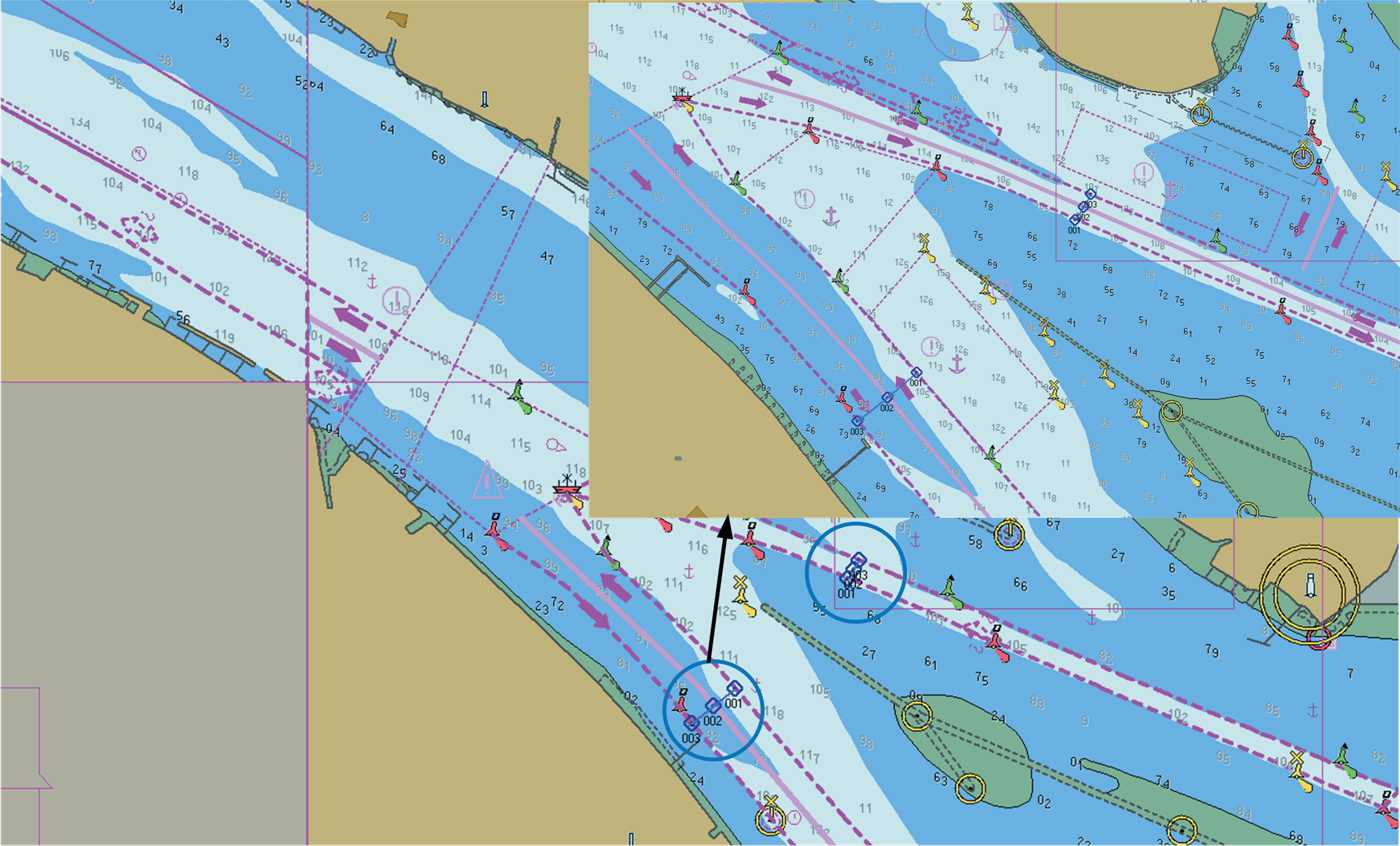
Figure 2. Waterway layout of Shanghai estuary of the Yangtze River.
A detailed shipping route chart is shown in Figure 2. The blue lines indicate two bottleneck points of this shipping channel. The width of the bottleneck to the northwest is 642·1 metres and the width of bottleneck to the southwest is 659·4 metres. According to government regulations, the maximum sailing speed allowed in this area is 11 knots and no overtaking manoeuvres are allowed.
4.2. Ship characteristics
In this study, AIS data from the Shanghai estuary of the Yangtze River was collected in March and April 2014. According to the collected AIS data, information including ship length, ship type, ship speed, ship course, latitude and longitude positions can be extracted. It should be pointed out that there may be some errors in the AIS data. For example, the AIS data report that some ships have extremely large ship lengths, which is obviously inconsistent with reality. Therefore, the procedure proposed by Qu et al. (Reference Qu, Meng and Li2011) was adopted to clean the errors of the AIS data. A total of 8,826 ships’ data was collected, including almost all ship types, including oil tankers, cargo ships, bulk carriers, passenger/Roll-On Roll-Off (RORO) ships, container ships, chemical carriers, tugs, fishing vessels, small boats and others.
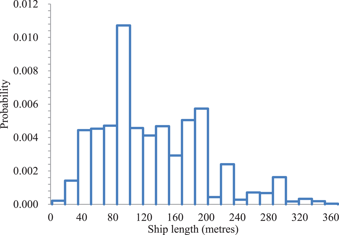
Figure 3 presents the length distribution for the 8,826 ships. It can be seen from Figure 3 that the majority of ships have lengths between 40 metres and 240 metres. It should be pointed out that the length of each ship type generally has considerable differences. As shown by Equations (2) and (3), the ship domain is significantly affected by the ship length. Therefore, there is a critical need to determine the ship classification in terms of ship length. In this study, the optimum number of ship groups in terms of ship length can be determined using the Centroid Clustering (CC) algorithm. In the CC algorithm, the objective function is to minimise the sum of the squared distances from the group means. The algorithm terminates when the number of iterations arrives at the pre-set maximum value. The optimum number of groups is found to be six: Group 1 (0, 40 metres], Group 2 (40 metres, 80 metres], Group 3 (80 metres, 160 metres], Group 4 (160 metres, 240 metres], Group 5 (240 metres, 320 metres] and Group 6 (320 metres, 369 metres]. Table 2 presents descriptive statistics of the ship lengths in these six ship groups. It can be found that the majority of ships in Group 1 are fishing vessels and tugs. Cargo ships and bulk carriers are the major ship types in Groups 1–3, as shown in Table 2.

Figure 3. Distribution of ship lengths extracted from the AIS data.
Table 2. Ship groups characterised by different ship lengths.
* I-Tanker, II-Cargo ship and Bulk Carrier, III-Passenger ships and Roll-on/Roll-off, IV-Container ship, V-Others (for example, tugs, fishing vessels).
# This refers to the total number of AIS records for the specific ship type during the analysis two months’ period.
4.3. Adjustment factors for ship domain
In order to investigate the effects of ship speed, ship type and time on the ship domain, a questionnaire survey of 80 ship captains and crew members was conducted. Each ship captain or crew member had an average of 6·14 years of navigation experience (standard deviation = 3·75 years). With the collected 80 sets of questionnaire survey results, the parameters shown in Equations (2)–(3) can be determined using the least squares error method, which are  $\alpha_{1}=5{\cdot}1504$,
  $\alpha _{2}=2{\cdot}2073$,
  $\beta _{1}=0{\cdot}1854$,
  $\beta _{2}=0{\cdot}1854$,
  $\gamma _{1}=0{\cdot}4458$,
  $\gamma_{2}=0{\cdot}1911$,
  $\delta _{1}=0{\cdot}4128$,
  $\delta_{2}=0{\cdot}1769$,
  $\varphi _{1}=0{\cdot}4596$,
  $\varphi _{2}=0{\cdot}1970$,
  $\tau_{1}=0{\cdot}2298$ and
  $\tau _{2}=0{\cdot}0985$, respectively. The positive signs for β 1, β 2, γ 1 and γ 2 shows that the ship domain size for oil/gas/chemical tanker and bulk carrier/general cargo ships is generally bigger than that for the tug, fishing vessel or small boats. In addition, these results also demonstrate our argument that a smaller ship domain is associated with the daytime period and slower sailing speeds.
5. RESULTS AND DISCUSSIONS
5.1. Capacity of waterway traffic composed of single ship type
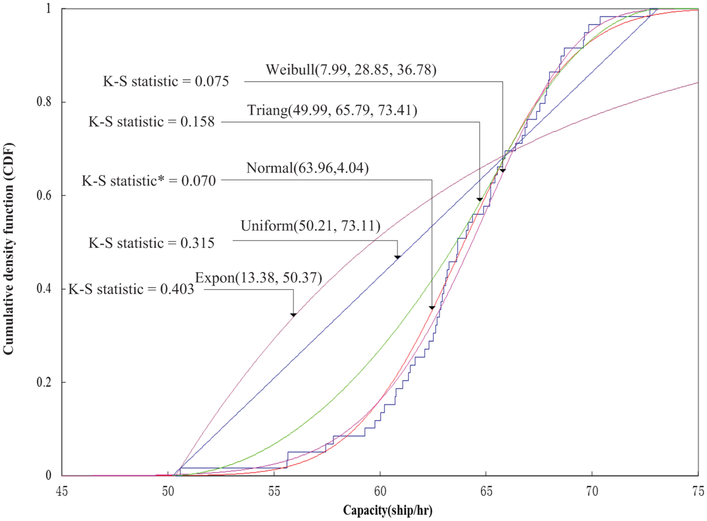
In order to reflect the uncertainty associated with the waterway traffic capacity mentioned above, the waterway traffic capacity should be represented by means of a probability distribution whose parameters can be determined based on the observed capacity data according to Equation (8). For example, one scenario assumes that the waterway traffic is only composed of cargo ships/bulk carriers with lengths between 80 metres and 160 metres. The best-fitted capacity distribution for this scenario is the normal distribution: Norm (63·96, 4·04) because the corresponding K-S statistic is lower than those from other four distributions, as shown in Figure 4.

Figure 4. Cargo ship/bulk carrier capacity distribution in Group 3.
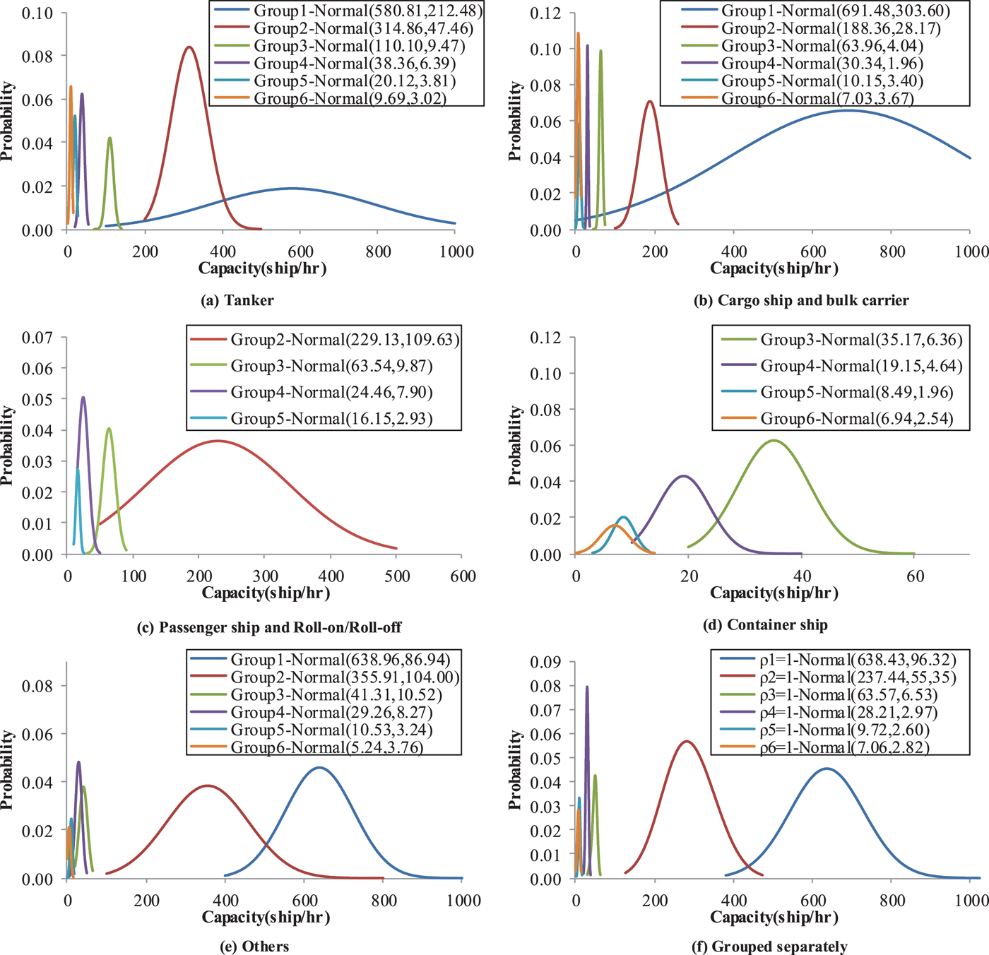
Five scenarios where waterway traffic is composed of only one ship type are now analysed: (a) tanker; (b) cargo ship/bulk carrier; (c) passenger/ roll-on roll-off ship; (d) container ship; and (e) others. Figure 5 shows the capacity distributions for these five scenarios. As can be seen from the figure, for each ship type, the maximum number of ships (for example, passenger/RORO ship) allowed to sail through the Shanghai estuary of the Yangtze River decreases significantly with the ship size (from Group 1 to Group 6). In reality, the waterway traffic would not be composed of only one ship type. Therefore, a more realistic scenario that the waterway traffic composed of various ship types is created. Figure 5(f) presents the capacity distribution for this more realistic scenario. Similar to Figures 5(a)–5(e), Figure 5(f) also shows that more small-sized ships (for example, Group 1) are allowed to sail through the waterway. For example, there is a capacity of 638·43 ships per hour for the waterway traffic composed of various types of ships less than 40 metres, while it is reduced to 7·06 ships per hour for the waterway traffic composed of ships larger than 320 metres.

Figure 5. Capacity distribution for different ship types.
5.2. Ship equivalent unit (seu) from the capacity viewpoint
As mentioned above, due to the unique ship characteristics, the maximum number of ships that can sail through the waterway link varies with different ship sizes. Therefore, it is of utmost importance to calculate how many benchmark ships equal to one ship in terms of waterway traffic capacity. For simplicity, the ships having lengths between 40 metres and 80 metres in Group 2 are considered as the benchmark ships in this study. Table 3 presents the ship equivalent units for different ship groups characterised by various ship lengths. It can be clearly seen from the table that the ship equivalent unit for ship Group 6 is the largest, followed by ship Group 5. Consistent with our expectation, it is also found that the ship equivalent unit could be affected by the time of day, as shown in Table 3. This might be because the waterway traffic capacity could be affected by the time of the day. For example, a one-way Analysis of Variance (ANOVA) test results show that the average maximum number of ships with lengths between 240 and 320 metres allowed to sail along the waterway is 33·2 ships per hour during the daytime period, which is statistically larger than that during the night-time period (27·2 ships per hour) at a significance level of 0.05. Therefore, one large-sized ship in Group 5 (i.e., 240metres<length≤320metres) equals 28·94 benchmark ships (for example, the ship length ranging from 40 metres to 80 metres) during the daytime period. However, a large-sized ship in Group 5 is only equivalent to 25·90 benchmark ships at night. The smaller equivalent unit of a ship with large-sized ship length at night may be explained by the fact that a large-sized ship will sail along the waterway at a slower speed during the nighttime.
Table 3. Ship equivalent unit in terms of waterway traffic capacity.
* Ships of Group 2 are considered to be benchmark ships.
5.2.1. Effects of the high proportion of large-sized ships on the mean of waterway traffic capacity
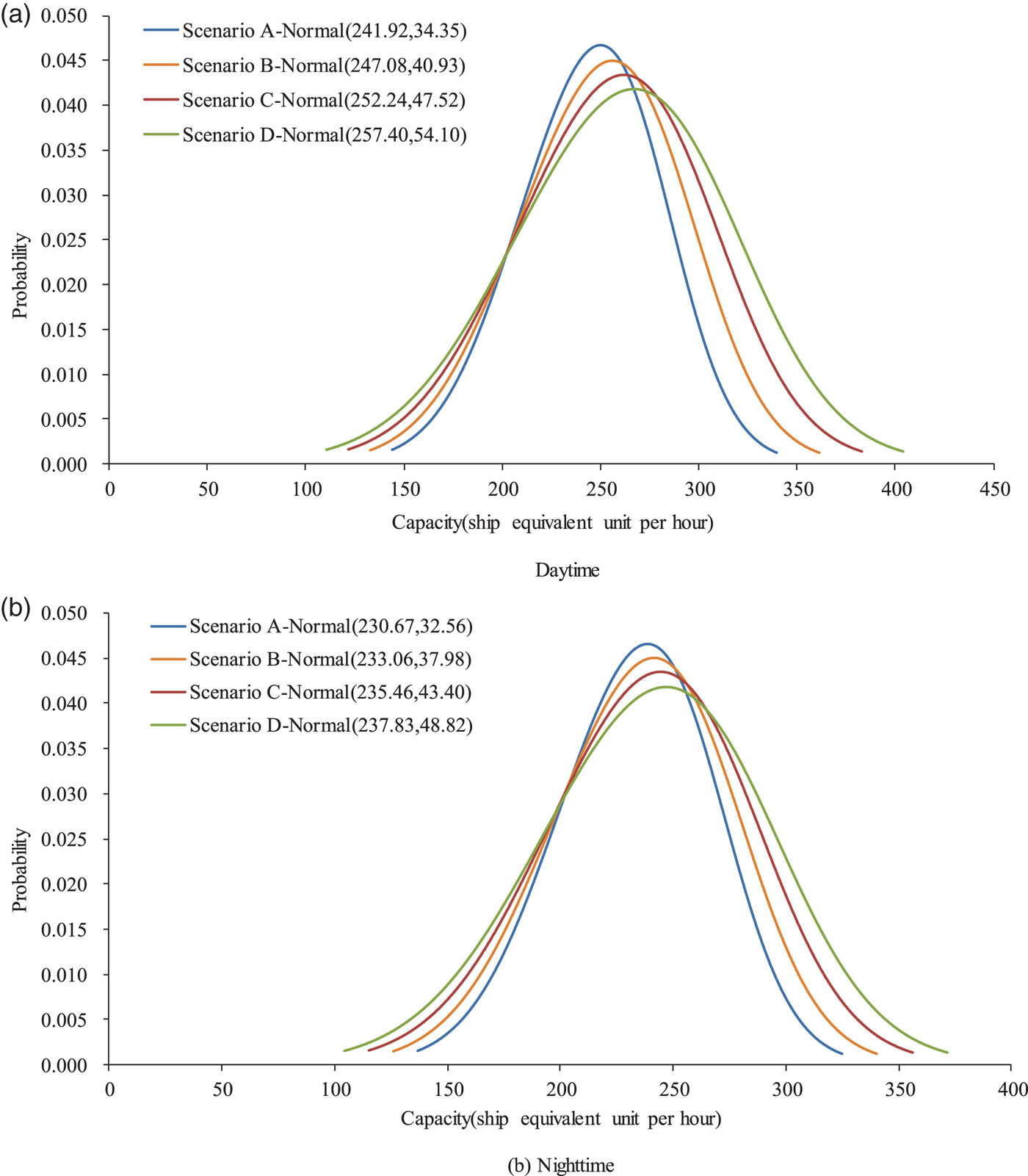
In reality, the waterway traffic would not be composed of only one type of ship with the same ship size. Realistic waterway traffic is composed of various ship groups with different proportions. For the sake of presentation, the scenario with observed ship compositions is considered as the benchmark scenario. Table 4 gives four scenarios for examining the effects of large-sized ships on waterway traffic capacity. Scenario A is considered as the benchmark scenario, where ship compositions are calculated according to ship voyages extracted from the archived AIS data. For example, the total number of voyages for ships in Group 1 accounts for about 12·64% of the total number of voyages. For voyages under Groups 2–6, the proportions are 8·14%, 52·87%, 20·68%, 4·86% and 0·81%, respectively. As mentioned before, the average ship size has been increasing rapidly (Zheng and Yang, Reference Zheng and Yang2016). In order to reflect the fact of an increasing proportion of large-sized ships, we further assume that the proportions of large-sized ships in Groups 5–6 increase by 5%, 10% and 15% in Scenarios B, C and D, respectively. The proportions of ships in other groups decrease proportionally for these three scenarios.
Table 4. Scenario design of ship traffic composition.
* Scenario A is designed based on the archived AIS data in March and April, 2014.
Figure 6 presents the capacity distribution of waterway traffic in four scenarios associated with different proportions of large-sized ships. It can be clearly seen from Figure 6(a) that the use of large-sized ships could increase the waterway traffic capacity. More specifically, the mean capacity for Scenario D is 257·4 seu/hr (that is, ship equivalent unit per hour), which is larger than that for Scenario A by 6·4% during the daytime period. Similarly, Scenario D also has an 8·2% larger capacity during the night-time period, as compared with Scenario A. In addition, Figure 6 also shows that the increment of waterway traffic capacity also increases with the proportion of large-sized ships. This provides adequate support for the argument that the deployment of larger ships will increase the capacity of a busy waterway.

Figure 6. Distribution of waterway traffic capacity under four different scenarios.
5.3. Effects of the high proportion of large-sized ships on the uncertainty of waterway traffic capacity
In order to measure the uncertainty of waterway traffic capacity caused by external stochastic factors such as unknown weather conditions, the confidence interval of waterway traffic capacity that is traditionally described as a range around the mean of the data can be determined (Weng and Yan, Reference Weng and Yan2016). In general, the Confidence Interval (CI) can be calculated by:
 $$CI_{\alpha}=[U-w_{\alpha},U+w_{\alpha}]$$
where U is the mean of waterway traffic capacity and w α is the absolute difference between the mean and lower bound of waterway traffic capacity at the confidence level of α.
Using Equation (9), the confidence interval of waterway traffic capacity can be easily determined. Figure 7 tabulates the CIs at various confidence levels for the four scenarios. It can be seen that the CI of waterway traffic capacity in Scenario A is [233·15 seu/hr, 250·69 seu/hr] at a confidence level of 95% and [236·78 seu/hr, 247·06 seu/hr] at a confidence level of 75%. This implies that the probability of waterway traffic capacity falling within a range from 233·15 seu/hr to 250·69 seu/hr is 0·95 in Scenario A. It can be found that confidence interval length increases with the proportion of large-sized ships at any specific confidence level. For example, the waterway traffic capacity in Scenario D has the widest confidence interval. Considering the fact that one large-sized ship is equivalent to a number of small-sized ships, it is apparently easier for maritime authorities to guide the large-sized ship operations. Actually, if the large-sized ships are not converted into the benchmark ships (that is, small-sized ships), the difference between upper and lower bounds of waterway traffic capacity is the smallest for Scenario D (only 13·8 ships/hr) at a confidence level of 0·95. This suggests that the deployment of large-sized ships could provide a more stable waterway traffic capacity prediction that is more helpful for maritime authorities to check the viability of waterway proposals in master planning of the Yangtze River.
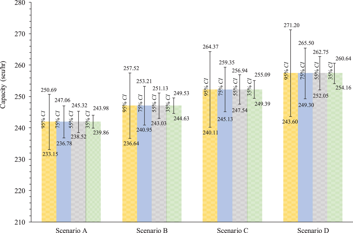
Figure 7. CIs at various confidence levels for the four scenarios.
6. CONCLUSIONS
This study proposed an efficient methodology to determine waterway traffic capacity at the Shanghai estuary of the Yangtze River considering dynamic ship domains. First, a calculation method based on the distribution of the MDTC was proposed to determine the observed waterway traffic capacity. Second, considering the possible effects caused by unknown factors like weather conditions, the waterway traffic capacity was further represented by a probability distribution rather than a single number in this study. Using the proposed methodology, the equivalent units of the ships with various ship sizes as well as the possible effects of large-sized ships on the waterway traffic capacity were examined. The results show that a large-sized ship is equivalent to more small-sized ships during the daytime period than at night. In addition, it was also found that the deployment of large-sized ships could increase the waterway traffic capacity at the Shanghai estuary of the Yangtze River. Moreover, the increment of waterway traffic capacity depends on the increased proportion of large-sized ships in the waterway link.
It is worth mentioning that the waterway traffic capacity is estimated based on the assumption that all ships should keep the MDTC and have no violations of their safety domain when it reaches capacity. However, ships may have dynamic interactions and influences on each other in reality. In this situation, it is very difficult to determine whether the waterway traffic estimate is exactly close to the true value. Future study will adopt traffic simulators to determine the effects of ship interaction on the waterway traffic capacity. Due to data limits, the effect of visibility on the waterway traffic capacity has not been taken into account though time of the day has partially captured the effect of this factor. The effect of visibility will be examined in the future after collecting more data.
FINANCIAL SUPPORT
This study is supported by the National Natural Science Foundation of China (Grant No. 71871137), also sponsored by Shanghai Education Development Foundation and Shanghai Municipal Education Commission (Grant No. 16SG41).