2.1. Statistical relationship between parameters

The core-distance of an object p in the method presented here is the distance to the minPts closest point, which is a concept in the OPTICS (Ordering points to identify the clustering structure) algorithm (Ankerst et al., Reference Ankerst, Breunig, Kriegel and Sander1999), written as Dist(minPts). In the ideal result of density-based clustering, all data in the high-density area should be grouped such that the density of the cluster can reach its maximum. From a local perspective, for an individual data point p, in the case of clustering with the centre data by itself given the fixed minPts, the core distance of p Dist(minPts) can exactly meet the conditions of a core point and cluster formation. Therefore, we believe that for a fixed minPts, the value of the core distance in this dataset that can enable the most point data to become core points is the appropriate parameter ε. Therefore, we use the inverse Gaussian distribution to find the mode value of the core distances and treat it as the appropriate parameter ε in this dataset when minPts is given. The formulae for the probability density function of the inverse Gaussian distribution and its mode value are given as follows:

(1)$$\hbox{P}\lpar x\rpar = \left[\displaystyle{{\lambda}\over{2\pi x^3}}\right]^{\displaystyle{{1}\over{2}}}e^{-\displaystyle{{\lambda \lpar x-\mu \rpar ^2}\over{2\mu^2x}}} $$

(2)$$Mode =\mu \left[\left(1+\displaystyle{{9\mu^2}\over{4\lambda^2}}\right)^{\displaystyle{{1}\over{2}}}-\displaystyle{{3\mu}\over{2\lambda}}\right]$$

where λ and μ can be obtained by Maximum Likelihood Estimate (MLE).

Because the parameter minPts ranges from one to the size of the dataset, based on the statistical relationship above, we can obtain all of the parameter combinations.

2.2. Selection of parameter combination

The clustering process is conducted with all of the parameter combinations and the number of outliers is taken as the clustering performance to select the optimum parameter combination.

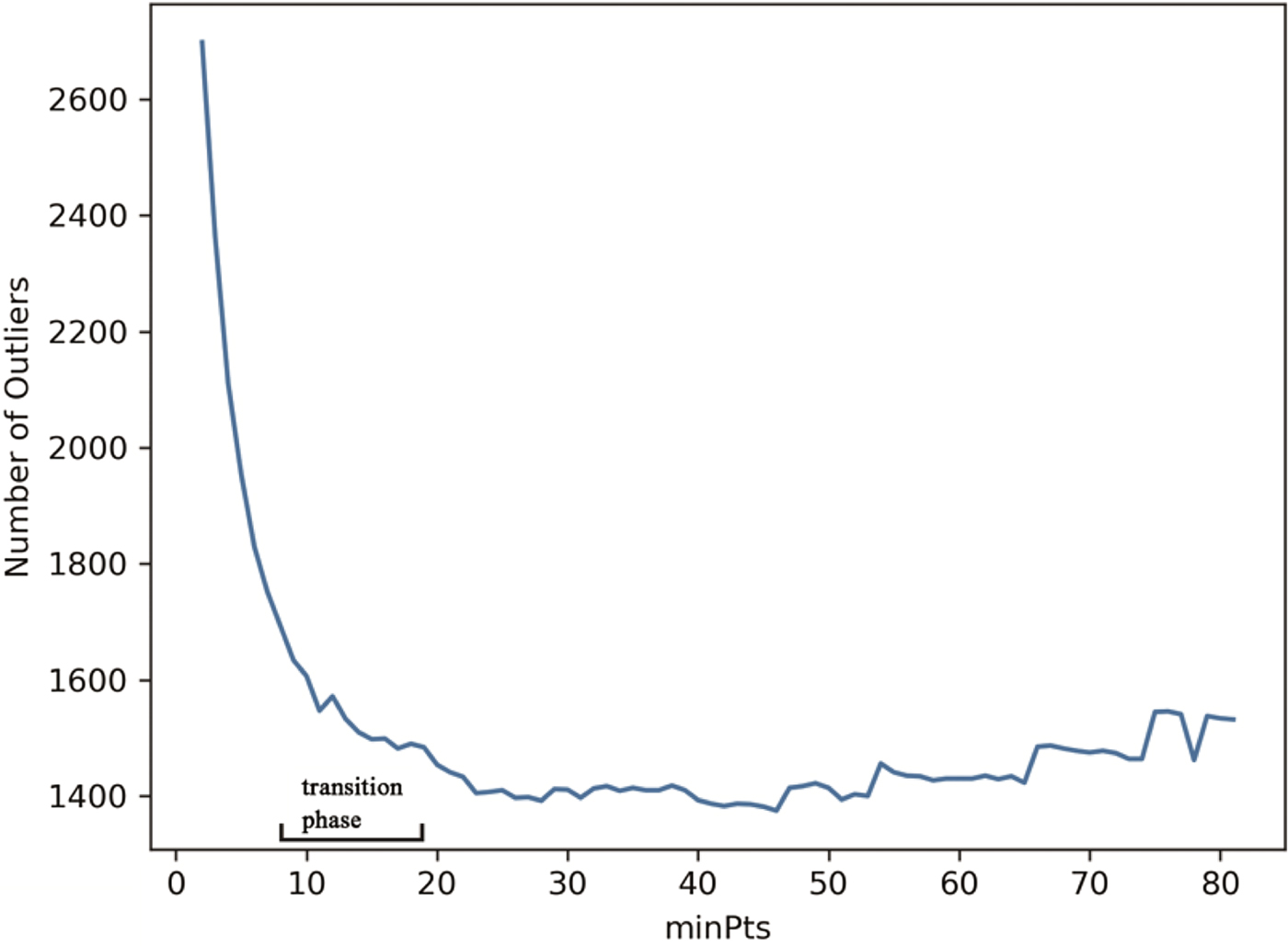
A parameter combination (minPts and its ε) corresponds to a certain degree of strength that can aggregate the elements into the clusters. A higher value of minPts indicates a greater strength. In multiple experiments, the change in the clustering result during the process of increases in the value of minPts can be viewed as a process in which each cluster absorbs the data around it. When minPts is equal to one, all data are classified as a cluster, and no outliers remain, which is apparently not appropriate. Thus, the process of increasing minPts is started at two, and at the beginning, many outliers occur around the clusters. With the increasing value of minPts, before the ideal clustering results are found, outliers are significantly absorbed into the clusters, which contributes to the sharp drop in the number of outliers. However, the outliers around the clusters subsequently become sparser. Hence, the reduction rate of the number of outliers decreases, which means that the number of outliers becomes stable.

Thus, we believe that the optimal parameter of minPts occurs at the transition phase from the stage of significant absorption of outliers to the stage of slowly absorbing outliers. In our method, we use a line graph of the number of outliers (in ascending order of minPts) to find the transition phase, as illustrated in Figure 1. Figures 1(a)–(d) show the clustering results with different parameter combinations (ascending order). The dotted-line circle represents the area of the corresponding ε of minPts. The number of outliers is plotted on the line graph, as illustrated in Figure 1(e). From Figure 1(e), minPts = 4 is identified in the transition phase. As shown in Figure 1(b), the clustering result with the corresponding parameter combination (minPts = 4) has exactly the ideal clustering performance.

Figure 1. The process of determining the parameter combination of DBSCAN algorithm. (a)–(d) Show the clustering results with different parameter combinations (ascending order). (e) Is the line graph for identifying the transition phase and optimal parameters.

3.1. Method of maritime anomaly detection based on RNN

The artificial neural network is one of the most effective data-driven approaches for the supervised learning task. It infers a function that maps an input to an output based on example input-output pairs derived from existing data. The characteristics can be used for anomaly detection, not only because it can predict the trajectories that conform to historical patterns, but also for the trajectories that did not conform to historical patterns it may sensitively become inefficient in prediction. While the latter is the property that other trajectory prediction methods that do not rely on historical data, such as the Kalman filter (Perera and Soares, Reference Perera and Soares2010; Stateczny and Kazimierski, Reference Stateczny and Kazimierski2011), do not have. Compared to those methods, a neural network can store the trajectory information in the customary route, which is extracted from historical data; only the regular ship movement can be predicted accurately. In the prediction that does not rely on historical data, the goal is to predict the vessel trajectory as accurately as possible no matter whether the movement is abnormal or not. This is the reason the neural network is applied as the predictor in this research, which has different predictive effects for different degrees of abnormality.

An RNN is a class of artificial neural network in which connections between nodes form a directed graph along a sequence. RNNs can use their internal state (memory) to process sequences of inputs. This process allows the model to learn temporal behaviours in a time sequence. The basic principle of the method presented here is that an RNN trained by trajectory data from the results of the DBSCAN algorithm is used as a vessel trajectory predictor. According to the previous tracking points and the traffic pattern, the network can predict the normal position of the next tracking point. It is hypothesised that anomalous vessel behaviours regarding vessel speed, course and route can cause abnormal performance in vessel position. Here, anomalous vessel behaviours are identified through the detection of abnormal position, and the deviation value between the predictive position and actual position is the indicator that shows the normality degree of the tracking point, defined by:

(3)$$deviation\_value=GeoDistance\lpar Lat_{pre}\comma \; Long_{pre}\comma \; Lat_{act}\comma \; Long_{act}\rpar $$

where GeoDistance is the function for calculating the geographical distance between two geographical coordinates. Lat _pre and Long _pre are the geographical coordinates of the predictive position. Lat _act and Long _act are the geographical coordinates of the actual position.

To supply a warning, the thresholds of the deviation value can be determined based on the user's practical requirements and the performance of training. The method here sets high and low levels of thresholds. New vessel position data generates a warning to attract additional attention from supervisors when the deviation value exceeds the high level or when the deviation value has exceeded the low level for several consecutive tracking points as these situations might be the anomalous vessel behaviours. In contrast, new vessel position data are treated as normal vessel behaviour when the prediction of the network is accurate.

The trajectories can be described by a set T = {t _i|t _i, i = 1,…2,n}, where t is the trajectory in the experiment and n is the number of trajectories. Trajectory data t consists of AIS tracking points, defined by:

(4)$$t=\lcub p_j \vert p_j=\lpar x_j\comma \; y_j\comma \; v_j\comma \; c_j\rpar \comma \; \ j=1\comma \; 2\comma \; \ldots\comma \; m\rcub $$

where j is the time instance index, m is the total number of tracking points in the trajectory and p _j is the state vector of the ship at time index j. For the state vector, x _j and y _j are the coordinates of the tracking point and v _j and c _j are the speed and course of the ship at time index j. In addition, the values were normalised before training of the RNN. Feature scaling is used to bring all values into the range [0, 1].

Trajectory data were processed into input and output datasets by a sliding window for the neural network. The processing method is shown in Algorithm 1.

Algorithm 1. Creation of a dataset for the neural network

3.2. RNN and long short-term memory

Compared to the traditional structure of a neural network, namely feed-forward neural network, the training efficiency of an RNN is higher in processing time series data. When applying a feed-forward neural network in the prediction of time series data, a fixed time step of information vectors of track points is concatenated into a larger vector by windowing. The information flow from the input layer to the hidden layer is shown in Figure 2. The hidden node value h is calculated as Equation (5).

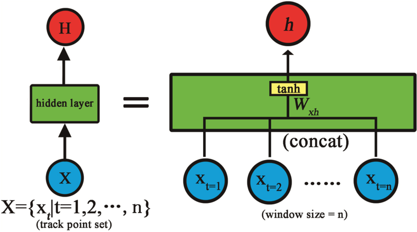
Figure 2. Information flow in a feed-forward neural network.

(5)$$h=tanh\ \lpar W_{xh} \cdot\, concat\, \lpar x_1\comma \; x_2\comma \; \ldots\comma \; x_n \rpar +b\rpar $$

With a single training example, the weight of feed-forward neural network W _xh can be trained by information at all the time steps only once. While in the RNN, the parameters are shared by all time steps, which may increase the training efficiency sharply. The basic structure of our RNN is shown in Figure 3.

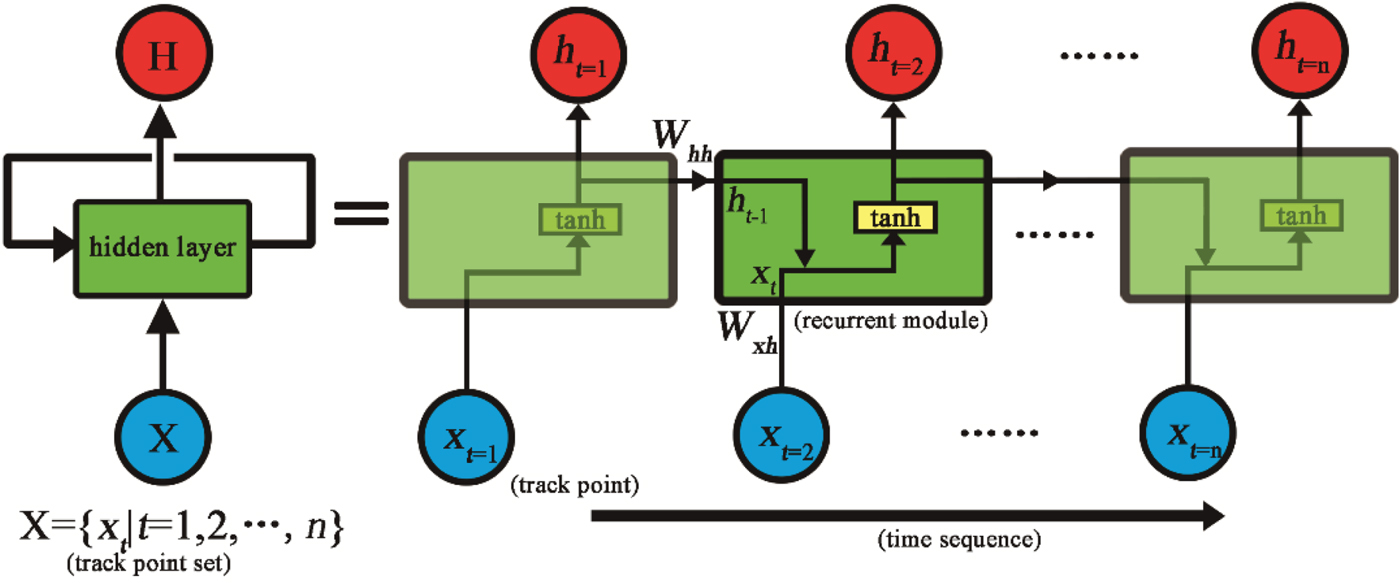
Figure 3. Information flow in a recurrent neural network.

As shown in Figure 3, the training of each moment is independent. At time t nodes with recurrent modules receive input from the current data point x _t and from the hidden node value h _t−1 in the previous state. At time t, nodes with recurrent modules receive input from the current data point x _t and from the hidden node value h _t−1 in the previous state. The hidden node value h _t at time t is calculated as Equation (6). That is to say, RNNs share weights across different time steps of the sequence. Consequently, if there are n time steps in the input data, with a single training example, the weights of RNN W _xh, W _hh can be trained n times.

(6)$$h_t =tanh \lpar W_{xh} \cdot x_t +W_{hh} \cdot h_{t-1} +b\rpar $$

In this paper, prediction of the vessel trajectory is performed by a fully connected RNN. A single hidden layer is used, and the number of hidden dynamic features of the hidden layer is determined based on the input data. In updating the weights, the Adam algorithm is applied (Kingma and Ba, Reference Kingma and Ba2014); this is a method for efficient stochastic optimisation that requires only first-order gradients and has low memory requirements. The method computes the individual adaptive learning rates for different parameters from estimates of the first and second moments of the gradients. Additionally, the model uses the Rectified linear unit (Relu) as the activation function (Nair and Hinton, Reference Nair and Hinton2010).

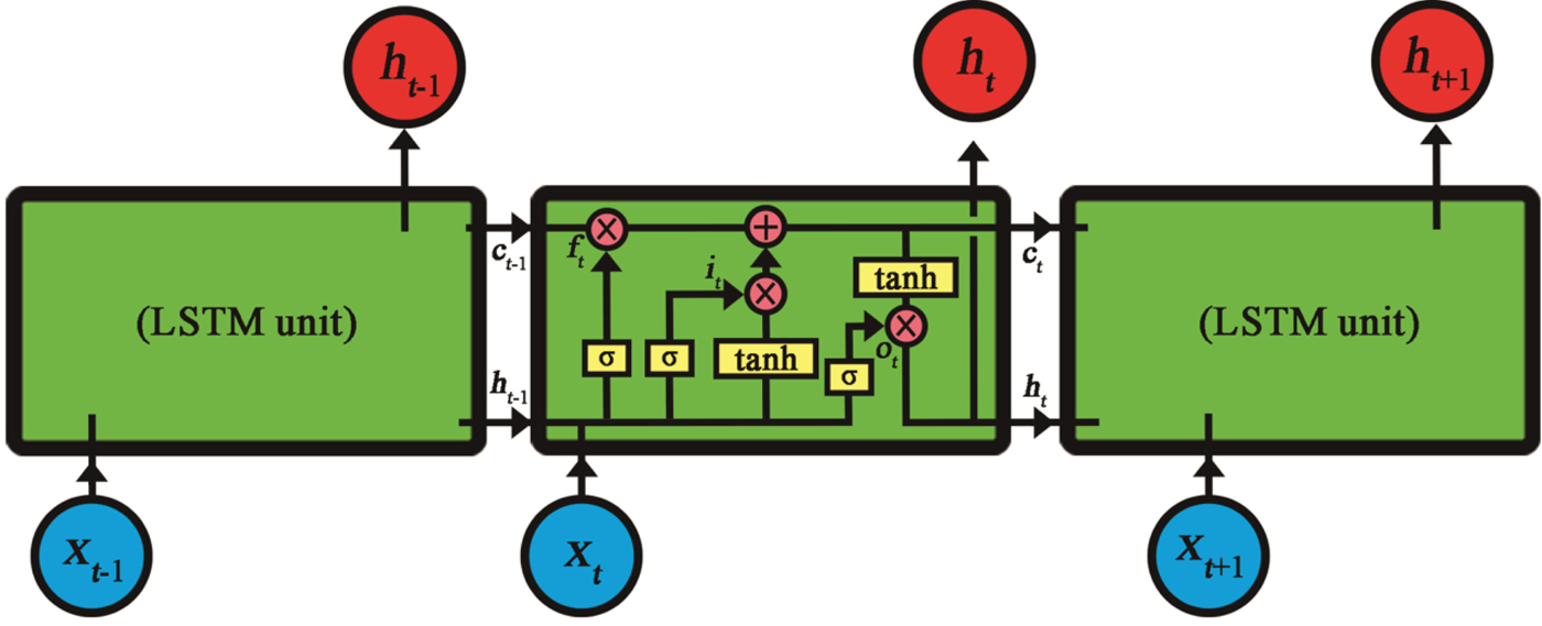
One of the most successful RNN architectures for sequence learning was introduced to solve the problem of vanishing gradients, namely, the Long Short-Term Memory (LSTM) (Hochreiter and Schmidhuber, Reference Hochreiter and Schmidhuber1997). In this method, the traditional nodes in the hidden layer are replaced with the LSTM unit, which is shown in Figure 4.

Figure 4. Information flow in a recurrent neural network with LSTM unit.

The key to the LSTM unit is the cell state. The cell state c _t at time t is shown as the horizontal line running through the top of the LSTM unit in Figure 4. The LSTM unit has the ability to remove or add information to the cell state through the gates, which are marked with f _t, i _t, and o _t in Figure 4. Gates are a way to optionally let information through and are composed of a sigmoid neural net layer (marked with σ) and a point-wise multiplication operation (marked with a multiplication symbol). f _t indicates the forget gate, which decides what information should be discarded from the cell state. The process looks at h _t−1 and x _t, and outputs a number between 0 and 1 for each number in the cell state C _t−1. The number 1 represents “completely retain this”, whereas the number 0 represents “completely discard this”. Additionally, i _t indicates the input gate, which decides what new information from h _t−1 and x _t can be stored in the cell state, and o _t denotes the output gate, which decides how much information in the cell state can be output. The equations of these gates are shown as follows:

(7)$$f_t = sigmoid\lpar {W_{xf} x_t +W_{hf} h_{t-1} +b_f } \rpar $$

(8)$$i_t =sigmoid\lpar {W_{xi} x_t +W_{hi} h_{t-1} +b_i } \rpar $$

(9)$$o_t =sigmoid\lpar {W_{xo} x_t +W_{ho} h_{t-1} +b_o } \rpar $$

Finally, the cell state c _t at time t is calculated based on the gates (f _t and i _t), input x _t, previous cell state c _t−1 and previous hidden node value h _t−1. The hidden node value h _t at time t is calculated based on cell state c _t and output gate o _t. The equations of c _t and h _t are shown as follows:

(10)$$c_t =f_t \odot c_{t-1} +i_t \odot tanh\lpar {W_{xc} x_t +W_{hc} h_{t-1} +b_c } \rpar $$

(11)$$h_t =o_t \odot tanh\lpar {c_t } \rpar $$

4.1. Experimental setup

AIS data was collected from the Zhoushan Islands in January 2015. The research area is located outside of Beilun-Zhoushan port, which is one of the most important ports in China. This water area is situated near the middle portion of the China coastline. Many vessels that use the north-south transportation routes sail through this area. In addition, this area is close to the entrance of the Shrimp main gate waterway, which is the main waterway of Beilun-Zhoushan port, and thus, it is the main area where in-and-out of port ship encounters occur, as shown in Figure 5. All of the Class-A AIS messages from tankers and cargo ships were selected as experimental data from a total of 3,228 trajectories of 1,932 vessels. The data were pre-processed with respect to space and time (Zhao et al., Reference Zhao, Shi and Yang2018).

Figure 5. Experimental data source.

4.2. Results of vessel trajectory clustering

As described in Section 2.2, in the process of determining the parameter combination, the line graph of the number of outliers and the transition phase is shown in Figure 6. It is worth mentioning that there are slight increases in the noise levels in Figure 6. This is because in the process of increasing the value of minPt, when the merger of clusters occurs, the data around the edge of the original cluster might be identified as noise data. However, it does not affect the overall trend. After checking the clustering results with the parameter combinations in the transition phase, the parameter combination (minPt = 10, ε = 0.861) was determined. The results of the clustering for normalcy extraction are shown in Figure 7 and Table 1.

Figure 6. Line graph of the number of outliers in the experiment.

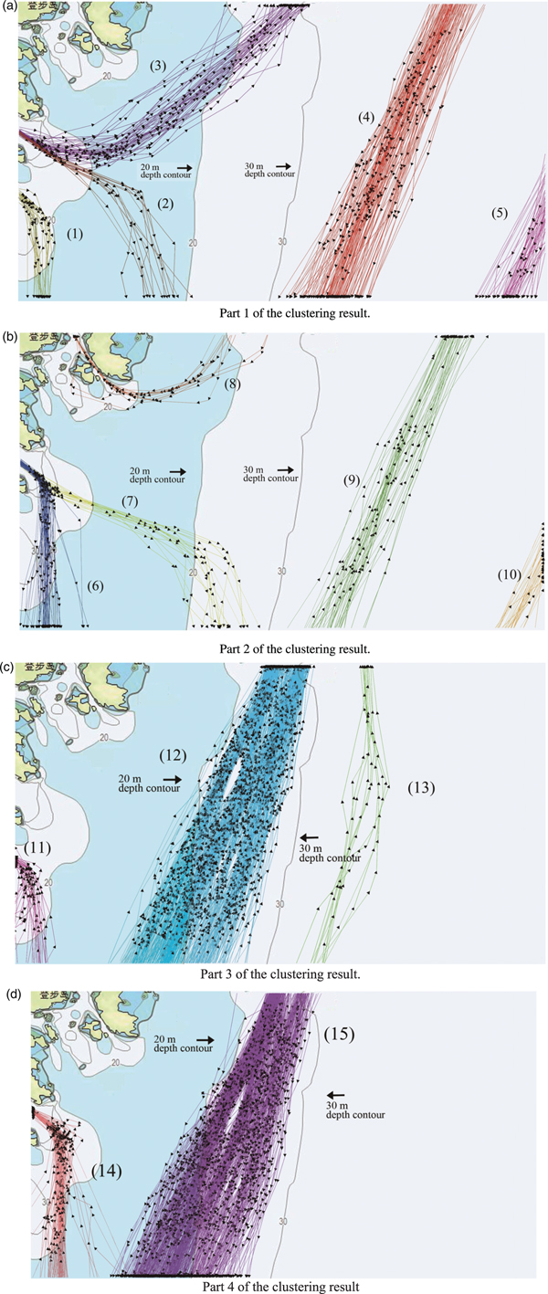
Figure 7. Results of proposed Density-based clustering.

Table 1. Description of clusters.

From Figure 7 and Table 1, it is shown that the vessel trajectories that belong to the different customary routes are grouped into different clusters. From observation, the vessel trajectories in the same cluster are almost consistent in terms of shape. Compared to the results of classification-based clustering (Figure 8), the noise trajectories are removed, and the meaning of the cluster is clearer. The results show that the DBSCAN algorithm with the proposed method for determining the parameters is able to recognise the traffic patterns on the water. Although not all of the customary routes in this experiment area were detected, the clusters consisting of vessel trajectories in the results can still be used as normalcy data for maritime anomaly detection.

Figure 8. Results of classification-based clustering.

4.3. Experiment on maritime anomaly detection using recurrent neural networks

As described in Section 3, the vessel trajectories in the results of the DBSCAN algorithm were used to train the recurrent neural network with the LSTM unit introduced in Section 3.2. The parameter used in the process of obtaining the training dataset, namely window_length, is determined as five, which means that in our method, the prediction of the tracking point is made based on five previous tracking points. The time interval of the tracking points in the data set was processed into two minutes. In other words, in this experiment, the method assesses whether the behaviour of the vessel is anomalous by comparing the position that was predicted two minutes ago with the actual current position. The deviation value between the predictive position and the actual position is the indicator used to evaluate results from the neural network.

4.3.1. Prediction of vessel position

First, a comparison experiment regarding the prediction performances of a feed-forward neural network (three-layer BP neural network) and recurrent neural network was conducted. The deviation values of these two neural networks after different training epochs are shown in Figure 9. Figures 9(a) and 9(b) are the comparison results of prediction error based on the training dataset and testing dataset (data other than the vessel trajectories contained in the training set), respectively. In this experiment, the testing dataset consists of the vessel trajectories that account for 15% in each cluster.

Figure 9. Comparison results of prediction error between BP neural network and recurrent neural network.

From Figure 9, it can be seen that after the same training epoch the average prediction error of the RNN is 12.8% (training dataset: 20%) below the error of the feed-forward neural network. It is shown that the recurrent neural network used here has a better performance regarding training efficiency and prediction accuracy compared to the feed-forward neural network.

In the verification experiment, the testing dataset was used to validate the ability to predict the normal vessel position and the ability to detect anomalous behaviours of the vessel.

As shown in Figure 9(b), after the prediction, the prediction error (the mean of all of the deviation values using the testing dataset) is 60 m, which can satisfy the accuracy needs of traffic surveillance. Three detailed results of prediction are shown in Figure 10. As shown in Figure 10(a), these three vessel trajectories are the normal trajectories that follow the traffic pattern in this water area, which are selected from the results of clustering. These vessel trajectories are all located in the customary route, and the movement of the ship is steady (no sudden change in course and speed). Figures 10(b)–(d) show that the position can be predicted with acceptable precision by the neural network that has learned normalcy. Consequently, the method has been proven to have the ability to predict the position where the vessel is expected to be according to the traffic pattern on the water.

Figure 10. Three detailed results of prediction and deviation value between actual position and actual position.

4.3.2. Detection of anomalous vessel behaviours

The vessel tracking points that do not follow the traffic pattern are treated as anomalous vessel behaviours. In marine traffic, the situations that might cause such mismatches include abnormal changes in course, abnormal changes in speed and sailing on an abnormal route. In this experiment, three types of abnormal vessel trajectories were selected to verify the detection capability. In the process of detection, two thresholds of deviation value of position were set to supply the forewarning signal, namely, 75 m (low level) and 250 m (high level). The detailed results are shown in

As observed from Figure 11(a), the trajectory is generated for a vessel that sails from the area in the south to the Shrimp main gate waterway for entry to the port. However, unlike most other vessels, which take a steady course, the course that is shown in this trajectory has changed several times within a short period (marked with a black block). The detailed predictive results in this period are shown in Figure 11(b). In Figure 11(b), the deviation value of the tracking point that has a sharp change in course is significantly larger than that of the others. Based on the thresholds of deviation, those tracking points (anomalous vessel behaviours) have been detected and are marked with a symbol. The detailed detection results in this period are shown in Table 2. The deviation between the actual position and predictive position that is caused by the sharp change in course exceeds the threshold value, which is identified as anomalous vessel behaviour.

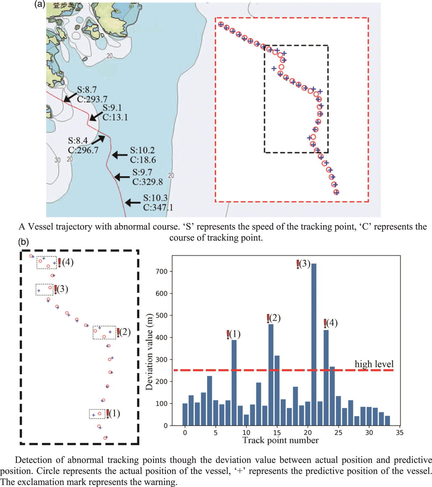
Figure 11. Detailed prediction result of vessel trajectory (abnormal course).

Table 2. Detailed detection result of vessel trajectory (abnormal course)

From Figure 12(a), it can be seen that the trajectory is generated for a vessel that sails from the port area to the water area in the north. However, in its movement process, the vessel slowed down and stopped for an hour (marked with a black block) near the entrance to the waterway. This anomalous vessel behaviour seldom occurs in this water area and might influence the traffic flow through the waterway. The detailed predictive results are shown in Figure 12(b). From Figure 12(b), in the area marked with ‘(1)’ and ‘(3)’, the sudden increase in deviation value was caused by the abnormal change in speed and course. Moreover, in the area where the vessel abnormally stopped (marked with ‘(2)’), the tracking points that have larger deviation values were detected for the warning state. The detailed detection results are shown in Table 3. The deviation between the actual and predictive positions that is caused by the abnormal change in speed exceeds the threshold value, which is identified as anomalous vessel behaviour.

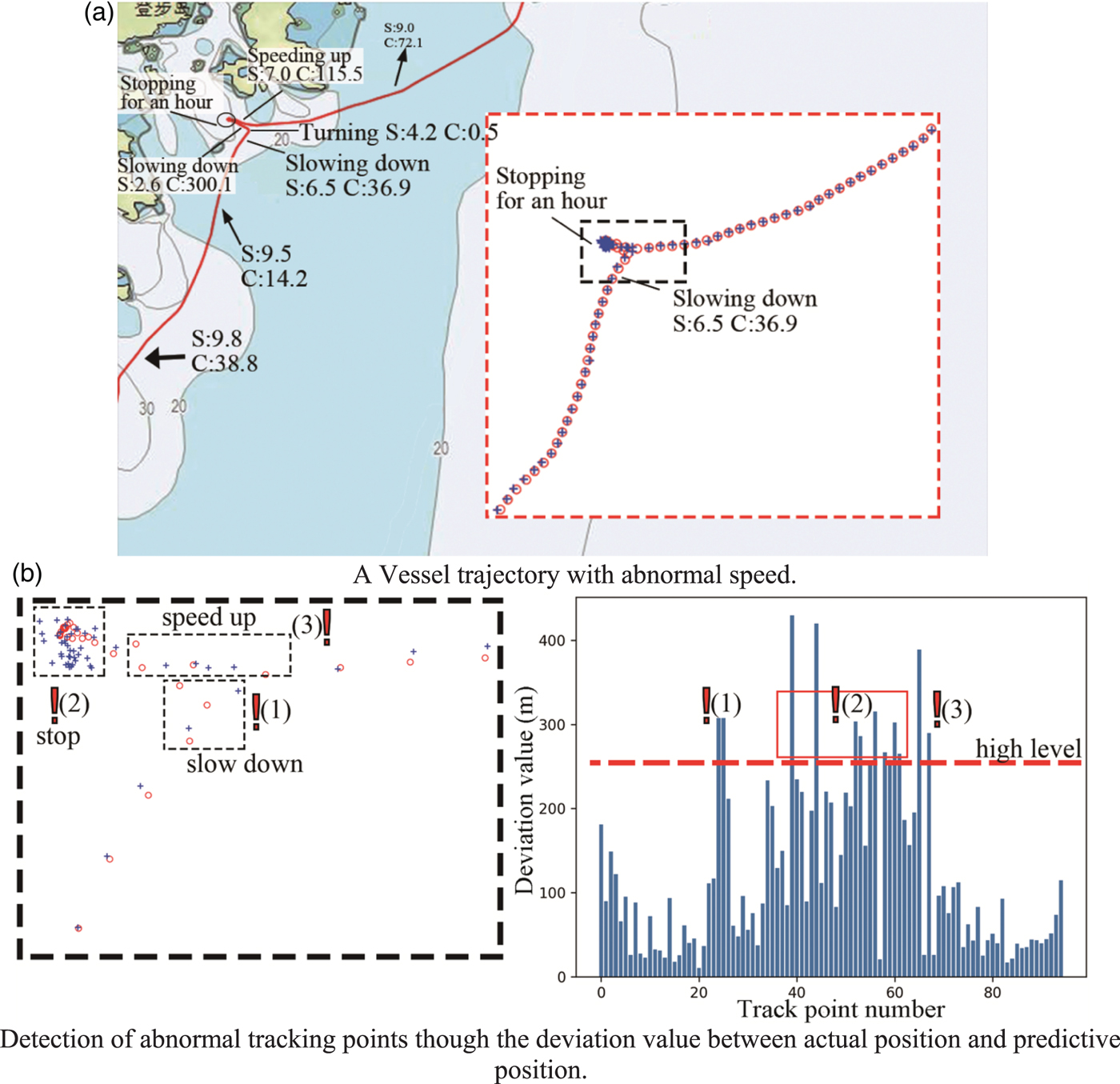
Figure 12. Detailed prediction and detection result of vessel trajectory (abnormal speed).

Table 3. Detailed detection result of vessel trajectory (abnormal course)

In Figure 13(a), the trajectory is generated for a vessel that sails from the Fuli gate waterway to the water area in the south. The first half of the vessel trajectory is a route that is not popular in this water area. The second half of the vessel trajectory follows the existing traffic pattern shown by the cluster (class 6) in the DBSCAN results. The detailed predictive results of the first half (marked with a black block) are shown in Figure 13(b). Due to the abnormal route, the deviation values of the tracking point in this region are all relatively large. Those tracking points that exceed the low level consecutively have been detected by our method (marked with a block in Figure 13(b)).

Figure 13. Detailed prediction and detection result of vessel trajectory (abnormal route).

This experiment shows that our method has the ability to detect the anomalous behaviours of a vessel in terms of speed, course and route within a short time.