


1. INTRODUCTION
Connected and Autonomous Vehicles (CAVs) have been researched extensively in recent years to solve current traffic issues and to realise the concept of an intelligent transport system. In theory, CAVs can improve road safety, reduce traffic congestion, reduce emissions from vehicles and save time during transportation (Atkins, 2016). CAVs are the combination of Connected Vehicles (CVs) and Autonomous Vehicles (AVs). CVs use different communication technologies to communicate with drivers, other cars on the road (vehicle to vehicle) and roadside infrastructure (vehicle to everything) (CAAT, 2016). AVs guide themselves without any human intervention by using technologies such as crash warning systems and lane keeping systems (Anderson et al., Reference Anderson, Nidhi, Stanley, Sorensen, Samaras and Oluwatola2016).
A well-developed positioning system is necessary for AVs to achieve full automation while driving. The system should provide high accuracy, mobility, continuity, flexibility and scalability (Meng et al., Reference Meng, Dodson, Moore and Roberts2007). High-precision Global Navigation Satellite Systems (GNSS) provide the required accuracy, availability and reliability, and is the only realistically viable solution for precisely tracking AVs on roads. Moreover, Network Real-Time Kinematic (NRTK) positioning is the most suitable positioning technique for AVs because it has a high accuracy and good mobility (Meng et al., Reference Meng, Dodson, Moore and Roberts2007; Aponte et al., Reference Aponte, Meng, Moore, Hill and Burbidge2008). NRTK positioning provides centimetre-level accuracy and is not affected by spatially correlated errors (Cai et al., Reference Cai, Cheng, Meng, Tang and Shi2011). However, high-performance equipment is too expensive for commercial use in CAVs; therefore, the use of a low-cost GNSS receiver to achieve real-time, high-accuracy and ubiquitous positioning performance may be a future trend (Cui et al., Reference Cui, Meng, Chen, Gao, Xu, Roberts and Wang2017).
This study evaluated the positioning performance of a low-cost receiver with a developed NRTK positioning system in a CAV driving environment.
The accuracy requirements of CAVs are categorised into the following four categories (Basnayake et al., Reference Basnayake, Williams, Alves and Lachapelle2010; Stephenson, Reference Stephenson2016):
• Which Road: Applications in this category typically require an accuracy of 5 m. This allows the system to locate a vehicle on a particular road, and this accuracy level can be used for journey planning, accident blackspot warning, environmental monitoring and congestion relief.
• Which Lane: Applications in this category require an accuracy of 1·5 m. This allows the system to locate the lane in which a vehicle is driving. This accuracy level can be used for applications in the “Which Road” category and for those requiring congestion charging, variable-speed adaptation, incident detection and emergency vehicle prioritisation.
• Where in Lane: Applications in this category require an accuracy of 0·5 m. This technique provides the appropriate position of a vehicle within the lane in which the vehicle is driving. This category is used for driving monitoring, precrash restraint deployment, collision avoidance and road condition monitoring.
• Active Control: Applications that require an accuracy better than 0·1 m are categorised here. At this accuracy level, vehicles are controlled actively, and applications include vehicle platooning, rollover prevention, autonomous vehicle control and automated road trains.
2. METHODOLOGY AND EXPERIMENTAL DESIGN
The developed NRTK positioning system used with a low-cost GNSS receiver (u-blox NEO-M8T) is based on RTKLIB (Takasu, Reference Takasu2013) and was implemented using Raspbian (Raspberry Pi Foundation) (Figure 1).

Figure 1. The developed NRTK Low-cost GNSS receiver. (Courtesy Raspberry Pi Foundation and U-blox UK)
A Raspberry Pi 3, a single-board computer that has a wireless Local Area Network (LAN) and Bluetooth connectivity and is powered by a Universal Serial Bus (USB) phone charger, was used in this study. It ran on a free operating system from a Secure Digital (SD) card. The cost of a Raspberry Pi 3 is approximately \pounds 30.
The NEO-M8T module supports the Global Positioning System (GPS), Globalnaya Navigazionnaya Sputnikovaya Sistema (GLONASS), BeiDou and Galileo constellations (GPS/Quasi-Zenith Satellite System (QZSS) L1 Coarse/Acquisition (C/A), GLONASS L10F, BeiDou B1 Satellite-based Augmentation System (SBAS) L1 C/A; Wide Area Augmentation System (WAAS), European Geostationary Navigation Overlay Service (EGNOS), Multi-functional Satellite Augmentation System (MSAS) and GPS-aided Geostationary Earth Orbit (GEO) augmented navigation (GAGAN) Galileo E1B/C). In addition, the module provides raw data used for further calculations through the NRTK technique, including code pseudo-range and carrier phase observations and navigation data. The NEO-M8T module costs approximately \euro 80.
A GNSS receiver module was embedded on the Raspberry Pi 3 and connected to a geodetic antenna (Figure 2). The low-cost receiver utilised the NRTK positioning technique, receiving corrections from SmartNet (a NRTK corrections service) through the Network Transport of Radio Technical Commission for Maritime Services (RTCM) through Internet Protocol (NTRIP), and provided position information at 1 Hz.

Figure 2. NRTK positioning program in the low-cost GNSS receiver configuration.
RTKLIB supports various positioning modes with GNSS for both real-time processing and postprocessing: Single, Differential GPS (DGPS)/Differential GNSS (DGNSS), Kinematic, Static, Moving-Baseline, Fixed, Precise Point Positioning (PPP)-Kinematic, PPP-Static and PPP-Fixed (Takasu, Reference Takasu2013). In this study, the kinematic mode in RTKLIB was utilised for data processing.
The system requires a configuration file, which contains input options, processing options and output options. The main settings are described in the following paragraphs.
Regarding input options, the u-blox NEO-M8T module was set as a rover input stream so that the system could receive raw observation data through a serial port. The system can recognise the raw observational data in the u-blox format for further calculations. The base input stream was set to connect to the Leica SmartNet server for the system to receive corrections in the RTCM3 format through the NTRIP. The MAX-RTCMv3 mounted point was used for the corrections of the data.
Regarding processing options, the frequency was set as L1 because the u-blox NEO-M8T supports only a single frequency for one satellite system. The “forward filter solution” filter type was used; ionospheric correction was based on the Klobuchar model (Takasu, Reference Takasu2013); tropospheric correction was based on the Saastamoinen model (Takasu, Reference Takasu2013); and the satellite ephemeris used was the broadcast ephemeris. The maximum value of the time differential between the rover and base station was set as 30 s, which is the toleration time of the internet connection delay.
Regarding output options, the solution format was set as latitude, longitude and height; the time system was set as GPS time; the datum was set as World Geodetic System (WGS) 84 and the height was ellipsoidal.
The positioning system built on the Raspberry Pi was based on the open source software RTKLIB. The system was implemented with two LEDs for system monitoring and a button for shutting down the low-cost receiver.
The experiments were conducted in Nottingham by using a Nottingham Geospatial Institute (NGI) van (Figure 3). There are two Inertial Navigation Systems (INS) installed in the van which are an Applanix POSRS INS and an ARGONAUT INS. The Applanix POSRS INS is more precise than ARGONUT INS, and it was used as the reference trajectory in the experiment.

Figure 3. NGI van.
The experiments were conducted on 19 June 2017 in Nottingham between 13:00 and 16:00 (GPS time) Figure 4 provides detailed information and Position Dilution of Precision (PDOP) values during the experiments.

Figure 4. PDOP values and number of satellites in the experiment.
The route of the trial is shown in Figure 5. The test environment included a rural area, motorway, an interurban area and an urban area. The range of this experiment is around 52°48′N, 1°18′W to 52°57′N, 1°06′W. By selecting this route design, we aimed to evaluate the general positioning performance of the low-cost receiver in each area.

Figure 5. Route of the experiment (mapped by ArcGIS).
As shown in Figure 6 the NGI van was equipped with a Leica AS10 antenna (Front Left, FL), a Novatel 703 GGG antenna (Rear Right, RR), a Tallysman 3970 antenna (Front Right, FR), two Leica GS10 receivers, the low-cost receiver, the POSRS INS and a low-cost Inertial Measurement Unit (IMU) (ARGONAUT). The kinematic testing data was collected by the Leica AS10 antenna, which was installed on the top of the van (FL position), and then received by the Leica GS10 (GS10-8) and low-cost receivers. The reference trajectory of the kinematic test was generated on the basis of the INS (POSRS), whose antenna was installed in the RR position.
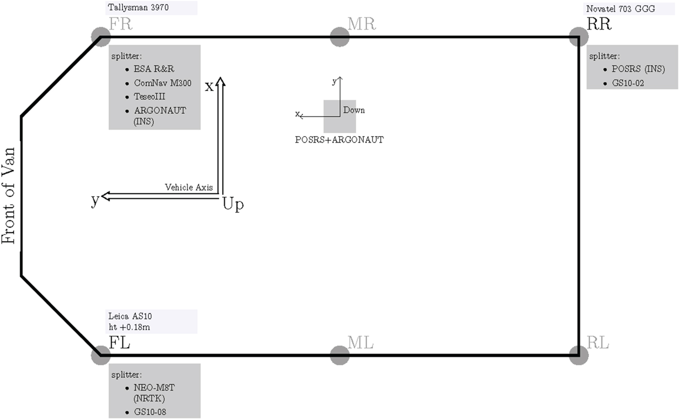
Figure 6. Equipment configuration for the experiment.
3. RESULTS AND DISCUSSION
The results are discussed with respect to five combinations: the low-cost receiver performing NRTK positioning in real time (u-blox+RTCM(RT)), the low-cost receiver performing NRTK positioning with correction during postprocessing (u-blox+RTCM), the geodetic receiver performing NRTK with correction during postprocessing (GS10+RTCM), the low-cost receiver performing baseline RTK with SUBO base station observations during postprocessing (u-blox+SUBO) and the geodetic receiver performing baseline RTK with SUBO base station observations during postprocessing (GS10+SUBO).
The positioning performance of the geodetic receiver and the low-cost receiver was first analysed, and the accuracy of the low-cost receiver was evaluated according to the accuracy requirements of CAV applications. Finally, the performance of the low-cost receiver in different areas was evaluated.
To accurately evaluate the positioning performance, outliers were excluded from all analyses except that of the CAV application accuracy requirements. The outliers were denoted as Q1−3IQR and Q3+3IQR. Furthermore, to focus on CAV applications, the analysis of the kinematic tests mainly evaluated the positioning performance of u-blox+RTCM(RT) and compared it with that of other combinations.
Table 1 and Figure 7 summarise the accuracy and precision in easting, northing, and plane coordinates in the trial. The plane error was calculated by formula  $\sqrt{\Delta {\rm E}^{2}+\Delta {\rm N}^{2}}$ at each epoch. The mean plane error of u-blox+RTCM(RT) was approximately 0·5 m; therefore, the plane accuracy of u-blox+RTCM(RT) was approximately at the “Where in Lane” accuracy level (0·5 m) for the requirements of CAVs. In addition, the mean plane error and standard deviation of u-blox+RTCM were only approximately half of those of u-blox+RTCM(RT). This fact indicates that communication problems, such as latency, affect the accuracy and should be solved. However, the mean plane error and standard deviation of GS10+RTCM were approximately 0·1 m, which satisfies the “Where in Lane” (0·5 m) and “Active Control” (0·1 m) accuracy level requirements. Therefore, by eliminating the effects of communication problems during real-time positioning and by minimising the defects in low-cost receivers, low-cost receivers can be used to satisfy the highest accuracy requirements of CAV applications.

Figure 7. Scatter plots with (a) NRTK results and (b) baseline RTK results.
Table 1. Easting, northing and plane accuracy and precision.

The plane errors of each combination were sorted according to the accuracy requirement categories for CAV applications, as shown in Figure 8. u-blox+RTCM(RT) satisfied the “Where in Lane” accuracy level requirement (0·5 m) for more than 50% of the coordinates and satisfied the “Which Lane” accuracy level requirement (1·5 m) for approximately 80%. Moreover, GS10+RTCM satisfied the “Active Control” accuracy level requirement for nearly 50% of the coordinates, representing the highest positioning performance among all combinations. The only difference between u-blox+RTCM(RT) and u-blox+RTCM was that u-blox+RTCM(RT) conducted positioning in real time and u-blox+RTCM performed postprocessing. As shown in Figure 8, the proportions of coordinates satisfying the “Active Control” and “Where in Lane” categories for u-blox+RTCM were greater than those for u-blox+RTCM(RT). This suggests that some errors occurred only in real time; the errors increased by a magnitude of approximately a few decimetres in certain situations.

Figure 8. Proportion of each plane accuracy requirement satisfied in the trial.
As mentioned previously, u-blox+RTCM(RT), u-blox+RTCM, and GS10+RTCM were processed with the same NRTK correction data. When the Internet signal became weak and problems in receiving the corrections occurred, the u-blox+RTCM(RT) switched the positioning mode from the NRTK technique to the Single Point Positioning technique in real time. However, when performing postprocessing, u-blox+RTCM and GS10+RTCM could not obtain solutions without data from a base station (NRTK corrections). Therefore, the failure to identify solutions by u-blox+RTCM and GS10+RTCM was caused by the lack of NRTK corrections due to network connectivity issues and the GNSS signal being blocked by obstructions, whereas the failure by u-blox+RTCM(RT), u-blox+SUBO and GS10+SUBO was simply due to the collection of poor observational data during measurements.
In CAV applications, the lateral accuracy is more important than the absolute accuracy (plane accuracy). The distance between a vehicle and a car in front and a car behind can be precisely measured by other sensors on CAVs, such as Light Direction And Ranging (LIDAR) and radar. This implies that the longitudinal errors can be easily controlled using other distance-measuring sensors on the CAVs. Therefore, understanding the lateral accuracy of CAV applications is crucial. Thus, the analysis focused on the lateral accuracy and ignored the longitudinal errors.
The lateral accuracy analysis was conducted using ArcGIS by creating buffer zones of various widths (0·1, 0·5, 1·5 and 5 m) along the reference trajectory (INS results) and calculating the number of the points that lie in each buffer zone.
Figure 9 summarises the proportions of requirements satisfied, because of connection error or lack of satellites, and availability according to lateral accuracy in the trial. u-blox+RTCM(RT) achieved the “Active Control” accuracy level for approximately 20% of the coordinates and the “Where in Lane” accuracy level for up to 70% of the coordinates; these results are slightly inferior to those of the geodetic receiver, but still represent satisfactory lateral positioning performance. In addition, u-blox+RTCM(RT) satisfied the “Which Road” accuracy level for approximately 95% of the coordinates, exhibiting performance similar to that of GS10+SUBO. Therefore, the major difference between the low-cost receiver and the geodetic receiver is that the geodetic receiver can shift the points in the “Which Road” and “Which Lane” categories to the “Where in Lane” and “Active control” accuracy levels.

Figure 9. Proportion of each lateral accuracy level requirement satisfied in the trial.
As shown in Table 2, the positioning performance of u-blox+RTCM(RT) in the rural area, approximately 0·6 to 0·7 m, was unexpectedly the lowest among all areas. The reason is considered to be network communication issues; u-blox+RTCM(RT) lost its Internet connection when receiving the NRTK corrections. In the rural area, there were Internet connectivity issues for approximately 9·3% of the measuring time. As a result, u-blox+RTCM(RT) could obtain Single Point Positioning (SPP) solutions only when there were Internet connectivity issues. If a strong communication link were ensured, then the results of u-blox+RTCM(RT) in the rural area would be very similar to the results of u-blox+SUBO, which used SUBO observation data to fill in the epochs that were affected by disruption in the receipt of the SPP solutions for u-blox+RTCM(RT).
Table 2. Accuracy and precision according to area in the trial.

In the interurban area, u-blox+RTCM(RT) provided an accuracy of approximately 0·4 m. In general, its positioning performance was at the “Where in Lane” accuracy level. The density of buildings in the interurban area was between that of the rural and urban areas. During tracking of the vehicles in the interurban area, the positioning performance was sometimes affected by tall roadside trees and buildings. The positioning performance of the low-cost receiver was more easily affected than that of the geodetic receiver, as illustrated in Figure 10. Figures 10(a) and Figure 10(b) display the effects of every second of roadside buildings and trees on the low-cost receiver and geodetic receiver, respectively. Figure 10(a) illustrates the results of u-blox+RTCM(RT) by using a red line, the results of u-blox+RTCM by using a green line and the results of GS10+RTCM by using a yellow line. Figure 10(b) displays the results of u-blox+RTCM(RT) by using a red line, the results of u-blox+SUBO by using an orange line and the results of GS10+SUBO by using a white line. The results obtained using the geodetic receiver (GS10) are identical to the truth (the reference trajectory defined by POSRS shown by using yellow pins) in any scenario. However, there was an offset between the results obtained using the low-cost receiver (u-blox) and the truth in all scenarios. This proved that the differences in the positioning performance are attributable to differences in the observational data obtained using the low-cost receiver and geodetic receiver. The observational data recorded by the low-cost receiver were significantly affected by the buildings beside the road; however, the data recorded by the geodetic receiver were less affected by the buildings.

Figure 10. Effect of roadside buildings and trees on the data recorded by the low-cost receiver and geodetic receiver (mapped by Google Earth). (a) (U-blox+RTCM(RT): red line, U-blox+RTCM: blue line, GS10+RTCM: yellow line). (b) (U-blox+RTCM(RT): red line; U-blox+SUBO: orange line; GS10+SUBO: white line).
In the urban area, although the mean accuracy of u-blox+RTCM(RT) was within 1 m (Table 2), the low-cost and geodetic receivers were severely affected by GNSS signal outage and the multipath issue. The observational data recorded by the low-cost receiver (u-blox+RTCM(RT) and u-blox+RTCM) were severely affected by these problems because of buildings on both sides, resulting in very large positioning errors. However, the geodetic receiver showed superior positioning performance in the same scenario. Nevertheless, the positioning performance of the geodetic receiver was also not sufficient for CAV applications because there were several incorrect positioning time slots or losses during positioning. Therefore, it is not possible to rely only on a GNSS receiver to satisfy the accuracy requirements for CAV applications in urban areas; GNSS receivers must be assisted by other sensors such as IMU, LIDAR, and radar. Further research should be conducted to identify how the other sensors support GNSS receivers in satisfying positioning requirements.
Vehicles on a motorway usually travel at high speed. Therefore, vehicles must be positioned accurately. According to the analysis of the motorway area results, the speed of the vehicles barely affected the accuracy; however, overhead bridges at interchanges frequently adversely affected the results. Furthermore, overhead gantry signs slightly affected the positioning accuracy (Figure 11). A sequence of overhead bridges obstructed the observations and corrections for u-blox+RTCM(RT) (red line), resulting in large errors in the solutions. This issue can be resolved by using an IMU when passing under overhead bridges. In addition, the low-cost receiver has higher availability in this scenario. Because the low-cost receiver can ensure the recording of more observational data, it is more likely to use the data to fill the GNSS signal outage gap with IMU support. As a result, the low-cost receiver is more suitable for CAV applications. Figure 11 shows a road section when the vehicle is passing under an overhead gantry sign on the motorway. As shown in Figure 11, the results of u-blox+RTCM(RT) (red line) and u-blox+RTCM (green line) showed a slight drift from the reference trajectory after the vehicle passed under the overhead gantry (yellow pins). However, GS10+RTCM (yellow line) failed to obtain solutions in the following two epochs (highlighted by a red circle). The accuracy of u-blox+RTCM(RT) and u-blox+RTCM was affected by reflections from the overhead gantry with only a small magnitude; however, GS10+RTCM showed a poor tolerance for the overhead gantry. Availability is critical for CAV applications; moreover, the accuracy of the low-cost receiver can be improved through support from other sensors. As a result, in the motorway area, the positioning performance of the low-cost receiver was superior to that of the geodetic receiver.

Figure 11. A road section with an overhead gantry sign on the motorway (mapped by Google Earth). (U-blox+RTCM(RT): red line, U-blox+RTCM: green line, GS10+RTCM: yellow line).
4. CONCLUSIONS
The results from the low-cost receiver can usually be controlled within the “Where in Lane” accuracy level (0·5 m) for CAV applications. Based on our results, we make the following comments:
1. In the rural area, the plane accuracy was approximately 0·67 m, which is almost within the “Where in Lane” accuracy level (0·5 m).
2. In the interurban area, the positioning performance was within the “Where in Lane” accuracy level (0·5 m).
3. In the urban area, the accuracy was within approximately 0·55 m, which lies in the “Where in Lane” accuracy level (0·5 m).
4. In the motorway area, the plane accuracy was approximately 0·38 m, which is within the “Where in Lane” accuracy level (0·5 m).
However, the positioning performance of the low-cost receiver was affected by the satellite signal strength, satellite visibility, multipath issues, Internet signal coverage, correction latency, and satellite signal outage. By using other sensors with the GNSS receiver, such as an IMU, the positioning system can compensate for the periods when the GNSS performance is poor to meet the requirements of CAV applications. Moreover, upgrading the hardware and software of the low-cost receiver would be helpful for its application in CAVs. Therefore, the next stage of CAV positioning will focus on overcoming the aforementioned limitations by combining GNSS and multiple low-cost sensors. Thus, vehicles can achieve high accuracy, availability, continuity and integrity without manual interference, and collaborative positioning systems can greatly benefit CAV applications.


