2.1. Scheme Design

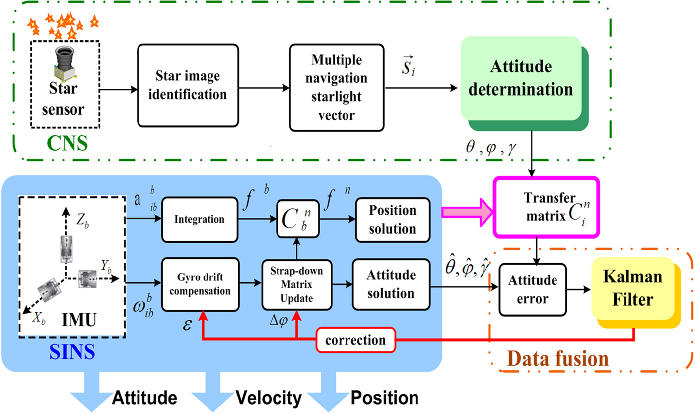
At present, most of the traditional SINS/CNS integrated navigation schemes are based on the gyro-drift-corrected mode, whose working principle is shown in Figure 1 (Hong et al., Reference Hong, Liu, Chen and Deng2010; He et al., Reference He, Wang and Fang2014).

Figure 1. Schematic diagram of a gyro-drift-corrected SINS/CNS integrated navigation scheme.

CNS can obtain attitude according to the navigation star vector's inertial frame, while SINS would provide the auxiliary matrix information $C_{i}^{n}$ to convert the attitude to the navigation frame. The differences of attitude between CNS and SINS are then sent to the filter for data fusion. Misalignment angles and gyroscope drifts can be estimated and corrected effectively. However, on one hand, the navigation errors of SINS have been introduced into the transfer matrix $C_{i}^{n}$ and on the other hand, due to the bias of the accelerometer, position errors will gradually accumulate and cannot be compensated. This results in a slow divergence in the navigation solution with time. Obviously, this kind of scheme cannot meet the requirements of long-endurance and high-accuracy navigation.

In order to improve the performance of the integrated navigation system mentioned above, a SINS/CNS integrated navigation scheme based on overall optimal correction is proposed for a HALE UAV. The integrated navigation scheme is composed of three parts: SINS subsystem, CNS subsystem and data fusion subsystem, as shown in Figure 2.

Figure 2. Schematic diagram of the proposed SINS/CNS integrated navigation scheme.

In the SINS subsystem, outputs of the IMU include angular rate $\omega_{lib}^{b}$ and specific force $f_{lib}^{b} \cdot \omega_{lib}^{b}$ and $f_{lib}^{b}$ are used to calculate the position $\hat{\lambda},\hat{L},\hat{h}$, velocity $\hat{v}$ and attitude $\hat{\theta},\hat{\varphi},\hat{\gamma}$ via the navigation solution mode. As the large FOV star sensor can observe multiple starlight vectors simultaneously, it is convenient to capture navigation stars and refraction stars. Navigation star vectors can be used to solve attitude $\theta,\varphi,\gamma$. Apparent height ${\tilde{h}}_a$, which is used to calculate position λ, L, h, can be acquired by refraction stars and a stellar refraction model. As the observing noise of ${\tilde{h}}_a$ cannot be neglected, a digital filter is introduced to pre-process the measurement ${\tilde{h}}_a$ to improve the accuracy of positioning. The CNS will also provide the horizontal reference $C^{n}_{i}$, which is important for attitude conversion. The Kalman filter is then used for data fusion and measurements of the Kalman filter include attitude difference φ and position difference δ_p (Zhang et al., Reference Zhang, Fu, Ge and Tang2014). Finally, misalignment angles $\Delta\varphi$, position errors $\delta_{\hat{{\rm p}}}$ and drifts of gyroscopes and bias of accelerometers can be estimated and corrected efficiently. Estimated states are then chosen to feed back so that the errors of SINS can be compensated efficiently (Quan et al., Reference Quan, Fang, Xu and Sheng2008).

Comparing the two schemes above, it is clear that the proposed integrated navigation system based on overall optimal correction has advantages as follows:

1. (1) CNS can provide comprehensive independent navigation information. For the traditional gyro-drift-corrected scheme, CNS can only provide attitude information, while in the proposed scheme, CNS can output attitude, position and horizon references independently.

2. (2) CNS is not constrained by the errors of SINS. In the traditional navigation scheme, star sensor measurement error, centroid extraction error and pattern matching error (Wang et al., Reference Wang, Zhou, Cheng and Lin2012) are introduced, and SINS error is also included. However, in the proposed scheme, regardless of attitude or position determination, CNS is free from the influence of SINS errors. The reduction error sources can effectively slow down the divergence trend, which is more suitable for long-endurance navigation.

3. (3) The errors of SINS can be estimated and corrected more comprehensively. In the traditional scheme, only misalignment angles and the gyro constant drifts can be estimated. In the proposed method, excepting misalignment angles and gyro drifts, position and velocity errors and accelerometer bias can be effectively estimated and compensated. Consequently, the navigation accuracy of the proposed scheme has been greatly improved.

2.2. Installation angle design

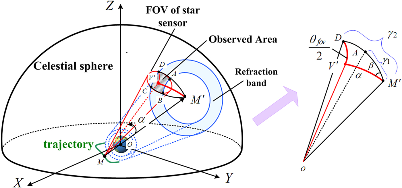
The large FOV star sensor is required to observe two kinds of starlight: one is navigation starlight, which is used for attitude determination and the other is refraction starlight, which is essential for calculating position. Obviously, installation angle and direction of optical axis are important factors, which will affect the observation results and then affect the accuracy of attitude and position. Therefore, it is necessary to find a reasonable installation angle.

As shown in Figure 3, the refraction area consists of two blue dotted circles and the two black dotted lines are the boundary of the FOV. Installation angle α is the included angle between the negative direction of position vector $-\vec{r}_{s}$ and the optical axis direction vector $\vec{V}_{b}$. Generally, it is better to make the optical axis $\vec{V}_{b}$ point to the refraction area, so that refraction stars can fall within the scope of the FOV to the greatest degree. By taking all the factors that may affect the accuracy of the atmospheric refraction model into consideration, we choose refracted height h _g ranging from h _g1=20 km to $h_{g2} = 25\,\hbox{km}$ (Yang et al., Reference Yang, Yang, Zhu and Li2015). The critical refracted starlight ${\mathop{S}\limits^{\rightharpoonup}}_{1}$ and ${\mathop{S}\limits^{\rightharpoonup}}_{2}$, at the height of h _g1, h _g2, are shown in Figure 3. The critical refraction angles R ₁ and R ₂ will be acquired by the empirical formula:

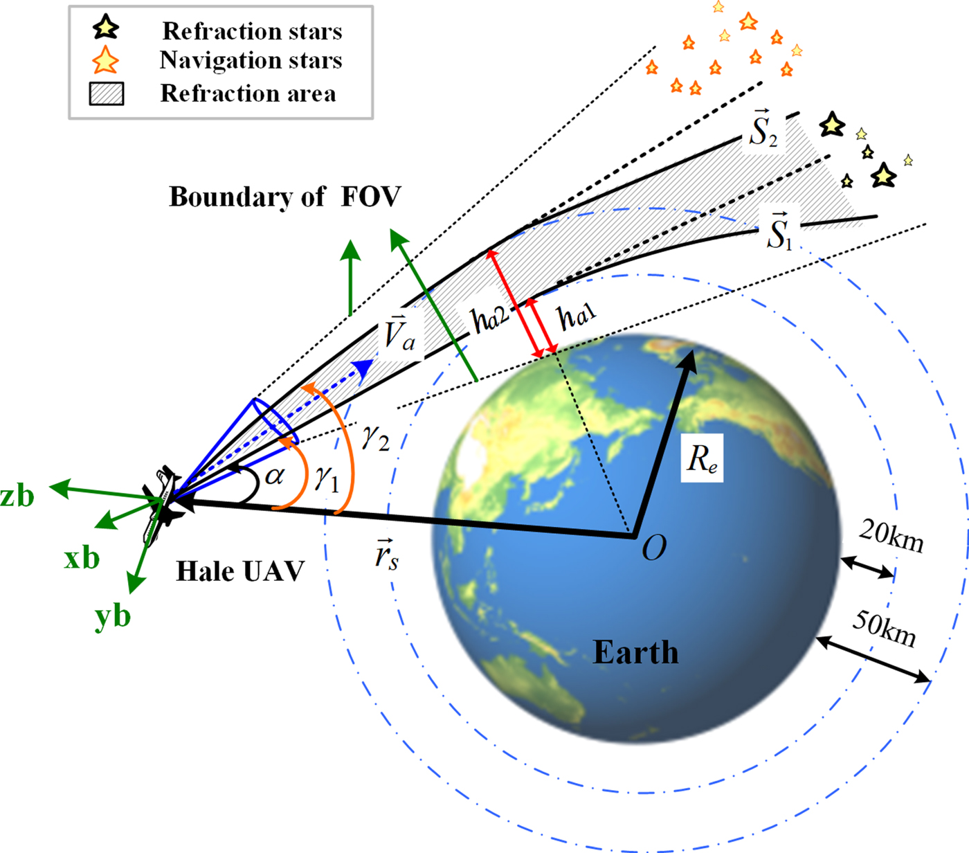
Figure 3. Diagrammatic sketch of the installation angle.

(1)$$\lcub \eqalign{& R_{1}=6965{\cdot}4793\ e^{-0{\cdot}15180263\ h_{g1}}\cr & R_{2}=6965{\cdot}4793\ e^{-0{\cdot}15180263\ h_{g2}}} $$

Angle γ is defined as the included angle between position vector ${\mathop{r}\limits^{\rightharpoonup}}_{\!s}$ and refracted starlight vector ${\mathop{S}\limits^{\rightharpoonup}}$ and it can be calculated by the following formula:

(2)$$\gamma = \arccos \left({\mathop{r}\limits^{\rightharpoonup}}_{\!s}\cdot \vec{S}\over{|{\mathop{r}\limits^{\rightharpoonup}}_{\!s}|}\right)$$

where $r_{s}=|{\mathop{r}\limits^{\rightharpoonup}}_{\!s}|$ is the geocentric distance and R _e is the Earth's radius.

According to Equation (1), the value range of γ can be acquired as follows:

(3)$$\left\{\eqalign{& \gamma_{1}\leq\gamma \leq\gamma_{2} \cr & \gamma_{1}= \arcsin \left({R_{e}+h_{a1}\over r_{s}}\right) \cr & \gamma_{2}= \arcsin \left({R_{e}+h_{a2}\over r_{s}}\right)}\right.$$

The direction of the star sensor's optical axis $\vec{V}_{b}$ can be adjusted by installation angle α. If $\vec{V}_{b}$ is located in the shadow area formed by critical refracted starlight ${\mathop{S}\limits^{\rightharpoonup}}_{\!1}$ and ${\mathop{S}\limits^{\rightharpoonup}}_{\!2}$, there are a large number of refraction stars which can be captured by the star sensor. Therefore, it is necessary to find a reasonable installation angle α.

Figure 4 illustrates the geometric relationship of Figure 3 when projected onto the celestial sphere. Once the position of the HALE UAV M is acquired, its projection M′ is as shown in Figure 4. If the refraction area 20 km–50 km is projected onto the celestial sphere, it would generate an annular area on the surface of the sphere, just as the blue annular shown in Figure 4. The red circle is the projection of the star sensor's FOV and optical axis vector $\mathop{V}\limits^{\rightharpoonup}$ intersecting with the spherical surface at point V′ which is the centre point of the red circle. The red circle has an overlapping part with a blue annular area, just as the hatched region ABCD shown in Figure 4. Stars located in this area are refraction stars which can be observed by the star sensor. Since the area of ABCD is decided by installation angle α, when the area value S _ABCD reaches its maximum, installation angle α is optimal for observing refraction stars. However, the value of S _ABCD can be reflected by included angle β between $D\!\mathop{M}\limits^{\cap}{}^{\prime}$ and $V'\!\!\mathop{M}\limits^{\cap}{}^{\prime}$. Obviously, when the angle β achieves its maxmuim, installation angle α is correspondingly optimal.

Figure 4. Geometric sketch of the installation angle in the celestial sphere.

As shown in Figure 4, $A\!\mathop{M}\limits^{\cap}{}^{\prime}$ and $D\!\mathop{M}\limits^{\cap}{}^{\prime}$ are both large arcs. According to the definition of the blue annulus, $A\!\mathop{M}\limits^{\cap}{}^{\prime}=\gamma_{1}$ and $D\!\mathop{M}\limits^{\cap}{}^{\prime}=\gamma_{2}$. Since $D\!\mathop{V}\limits^{\cap}{}^{\prime}$ is the radius of the red circle, the angular distance is $\theta_{fov}/2$. In the spherical triangle M′DV′, according to the cosine law of a spherical triangle, the following equation is formulated:

(4)$$\cos{\theta_{fov}\over 2}=\cos\, a\, \cos\gamma_{2}+\sin\alpha \sin\gamma_{2}\cos\beta$$

where $\theta_{fov}$ is the FOV of the star sensor, α is the installation angle and β is the included angle between $D\!\mathop{M}\limits^{\cap}{}^{\prime}$ and $ V'\!\mathop{M}\limits^{\cap}{}^{\prime}$. Then angle β can be determined:

(5)$$\beta=\arccos \left\{\cos {\theta_{fov}\over 2}-\cos\alpha\cos\gamma_{2}\over \sin\alpha\sin\gamma_{2}\right\}$$

The differential of Equation (5) is written as:

(6)$$\beta^\prime={\left(\cos{\theta_{fov}\over 2}\cos\alpha-\cos\gamma_{2}\right)\sin\gamma_{2}\over(\sin\alpha\sin\gamma_{2})^{2} \sqrt{1-\left({\cos{\theta_{fov}\over 2}-\cos\alpha\cos\gamma_{2}\over \sin\alpha\sin\gamma_{2}}\right)^{2}}}$$

When β′=0, the value of α is:

(7)$$\alpha = \arccos \left(\cos\gamma_{2}\over{\cos{\theta_{fov}\over 2}}\right)$$

From Equations (3) and (7), it can be summarised that the optimal installation angle is decided by the FOV of the star senor $\theta_{fov}$, refracted height h _g and position of the HALE UAV $\vec{r}_{s}$.

It is clear that, when the star sensor and refracted height are selected, $\theta_{fov}$ and h _g are constants. So, the installation angle α varies with position information $\vec{r}_{s}$. However, the installation angle of the star sensor cannot be changed. In order to make it possible to point the optical axis to the designated area, an attitude manoeuvre method is introduced. When a HALE UAV is flying for a long time, the navigation computer can provide navigation parameters and calculate attitude control commands in real time. Then the UAV will rotate around the centre of mass according to the attitude control commands to ensure the optical axis points to the best area. In addition, this ensures that there are enough refracted stars captured in the FOV of the star sensor.

3.1. Position and horizontal reference determination algorithm

The density of the atmosphere is uneven. Consequently, when starlight passes through the atmosphere, it will be refracted and then bend gradually towards the centre of the Earth. Therefore, viewed from a HALE UAV, the position of an apparent star will be higher than that of the actual star. Apparent ray $\vec{u}_{a}$ diverges from actual ray $\vec{u}_{s}$ as shown in Figure 5. Angle R between $\vec{u}_{a}$ and $\vec{u}_{s}$ is defined as the refraction angle. According to Figure 5, the refracted ray appears to graze the horizon of the Earth at an apparent height h _a, but is actually at a slightly lower height h _g. There is a nonlinear mathematical relation between apparent height h _a and position vector $\vec{r}_{s}$.

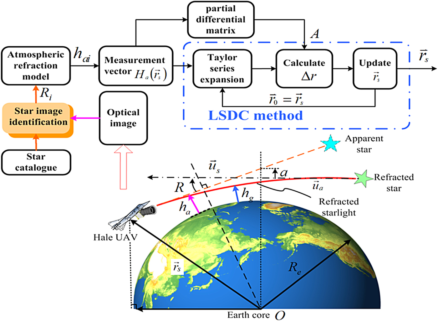
Figure 5. Schematic diagram of position determination algorithm.

In order to acquire position information, it is necessary to solve nonlinear equations. The Least Square Differential Correction (LSDC) method, which is efficient in dealing with the nonlinear measurement, is introduced in this paper. Figure 5 illustrates the process of position determination based on LSDC. It includes the following six steps:

Step 1. Acquire refraction angle R. Firstly, it is necessary to obtain the refraction angle R. After star image identification (Wang et al., Reference Wang, Wang and Li2012), the position of a refraction star in measuring frame (s) can be denoted as $\mathop{S}\limits^{\rightharpoonup}{\!}_{rs}$:

(8)$$\mathop{S}\limits^{\rightharpoonup}{\!}_{rs}={1\over \sqrt{(x_{r}-x_{0})^{2}+(y_{r}-y_{0})^{2}+f^{2}}}\left[\matrix{-(x_{r}-x_{0})\cr -(y_{r} -y_{0})\cr f }\right]$$

where (x _r, y _r) is the centre point of this refraction star in the (s) frame, (x ₀, y ₀) is the centre point of the lens in the (s) frame and f is the focal length of the star sensor.

The actual position of the star in the (i) frame is $\vec{S}_{i}$, which can be obtained by reference to a star catalogue after star image identification. Then, combined with installation matrix $C_{s}^{b}$ and attitude matrix $C^{b}_{i}$, vector $\vec{S}_{i}$ can be transformed into the (s) frame as Equation (9) shows:

(9)$$\vec{S}_{iS}=(C_{s}^{b})^{T}C_{i}^{b}\vec{S}_{i}$$

Therefore, based on the definition of refraction angle R, R can be determined by the following equation:

(10)$$R= \arccos\lpar \lpar \vec{S}_{rs}\rpar^{T}\vec{S}_{is}\rpar $$

Step 2. Construct measurement matrix H _a. There is an accurate function describing the relationship between refraction angle R and refraction height h _g (Yang et al., Reference Yang, Si, Xu and Zhou2014):

(11)$$h_{g}=h_{0}-H\ln(R)+H\ln(\rho_{0})+H\ln\left(k(\lambda)\sqrt{{2\pi R_{e}\over{H}}}\right)$$

where h ₀ is a reference height; k(λ) is the scattering coefficient; R _e is Earth's radius; ρ₀ is the atmospheric density at height of h ₀ and H is the atmospheric density scale height.

Assuming that the atmosphere satisfies spherical lamination, according to the optical refraction law, refraction height h _g and apparent height h _a have the following relationship:

(12)$$h_{a}=h_{g}+(R_{e}+h_{g})\cdot \sqrt{H\over 2\pi R_{e}}$$

Associating Equation (11) with Equation (12) and taking R _e≫h _a into consideration, it is easy to deduce the mathematical formula between h _a and R:

(13)$$h_{a}=h_{0}-H\ln(R)+H\ln(\rho_{0})+H\ln\left(k(\lambda)\sqrt{2\pi R_{e}\over{H}}\right)+R\sqrt{HR_{e}\over{2\pi}}$$

where $H,\rho_{0},h_{0}, R_{e},k(\lambda)$ are all constant when λ is given. Once a refraction angle is acquired, corresponding height h _a is also derived via Equation (13).

As is shown in Figure 5, apparent height h _a, refraction angle R, and the UAV's geocentric distance r _s satisfy the following equation:

(14)$$h_{a}=\sqrt{{\mathop{r_{s}}\limits^{\rightharpoonup}{\!}}^2 - u^{2}}+u\tan(R)-R_e-a$$

where $\vec{r}_{s}$ is the position vector and $\vec{u}_{s}=[\cos\ \delta_{s}\ \cos\ \alpha_{{\rm s}},\ \cos\ \delta_{s}\ \sin\ \alpha_{s},\ \sin\ \delta_{S}]^{T}$ is the unit position vector of the refraction star in the (i) frame. δ_s is declination and α_s is right ascension. $u=|\vec{r}_{s}\cdot\vec{u}_{s}|$ and a is a small constant as shown in Figure 5 and is usually neglected when calculating h _a. When starlight is close to the surface of the Earth, the refraction will become more obvious. So, refraction of starlight mainly occurs in the stratosphere and troposphere. Refracted starlight observed from the top of the stratosphere is little different to that observed from outside the atmosphere (Hays and Roble, Reference Hays and Roble1967). According to Equations (13) and (14), the positioning error caused by the refraction angle is about 134·93 m when the measuring error of the star sensor is 3$^{\prime\prime}$ and its height is 30 km. Therefore, if the accuracy of the star sensor is high enough, the influence of the refraction angle on positioning accuracy can be controlled in a very small range. So, as long as a HALE UAV is flying beyond the stratosphere (more than 30 km), the traditional star refraction model is still available.

We assume that there are n (n≥3) refraction stars which are captured by the star sensor. According to Equation (7), refraction angles $[R_{1},R_{2}\ldots R_{n}]^{T}$ can be acquired. Based on Equation (14), measurement vector $H_{a}({\mathop{r}\limits^{\rightharpoonup}}_{\!s})$ is also acquired:

(15)$$H_{a}(\mathop{r_{s}}\limits^{\rightharpoonup})=\left[\matrix{h_{a1}\cr h_{a2}\cr \vdots \cr h_{an}}\right] = \left[\matrix{\sqrt{\vec{r}_{s}^{2}-u_{1}^{2}}+u_{1}\tan(R_{1})-R_{e}\cr \sqrt{\vec{r}_{s}^{2}-u_{2}^{2}}+u_{2}\tan(R_{2})-R_{e}\cr \vdots\cr \sqrt{{\mathop{r_{s}}\limits^{\rightharpoonup}}^{2}-u_{n}^{2}}+u_{n}\tan(R_{n})-R_{e}}\right]$$

where h _ai is the apparent height of the ith refraction star; $\vec{r}_{s}=[r_{x}\ r_{y}\ r_{z}]^{T}$ isthe position vector of the HALE UAV; $\vec{u}_{Si}=[\cos\ \delta_{Si}\ \cos\ \alpha_{Si},\ \cos\ \delta_{Si}\ \sin\ \alpha_{Si},\ \sin\ \delta_{Si}]^{T}$ is the unit position vector of the i-th star in the (i) frame and $u_{i}=|\vec{r}_{s}\cdot \mathop{u}\limits^{\rightharpoonup}{\!}_{Si}|(i=(1,2,\ldots n))$. Equation (15) is an equation with three unknown quantities r _x, r _y, r _z.

Step 3. Solve position $\vec{r}_{s}$ based on measurement vector H _a. We choose $\vec{r}_{s0}$ as the initial value of position vector ${\mathop{r}\limits^{\rightharpoonup}}_{\!s}$ and the first-order Taylor series expansion of Equation (15) at the point of $\vec{r}_{s0}$ is expressed as:

(16)$$H_{a}(\mathop{r}\limits^{\rightharpoonup}{\!}_{s})=H_{a}(\mathop{r}\limits^{\rightharpoonup}{\!}_{s0})+A\cdot \Delta\mathop{r}\limits^{\rightharpoonup}{\!}+V$$

where V is the residual sequence of the first order Taylor expansion of Equation (16); $\Delta{\mathop{r}\limits^{\rightharpoonup}}=\vec{r}_{s}-\vec{r}_{s0}$ is the differential correction and A is the partial derivative matrix of $H_{a}(\vec{r}_{s})$ with respect to the position vector $\mathop{r}\limits^{\rightharpoonup}{\!}_{s}$. It can be calculated by the following formula:

(17)$$A=\displaystyle{\partial H_{a}(r_{s})\over \partial r_{s}}=\left[\matrix{\displaystyle{\partial h_{a1}\over r_{x}} & \displaystyle{\partial h_{a1}\over r_{y}} & \displaystyle{\partial h_{a1}\over r_{z}}\cr \displaystyle{\partial h_{a2}\over r_{x}} & \displaystyle{\partial h_{a2}\over r_{y}} & \displaystyle{\partial h_{a2}\over r_{z}}\cr \vdots & \vdots & \vdots\cr \displaystyle {\partial h_{an}\over r_{x}} & \displaystyle{\partial h_{an}\over r_{y}} & \displaystyle{\partial h_{an}\over r_{z}}}\right]$$

(18)$$\left\{\eqalign{& \displaystyle{\partial ha_i\over r_x} = \displaystyle{r_x-u_i\cdot \cos \delta_i \cos\alpha_i\over \sqrt{r^2_s-u_i^2}}\cr & \displaystyle{\partial ha_i\over r_y} = \displaystyle{r_y-u_i\cdot \cos \delta_i \sin\alpha_i \over \sqrt{r^2_s-u_i^2}}\quad{(i =1,2,\ldots n)}\cr & \displaystyle{\partial ha_i\over r_z} = \displaystyle{r_z-u_i\cdot \sin\delta_i\over \sqrt{r^2_s-u_i^2}}}\right.$$

Then the value of differential correction $\Delta\hat{r}$ can be acquired from the following equation:

(19)$$\Delta\hat{r}=(A^{T}A)^{-1}A^{T}(H_{a}(\mathop{r}\limits^{\rightharpoonup}{\!}_{s})-H_{a}(\vec{r}_{s0}))$$

Updated $\mathop{r}\limits^{\rightharpoonup}{\!}_{s}$ with $\Delta\hat{r}$:

(20)$$\vec{r}_{sc}=\vec{r}_{s0}+\Delta r$$

The process above is repeated by using the corrected $\vec{r}_{sc}$ as the initial value $\vec{r}_{s0}$ in the next turn until the difference between $\vec{r}_{sc}$ and $\vec{r}_{s0}$ satisfies the iteration termination requirement $|\mathop{r}\limits^{\rightharpoonup}{\!}_{sc}-\mathop{r}\limits^{\rightharpoonup}{\!}_{s0}|<\varepsilon$. The solution of $\mathop{r}\limits^{\rightharpoonup}{\!}_{s}$ is $\vec{r}_{s0}$.

Since position vector $\mathop{r}\limits^{\rightharpoonup}{\!}_{s}=[r_{x}\ r_{y}\ r_{z}]^{T}$ has been solved, it is convenient to calculate declination δ_d, right ascension α_d and height h of a HALE UAV in the (i) frame:

(21)$$\eqalign{&\alpha_{d}=\arctan(r_{y}/r_{x})\cr & \delta_{d}=\arctan\!\left(r_{z}/\sqrt{r_{x}^{2}+r_{y}^{2}}\right)\cr & h=r_{z}-R_{e}}$$

where $\alpha_{d}\in (0\sim 2\pi)$, $\delta_{d}\in (-\pi/2\sim \pi/2)$. Then, declination δ_d and right ascension α_d can be transformed to the navigation frame (n). Therefore, geographic latitude L and longitude λ can be written as:

(22)$$\eqalign{&\lambda =\alpha_{d}-t_{G} \cr & L=\delta_{d}}$$

where t _G is the Greenwich Hour Angle (GHA) of the Spring Equinox.

Step 4. Extract horizontal reference. Position vector $\mathop{r}\limits^{\rightharpoonup}{\!}_{s}$ obtained in Step 3 can also be used to calculate matrix $C^{n}_{i}$ since $\mathop{r}\limits^{\rightharpoonup}{\!}_{s}$ contains the horizontal information. $\vec{p}$ represents the unit position vector which can be expressed as:

(23)$$\vec{p}=\mathop{r}\limits^{\rightharpoonup}{\!}_{s}/|\mathop{r}\limits^{\rightharpoonup}{\!}_{s}|=[p_{x}\ p_{y}\ p_{z}]^{T}$$

Matrix $C^{n}_{i}$ can be derived by the following formula:

(24)$$C_{i}^{n}=\left[ \matrix{-\displaystyle{p_{y}\over \sqrt{1-p_{z}^{2}}}, & \displaystyle{p_{x}\over \sqrt{1-p_{z}^{2}}} & 0 \cr -\displaystyle{p_{x}p_{z}\over \sqrt{1-p_{z}^{2}}} & -\displaystyle{p_{y}p_{z}\over \sqrt{1-p_{z}^{2}}} & \sqrt{1-p_{z}^{2}}\cr p_x & p_y & p_{z}} \right]^{T}$$

Up to now, position and horizontal references with high-accuracy have both been acquired via the least square differential correction method.

3.2. Attitude determination algorithm

Assuming that n (n>3), navigation stars can be captured, and will generate an optical image on the Charge Coupled Device (CCD) surface. $(x_{Si},\ y_{Si})$ is the centre point of the i-th navigation star in (s) frame. The i-th starlight vector can be formulated as:

(25)$$S_{is}={1\over \sqrt{x_{si}^{2}+y_{si}^{2}+f^{2}}}\left[\matrix{ x_{Si}\cr y_{Si}\cr -f }\right],\ (i=1,2\cdots n)$$

where f is the focal length of the star sensor.

Multiple vectors of n (n>3) stars in (s) frame are denoted as C _s. Position vectors of n stars C _i, in the (i) frame can be acquired by star image identification. According to the installation relationship between a star sensor and a HALE UAV, it is easy to calculate the installation matrix $M_{s}^{b}$. Then the attitude matrix $A_{b}^{i}$ has the following relationship with C _s, C _i, and $M_{s}^{b}$:

(26)$$c_i =A_{b}^i M_{s}^{b}C_{s}$$

Finally, the high precision attitude matrix $A^{i}_{b}$ can be calculated by using the least squares method.

Equation (24) provides horizontal reference $C^{n}_{i}$ and combined with $A^{i}_{b}$ solved in Equation (26), it is easy to acquire matrix $C_{b}^{n}$ which can be used to calculate attitude information:

(27)$$C_{b}^{n}=C^{n}_i\cdot A_{b}^i$$

According to the definition of attitude angles, $[\varphi,\ \gamma,\psi]^{T}$ are derived by the following formula:

(28)$$\left[\matrix{ \varphi\cr \gamma\cr \psi}\right]=\left[ \matrix{ \arcsin\!C_{b}^{n}(3,2)\cr -\arctan[C_{b}^{n}(3,1)/C_{b}^{n}(3,3)]\cr \arctan[C_{b}^{n}(1,2)/C_{b}^{n}(2,2)] }\right]$$

Based on the analysis above, it is summarised that the proposed SINS/CNS scheme relying on a single large FOV star sensor is able to provide real-time position, horizontal reference and attitude information for a HALE UAV. The positioning algorithm principle of a star sensor is simple with only a small amount of calculation. The horizontal reference is totally free from SINS, which results in a higher attitude precision.

4.1. System model

We select the misalignment angles, velocity errors, position errors, drifts of gyroscopes and zero biases of accelerometers as system states. According to error equations of SINS, the system model is as below:

(29)$$\dot{X}=FX+CW$$

where the state vector is $X=[\phi_{x},\ \phi_{y},\ \phi_{z},\ \delta v_{x},\ \delta v_{y},\ \delta v_{z},\ \delta L,\ \delta\lambda,\ \delta h,\ \varepsilon_{x},\ \varepsilon_{y},\ \varepsilon_{z},\ \nabla_{x},\ \nabla_{y},\ \nabla_{z}]^{T}$, including misalignment angles $\phi_{x},\phi_{y},\phi_{z}$, velocity errors $\delta v_{x},\delta v_{y},\delta v_{z}$, position errors $\delta L,\ \delta\lambda,\delta h$, gyroscope drifts $\varepsilon_{x},\varepsilon_{y},\varepsilon_{z}$ and accelerometers biases $\nabla_{x},\ \nabla_{y},\ \nabla_{z}$.

F is the state transition matrix:

(30)$$F=\left[\matrix{ F_{N(9\times 9)} & F_{S(6\times 6)}\cr 0_{(6\times 9)} & 0_{(9\times 6)}} \right]$$

Non-zero elements of F _N are:

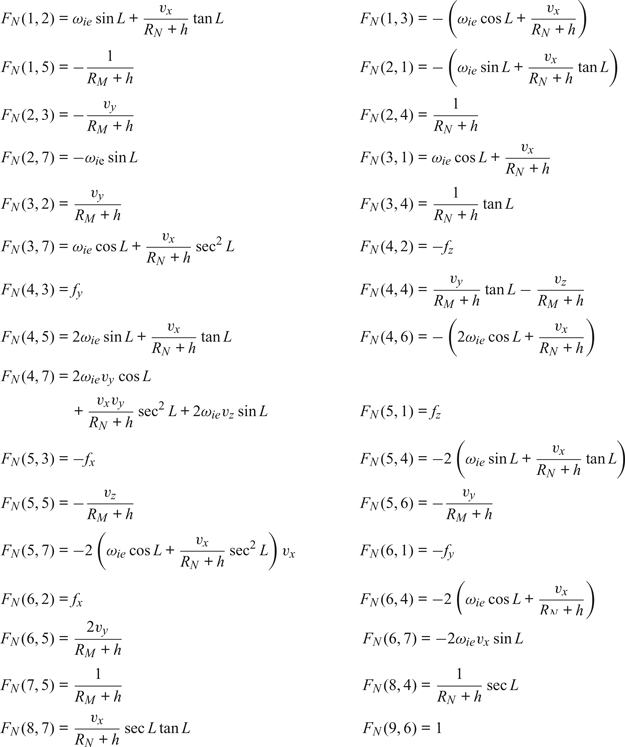
where ω_ie is the rotational angular velocity of the Earth; v _x, v _y, v _z is the velocity provided by SINS; f _x, f _y, f _z is the specific force along the three axes; R _M is the main radius of curvature of the meridian and R _N is the main radius of curvature of prime vertical.

F _s can be expressed as:

(31)$$F_{S}=\left[\matrix{ -C_{b}^{n} & 0_{3\times 3}\cr 0_{3\times 3} & C_{b}^{n} }\right]$$

G is the noise driven array:

(32)$$G=\left[\matrix{ -C_{b}^{n} & 0_{3\times 3}\cr 0_{3\times 3} & C_{b}^{n}\cr 0_{9\times 3} & 0_{9\times 3}}\right]$$

$W=[\omega_{gx}\ \omega_{gy}\ \omega_{gz}\ \omega_{dx}\ \omega_{dy}\ \omega_{dz}]^{T}$ is the noise vector, where $\omega_{gx},\omega_{gy},\omega_{gz}$ is the noise of the gyroscope and $\omega_{dx},\omega_{dy},\omega_{dz}$ is the noise of the accelerometer along the three axes.

4.2. Measurement model

Misalignment angles and position errors are selected to be measurements of Kalman filter. The misalignment angle vector can be calculated from the attitude error of SINS and CNS. $\delta =[\delta\theta,\ \delta\varphi,\ \delta\gamma]$ stands for attitude error and according to its definition, it can be expressed as:

(33)$$\lcub \eqalign{&\delta\theta=\hat{\theta}-\theta\cr & \delta\varphi=\hat{\varphi}-\varphi\cr & \delta\gamma=\hat{\gamma}-\gamma} $$

where $\hat{\theta},\hat{\varphi},\hat{\gamma}$ is the attitude of SINS and $\theta,\varphi,\gamma $ is the attitude provided by CNS.

Assuming that $\hat{C}_{n}^{b}$ is the attitude matrix calculated by SINS and the actual attitude matrix is $C_{n}^{b}$, these two matrices satisfy the following equation:

(34)$$C_{n}^{b}=\hat{C}_{n}^{b}C_{n}^{p}=\left[\matrix{ C_{11} & C_{12} & C_{13}\cr C_{21} & C_{22} & C_{23}\cr C_{31} & C_{32} & C_{33} }\right] = \left[\matrix{ \hat{C}_{11} & \hat{C}_{12} & \hat{C}_{13}\cr \hat{C}_{21} & \hat{C}_{22} & \hat{C}_{23}\cr \hat{C}_{31} & \hat{C}_{32} & \hat{C}_{33} }\right] \left[\matrix{ 1 &\phi_{z} &-\phi_{y}\cr -\phi_{z} &1 &\phi_{x}\cr \phi_{y} &-\phi_{x} & 1 }\right]$$

According to the identification of $C_{n}^{b}$, it is clear that $\sin\theta=C_{23}$, $\tan\varphi =C_{21}/C_{22}$ and $\tan\gamma=-C_{13}/C_{33}$. Referring to Equations (33) and (34), the following three equations are given as:

(35)$$\sin(\hat{\theta}-\delta\theta)=-\phi_{y}\hat{C}_{21}+\phi_{x}\hat{C}_{22}+\hat{C}_{23}$$

(36)$$\tan(\hat{\varphi}-\delta\varphi)={\hat{C}_{21}-\phi_{z}\hat{C}_{22}+\phi_{y}\hat{C}_{23}\over \phi_{z}\hat{C}_{21}+\hat{C}_{22}-\phi_{x}\hat{C}_{23}}$$

(37)$$\tan(\hat{\gamma}-\delta\gamma)=-{-\phi_{y}\hat{C}_{11}+\phi_{x}\hat{C}_{12}+\hat{C}_{13}\over -\phi_{y}\hat{C}_{31}+\phi_{x}\hat{C}_{32}+\hat{C}_{33}}$$

We linearize the left parts of Equations (35), (36) and (37) and expand the right parts of Equation (35), (36) and (37) using the Taylor series. Equations (35), (36) and (37) can be transformed as the following three equations, when neglecting the second-order or more than second-order small quantity:

(38)$$\delta\theta =-\phi_{x}\cos\hat{\varphi}+\phi_{y}\sin\hat{\varphi}$$

(39)$$\delta\varphi =-\phi_{x}\sin\hat{\varphi}\tan\hat{\theta}-\phi_{y}\cos\hat{\varphi}\tan\hat{\theta}+\phi_{z}$$

(40)$$\delta\gamma =-\phi_{x}{\sin\hat{\varphi}\over \cos\hat{\theta}}-\phi_{y}{\cos\hat{\varphi}\over \cos\hat{\theta}}$$

Therefore, the misalignment angles $\phi_{x},\phi_{y},\phi_{z}$ can be determined by attitude error:

(41)$$\left[\matrix{ \phi_{x}\cr \phi_{y}\cr \phi_{z} }\right]= \left[\matrix{ -\cos\hat{\varphi} &0 &-\sin\hat{\varphi} \cos\hat{\theta}\cr \sin\hat{\varphi} &0 &-\cos\hat{\varphi} \cos\hat{\theta}\cr 0 & 1 & -\sin\hat{\theta} }\right]\left[\matrix{ \delta\theta\cr \delta\varphi\cr \delta\gamma }\right]$$

Then the measurement equation can be expressed as:

(42)$$Z_{1}=H_{1}X+V_{1}$$

where $Z_{1}=[\phi_{x}\ \phi_{y}\ \phi_{z}]^{T}$; $H_{1}=[I_{3\times 3}\ 0_{3\times 12}]$ is the measuring vector and V ₁ stands for measuring noise.

When the measurement is the position error between SINS and CNS, the measurement equation can be expressed as:

(43)$$Z_{2}=H_{2}X+V_{2}$$

where $Z_{2}=[\hat{L}-L\ \hat{\lambda}-\lambda]^{T}$ is the position error; $\hat{L},\hat{\lambda}$ and L, λ are the position results provided by SINS and CNS; $H_{2}=[0_{2\times 6}\quad I_{2\times 2}\quad 0_{2\times 7}]$ is the corresponding measurement vector and V ₂ is measuring noise.

Therefore, based on Equations (42) and (43), the measurement model of SINS/CNS integrated navigation system is deduced as:

(44)$$Z=HX+V$$

where $Z=[Z_{1}\quad Z_{2}]^{T}$; $H=[H_{1}\quad H_{2}]^{T};V=[V_{1}\quad V_{2}]^{T}$.

Finally, the state model Equation (29) and the measurement model Equation (44) are linear, and a Kalman filter is utilised to estimate the state to correct the errors of SINS.

5.1. Simulation conditions

The simulation conditions are as follows (Wu et al., Reference Wu, Yu and Fang2006). Table 1 shows the initial navigation parameters and Table 2 gives the bias, drifts and noise of the related measuring devices. Table 3 sets the simulation time.

Table 1. Initial navigation parameters.

Table 2. Bias, drift and noise of measuring devices.

Table 3. Simulation time.

Based on the simulation conditions above, a UAV flight simulation scenario of four hours was designed and is illustrated in Figure 6. It includes all the motion pattems of the UAV, such as straight-line motion, turning motion, acceleration, deceleration, climbing and descending.

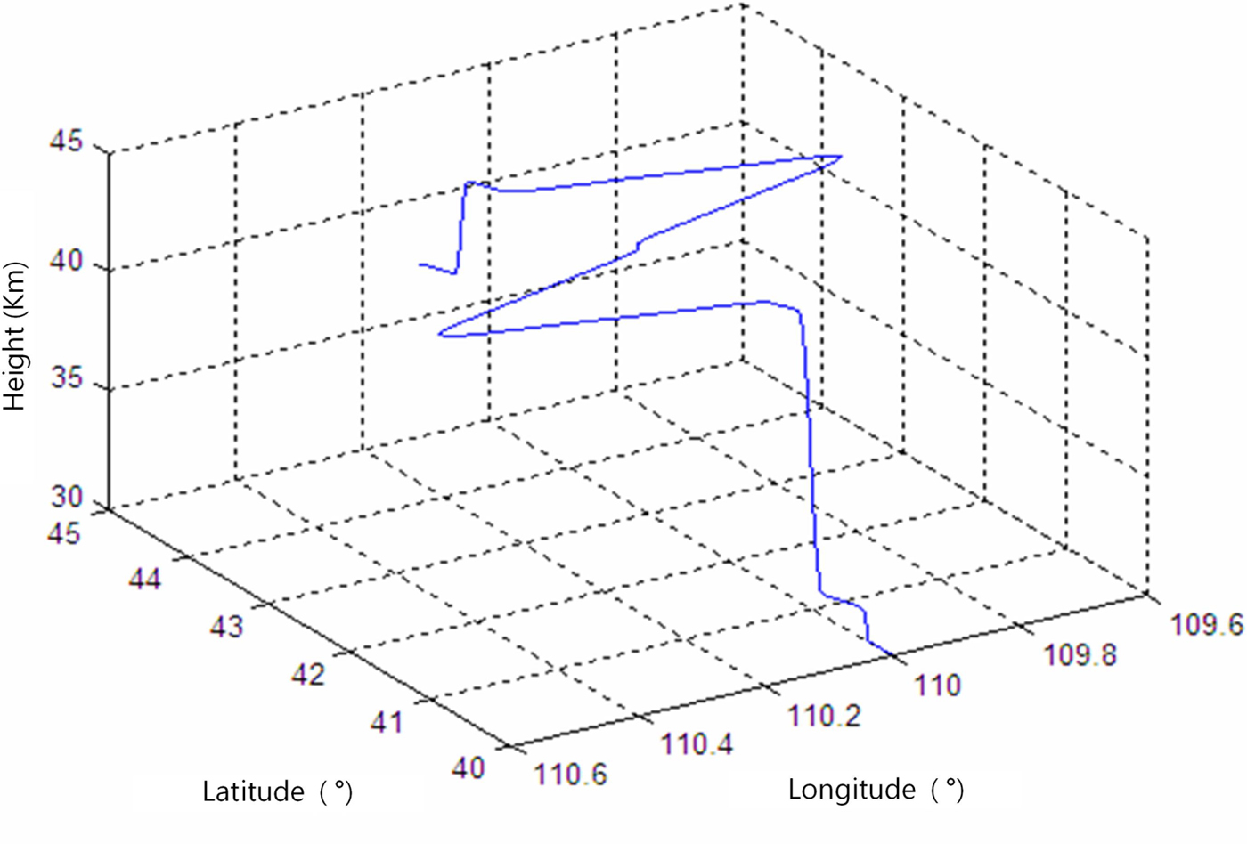
Figure 6. Simulated four hour HALE UAV trajectory.

5.2. Simulation results and analysis

5.2.1. Number of visible navigation and refraction stars

It is necessary to analyse the number of stars when a HALE UAV is flying for a long time. First, we exclude binary stars, variable stars and the stars whose magnitude is greater than 6·5 in the Tycho2 catalogue (Høg et al., Reference Høg, Fabricius, Makarov, Urban, Corbin and Wycoff2000), and a simplified whole-sky star catalogue can be determined. The FOV of the star sensor is $20^{\circ}\times 20^{\circ}$, and the resolution of the image plane is defined as $\hbox{Nx} \times \hbox{Ny}=1024\times 1024$. Pixel size is 14·7 μm. The total observing time is one hour, and the interval time is set as 1 s. The number navigation stars and refraction stars screened by the star sensor in one hour is shown in Table 4. N _n stands for the number of navigation stars and N _r stands for the number of refraction stars.

Table 4. Statistical table of number of stars screened by star sensor in one hour.

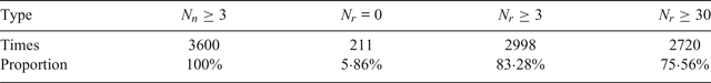
It can be seen clearly from Table 4, that over the whole hour, there are always more than three navigation stars in the FOV of the star sensor. This means that the attitude determination procedure can be carried out successfully. On only a few occasions (5·86% of total time) does the star sensor fail to capture refraction stars. However, during 83·28% of the whole period, the number of refraction stars is more than three. So, we contend that the proposed pure analytic positioning algorithm based on stellar refraction is feasible.

5.3. System performance verification and analysis

Based on the information above, the performance of the analytical positioning method is verified. We select the variance of refracted height noise as 80 m when there are more than three refraction stars, and the CNS can update the position of the UAV. While there are less than three refraction stars, CNS uses the positioning results at the last good fix. Simulation positioning results are shown in Figure 7. Results show that the proposed pure celestial analytic positioning algorithm is feasible. When the HALE UAV is flying for one hour, latitude error is maintained at about 500 m and longitude error does not exceed 1,000 m. The maximum height error is less than 60 m.

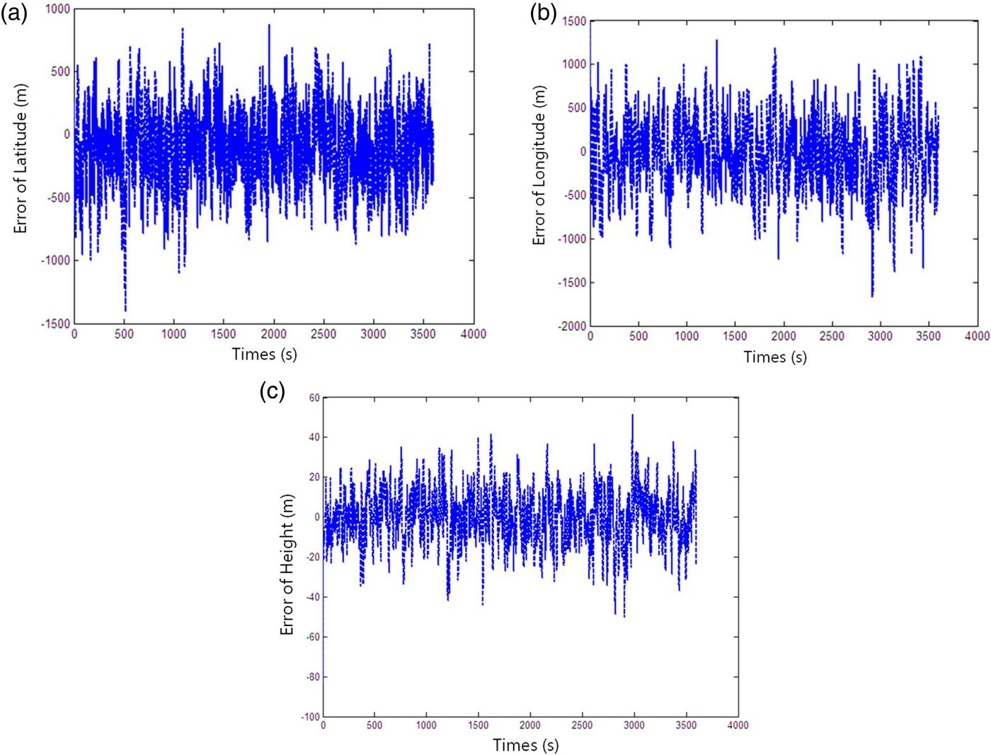
Figure 7. Position error of pure celestial analytic position algorithm.

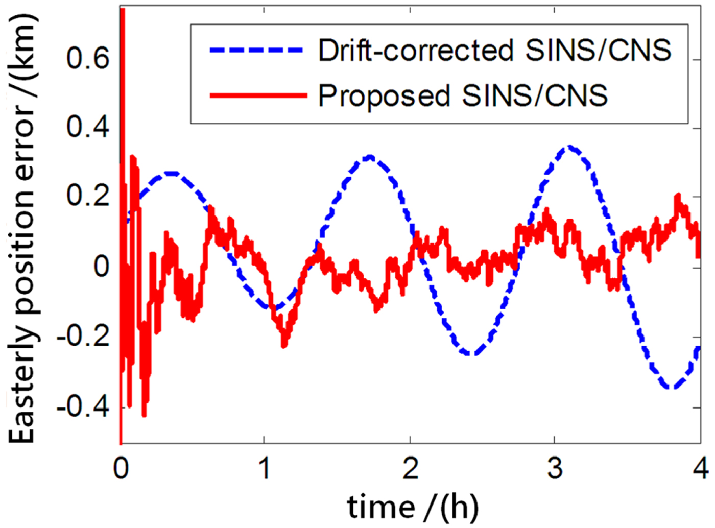
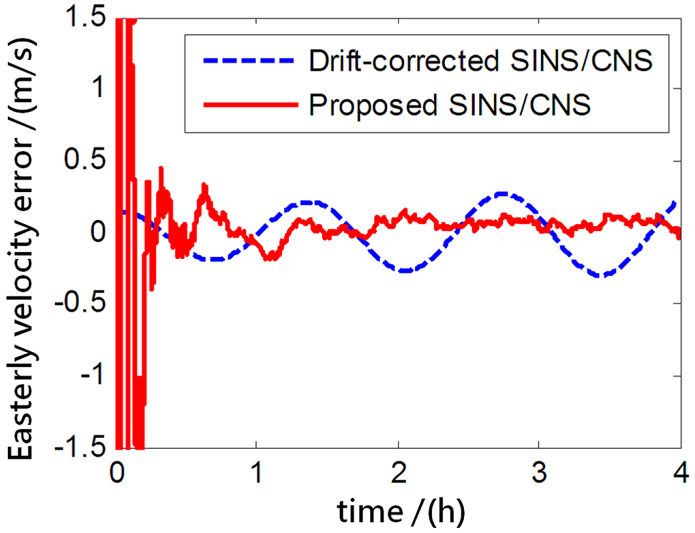
The performance of the proposed SINS/CNS integrated navigation system are compared with that of a traditional gyro-drift-corrected SINS/CNS integrated system, as shown in Figures 8–16. In order to distinguish different simulation results of the two integration schemes, red curves are used to express the results of the proposed navigation scheme and blue curves illustrate the results of the traditional gyro-drift-corrected SINS/CNS scheme. Figures 8 –10 illustrate the position errors of the proposed SINS/CNS scheme and the drift-corrected SINS/CNS scheme. Figures 11–13 compare the velocity error, and attitude error is shown in Figures 14–16. Table 5 shows the performance precision comparison between the gyro-drift-corrected SINS/CNS scheme and the proposed scheme (including variance and maximum value of navigation error).

Figure 8. Easterly position error.

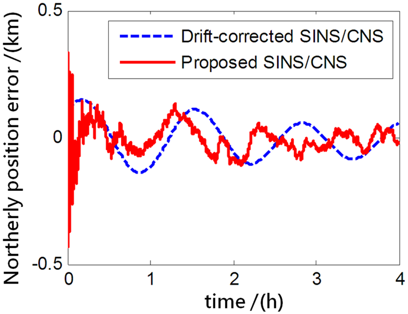
Figure 9. Northerly position error.

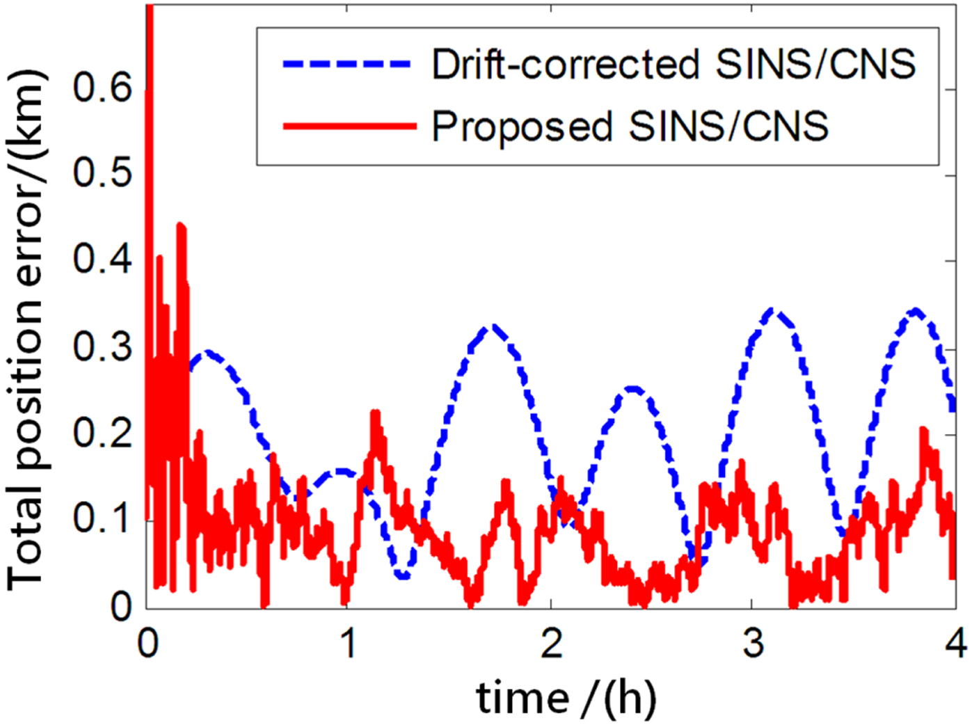
Figure 10. Total position error.

Figure 11. Easterly velocity error.

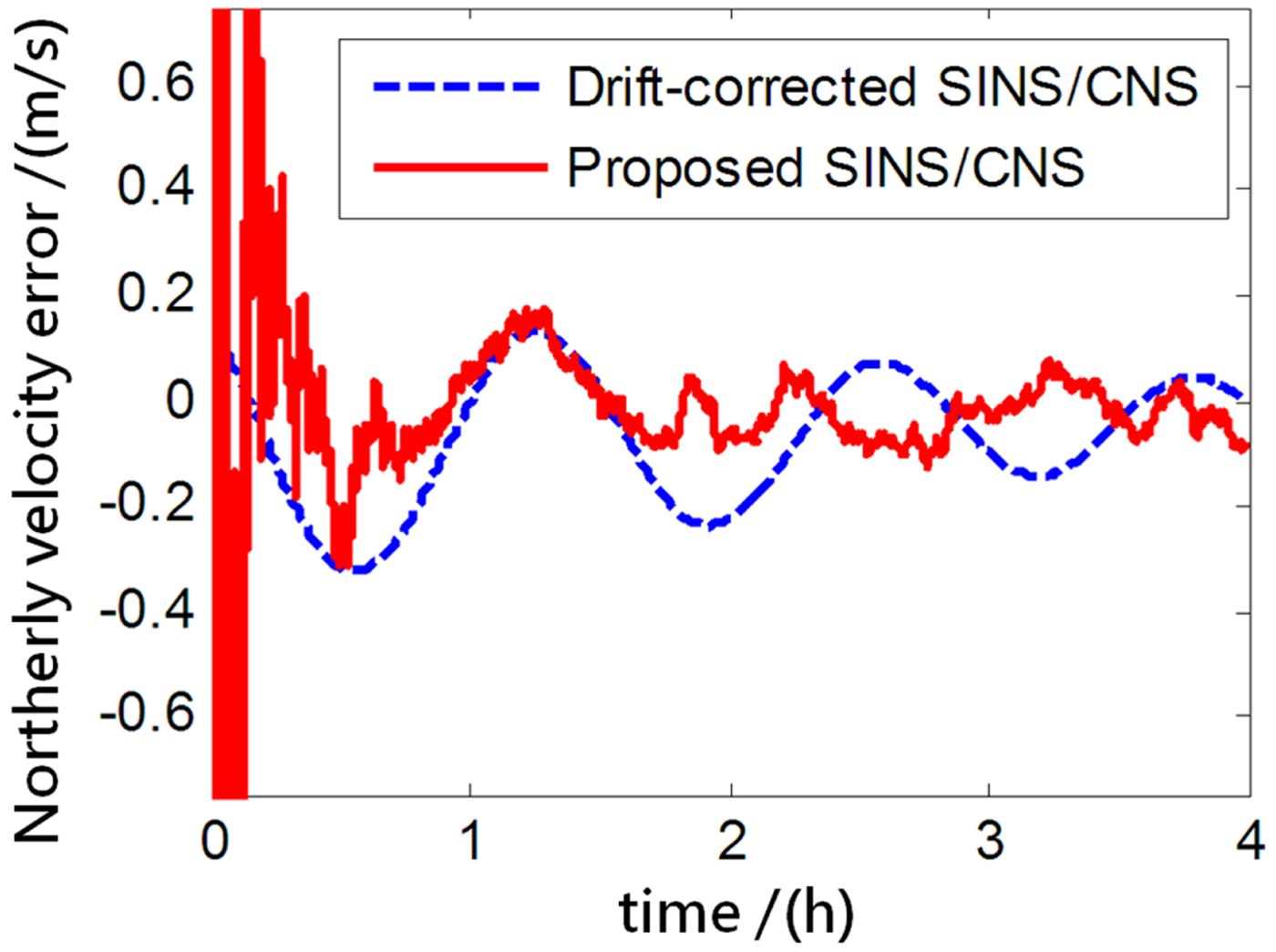
Figure 12. Northerly velocity error.

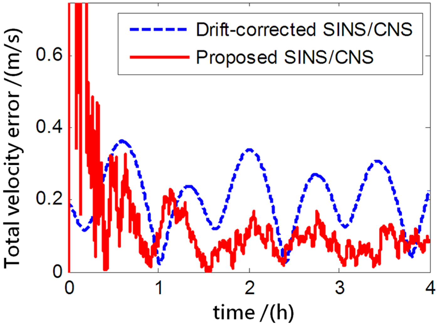
Figure 13. Total velocity error.

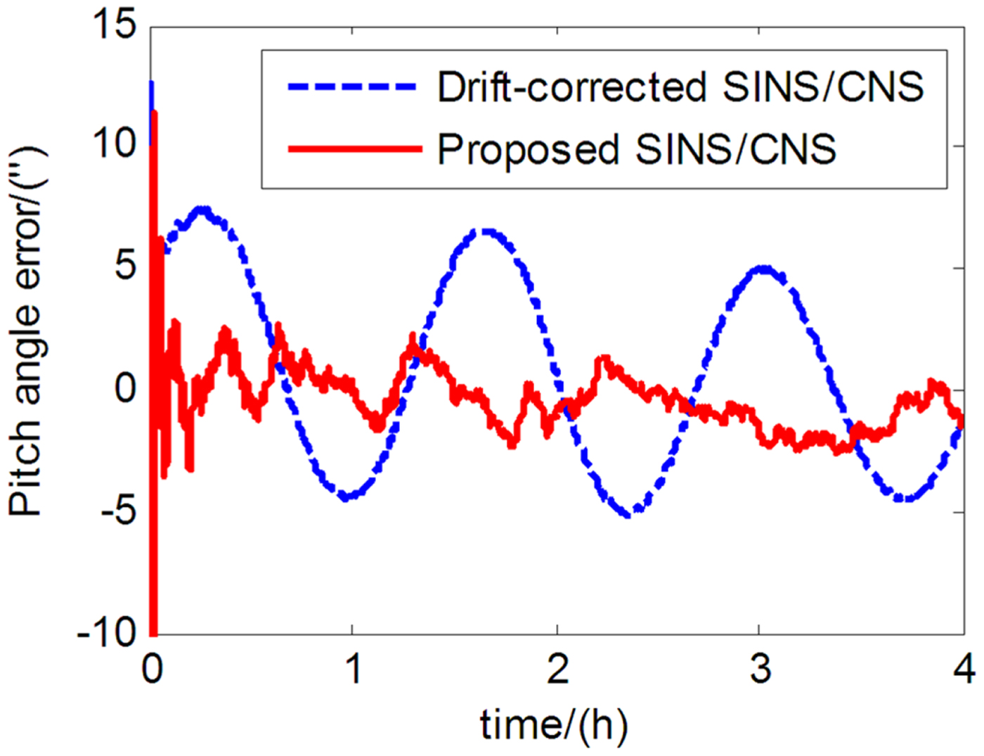
Figure 14. Pitch angle error.

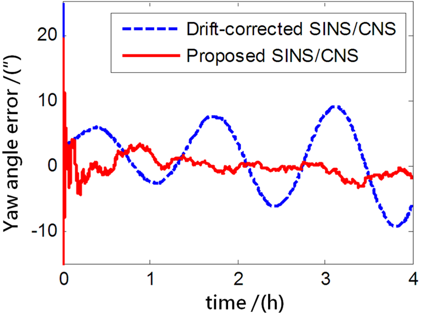
Figure 15. Yaw angle error.

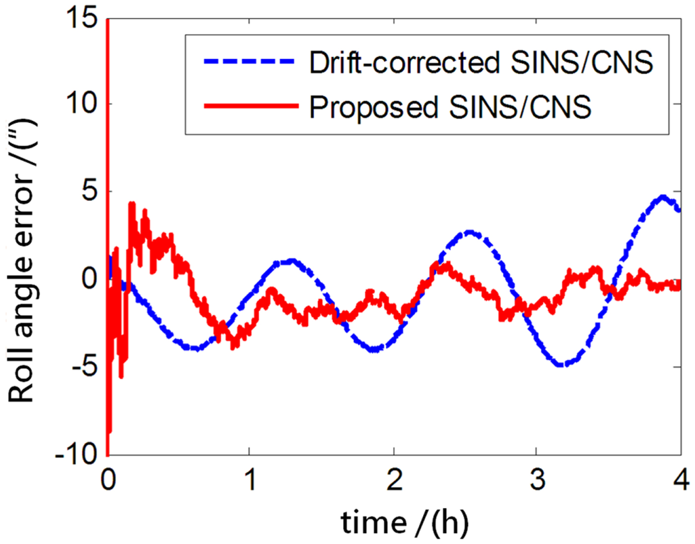
Figure 16. Roll angle error.

Table 5. Simulalion results of two different integration modes.

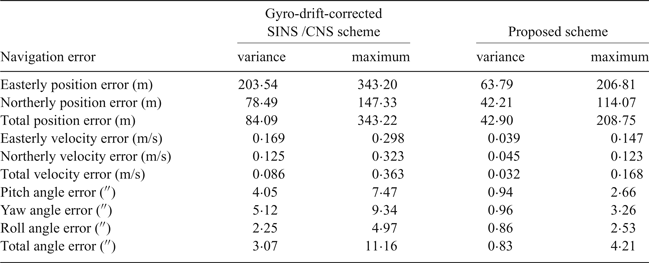
As the blue curves show in Figures 8–10, the position errors of the gyro-drift-corrected SINS/CNS scheme are gradually diverging with time and the maximum total position error reaching 343·20 m, as shown in Table 5. However, as shown in the red curves, it is clear that the position errors of the proposed SINS/CNS scheme are sharply reduced. With the aid of CNS, the maximum total position error is reduced to 208·75 m. Velocity accuracy of the proposed scheme is also improved as shown in the curves in Figures 11–13. Compared with the gyro-drift-corrected scheme, velocity error of the proposed scheme does not diverge, and the maximum error is reduced from 0·363 m/s to 0·168 m/s, as shown in Table 5. Figures 14–16 show a comparison of attitude errors in the two different schemes. As is shown in the blue curves, attitude errors of the gyro-drift-corrected scheme diverge due to an inaccurate horizontal reference. So, the attitude accuracy becomes poor and the maximum error is more than 10$^{\prime\prime}$. As the CNS can provide an accurate horizontal reference, attitude errors of the proposed SINS/CNS converge quickly and remain at about 5$^{\prime\prime}$, as shown in the red curves. Therefore, through the aiding given by the CNS, the accuracy of SINS/CNS is significantly improved.