


1. INTRODUCTION
In helicopter operations, accident investigation has been vital to the development of safety measures. Research has shown that different types of mission are exposed to specific risk factors, with the conclusion that mission-based analysis of accidents is essential for their prevention. A significant proportion of helicopter missions involve activities in the oil and gas industry. Within these, offshore operations comprising missions to, from and between installations at sea (Simons et al., Reference Simons, Wilschut and Valk2011), are critical. With over nine million passengers transported worldwide annually, it is a major concern that helicopters are the largest contributors to the overall risk of fatal accidents in the offshore oil and gas industry (OGP, 2012).
Despite the recognised need, there is no comprehensive mission-tailored accident analysis framework for the helicopter industry. This paper aims to develop such a framework and implement it to evaluate the characteristics of offshore helicopter accidents. The next section reviews previous helicopter accident research. Section 3 builds on the review to specify the architecture of the framework, which is implemented in Section 4. The results are presented and discussed in Section 5, before conclusions are drawn in Section 6.
2. STATUS OF HELICOPTER SAFETY ANALYSIS
Currently, there are three methods used for the analysis of helicopter accidents: (i) adapted from fixed-wing operations, (ii) based on non-mission related risk factors (e.g., per helicopter category), and (iii) mission-specific. The first has the weakness of introducing significant biases in the results, necessitating the application of complimentary taxonomies (EHEST, 2010). Although developed for helicopter accident analysis, the second method is only able to provide conclusions at a high level (Majumdar et al., Reference Majumdar, Mak, Lettington and Nalder2009). The existing mission-tailored frameworks focus on simple frequency counts and do not adequately explore the statistical interactions between risk factors (OGP, 2012).
A common drawback of these methods is the low quality of accident data used which limits statistical analysis (Nascimento et al., Reference Nascimento, Majumdar and Ochieng2012b). For example, excessively large analysis timeframes have compromised data timeliness and identified risk factors of low relevance to current operations (Harris, Reference Harris2006). Additionally, the inconsistent use of terminological definitions has led to the incomplete sampling of accidents (Williams, Reference Williams2012). In addition to incompleteness in general, the collection of the appropriate amount of data has been affected by sampling strategies constrained by political jurisdictions (EHEST, 2010).
Despite these limitations, the current methods have been useful in identifying a number of risks in offshore helicopter operations. These include night-time and arrival segments, both associated with a range of contextual factors that may negatively impact the pilots' ability to fly, particularly in developing countries (Nascimento et al., Reference Nascimento, Majumdar and Jarvis2012a, Reference Nascimento, Majumdar, Ochieng and Jarvis2012c). The use of single engine aircraft is also a well-established risk (Nascimento et al., Reference Nascimento, Majumdar and Ochieng2012b).
In order to understand fully the risks in the helicopter domain, a robust analysis framework is required. The next section proposes a new framework that accounts for the weaknesses identified above, and uses it for the analysis of accidents in offshore helicopter operations. The results are compared to the known risks to ensure validity.
3. FRAMEWORK DEVELOPMENT
Figure 1 captures the architecture of the new framework.

Figure 1. Analysis framework.
Initially, the selection of an appropriate timeframe for the analysis is required. This is followed by a precise definition of terms, the identification of relevant countries and the sources of accident and operational data. The next step involves the definition of the variables for accident analysis and the calculation of accident rates together with consideration of data completeness issues. Finally, a three-fold statistical analysis strategy is executed. This comprises the analysis of accident rates together with bivariate and multivariate analyses across the relevant variables. Each step is described in detail in the following sections.
3.1. Timeframe selection
In order to ensure relevance to current operations, the timeframe selected should be representative of both the technologies and operating conditions (e.g. helicopter types used). Selection might be attempted by consulting summaries of helicopter activity issued by institutions of international reach e.g. International Association of Oil and Gas Producers (OGP, 2012), national aviation authorities of countries that focus on the type of mission under study and helicopter accident studies (e.g. EHEST, 2010).
3.2. Definition of terms
This assures the comparability of data issued by different sources and should include definitions at a high level, where needed.
3.3. Identification of relevant countries
Given that international treaties require national authorities to be responsible for accident investigations, analysis of helicopter accidents requires the identification of the countries where the mission of interest is known or expected to occur. The sources mentioned in Section 3.1 can be used for country identification.
3.4. Operational data collection
Accident rates enable interpretation of accidents with regards to the size of operations. Therefore, the sources of such data should be identified (Section 3.1) and the variables to be used for the calculation of accident rates selected. For example, although flying hours typically estimate time at risk, other metrics reflect alternative safety perspectives, e.g. cycles of take-off and landing (Oil and Gas UK, 2011). Data completeness checks are required to assess the quality of such data (Nascimento et al., Reference Nascimento, Majumdar and Ochieng2012b) and to make recommendations for improved data collection and dissemination where needed.
3.5. Accident data collection
The reports issued by national accident investigation authorities might be complemented by those published by unofficial sources (e.g. those in Section 3.1). From such sources and the literature, variables of potential relevance to accidents (e.g. phases of flight) should be identified and a bespoke cause classification scheme developed. This might start from existing mature classification schemes (e.g. that of the European Coordination Centre for Accident and Incident Reporting Systems – ECCAIRS), which can be adapted as necessary to capture the finest possible level of detail with respect to the factors associated with the occurrences. However, given the potentially different accident models and investigation stop rules employed by the original accident investigators, varying levels of detail might be reported, which may prevent causal analysis at the desired level of detail. Following data extraction, completeness checks are applied.
3.6. Statistical analysis
In order to understand complex relationships and make inferences about unpredictable data (e.g. accidents), rigorous statistical analysis is required. A three-fold analysis plan is desirable as this enables the examination of accident characteristics from different and complimentary viewpoints. A bivariate analysis follows the analysis of rates to confirm the results obtained, investigate the variables for which accident rates are unavailable or inapplicable and cover any gaps caused by suboptimal quality data. Subsequently, a multivariate analysis identifies the multi-way interactions among variables and generates predictions based on past accident data. The tests to be applied depend on the characteristics and distributions of the data. Section 4 presents the tests used in this paper during the implementation of the framework.
4. FRAMEWORK IMPLEMENTATION
Stakeholders in the oil and gas industry are renowned for their efforts to improve safety in the sector. Therefore, the data used in this paper are potentially of the highest quality currently achievable in the helicopter domain. However, several shortcomings were identified as described below.
4.1. Timeframe selection
Worldwide offshore helicopter operations between 1997 and 2011 fulfilled the conditions outlined in Section 3.1 (Oil and Gas UK, 2011).
4.2. Definition of terms
The accident statistics of offshore helicopter operations are frequently understated since the USA National Transportation Safety Board (NTSB) does not classify certain catastrophic types of occurrences as “accidents” (Williams, Reference Williams2012). To overcome this, the International Civil Aviation Organisation's (ICAO) definition of accident is refined in this paper as follows:
“An accident is an occurrence associated with the operation of an aircraft which takes place between the time any person boards the aircraft with the intention of flight until such time as all such persons have disembarked, (a) in which a person is fatally or seriously injured as a result of: being in the aircraft; or direct contact with any part of the aircraft; or direct exposure to jet blast; or (b) as a consequence of which, at any time until recovery, the aircraft sustains damage or structural failure which: adversely affects the structural strength, performance or flight characteristics of the aircraft and would normally require major repair or replacement of the affected component; or (c) in which the aircraft is missing or is completely inaccessible.”
This definition addresses flights over other hostile environments (e.g. rough seas) that might destroy aircraft after relatively successful forced landings. The need to account for this aspect of helicopter operations has led to on-going revisions of regulations (e.g. EASA, 2012).
4.3. Identification of relevant countries
A total of 50 countries were identified from summaries of petroleum activity (BP, 2010) and helicopter safety analyses.
4.4. Operational data collection
Public domain data were complete to support the calculation of rates only for flight hours between 1997 and 2009 (OGP, 2012). The calculation of daylight and night-time flying hours was based on estimates whereby 3% of the worldwide and 8·46% of North Sea's total annual flying hours occur at night (Nascimento et al., Reference Nascimento, Majumdar and Ochieng2012b). The remainder of the night-time flying hours were split between the remaining flying regions (see Section 4.6.1) in proportion to the total flying hours in each region.
4.5. Accident data collection – sources and sampling strategy
Accident information was sought from the reports issued by the official accident investigation authorities of the 50 relevant countries. Of these, 46 target databases were available online. Checking the accident information gathered against the analyses outlined in Section 2 was needed, as typically, developing countries did not share accident information online.
Given the definition of an accident adopted, additional revision of the reported incidents in the countries of interest was needed. All the incidents available from the 46 databases were checked, as well as those reported to the USA's Accident/Incident Data System (AIDS) (FAA, 2012), Canadian Civil Aviation Daily Occurrence Reporting System (CADORS) (Transport Canada, 2012), British Mandatory Occurrence Reporting (MOR) scheme and Australian Transportation Safety Bureau (ATSB). The search words of Baker et al. (Reference Baker, Shanahan, Haaland, Brady and Li2011) were used, complemented by “ditching”, “water landing”, “oil”, “gas” and “ship”. This led to the incorporation of 16 catastrophic ditching “incidents” into this paper's “accident” dataset, all in the USA. The destruction of such helicopters was confirmed by checking the FAA aircraft registry.
Further searches were conducted using websites specialised in the sharing of aircraft-related information (e.g. Flight Safety Foundation, 2012). To minimise uncertainties, only accidents that matched the definition used in this paper and reported by at least two independent sources were included. Finally, the non-specialised press was checked for non-technical information e.g. if the accident occurred at night.
4.6. Identification of variables relevant to accidents and data completeness
A total of 139 variables of potential relevance to accidents were identified. Of these, 63 variables covered the demographic characteristics of each pilot (e.g. age) and 13 described the operating environment (e.g. meteorological conditions, cockpit instrumentation and autopilot fit). With the threshold for data completeness established at 90% (worldwide and across each regional dataset), the variables included in the analyses are outlined below.
4.6.1. Regions of occurrence
Instead of focussing on an artificial per-country grouping strategy, this paper uses the following OGP classification of offshore helicopter areas based upon the similarity of operational characteristics (OGP, 2012):
• Gulf of Mexico (GOM);
• North Sea (NS);
• Other regions.
Since “other regions” encompassed areas of dissimilar characteristics (e.g. typical weather conditions in Canada and Africa), re-clustering was required. This was based on aspects relevant to safety that were derived from Nascimento et al. (Reference Nascimento, Majumdar, Ochieng and Jarvis2012c), as shown in Table 1.
Table 1. Clustering of “other regions”.
1 Accidents happened in Saudi Arabia, United Arab Emirates, Iran and Qatar.
2 Accidents happened in China, Taiwan, Indonesia, Thailand, Malaysia and Myanmar.
3 Commonwealth of Independent States. Accidents happened in Azerbaijan, Russia and Ukraine.
4 Accidents happened in Angola, Nigeria, Congo and Cameroon.
5 See Table 2.
Table 2. Helicopter category classification scheme.
4.6.2. Aircraft categories
Given differences in engine reliability (Harris, Reference Harris2006), the OGP's classification scheme for helicopter categories (OGP, 2012) was slightly modified (i.e. single engine helicopters were split into piston or turbine powered) and used. As Table 2 shows, the scheme mostly concerns the number of passengers transported.
4.6.3. Phases of flight
The phases of flight used in this paper account for the physical loads imposed on offshore helicopters and the cognitive effort of pilots (Teixeira, Reference Teixeira2006). However, the lack of detail in a considerable part of the dataset led to the clustering of phases as in Table 3. Despite the reduced ability to discriminate phases of flight, such clustered phases closely matched those of the UK Civil Aviation Authority (CAA, 2005), indicating their external validity.
Table 3. Flight phases classification scheme.
4.6.4. Lighting conditions
Previous helicopter safety studies used time blocks to infer luminescence, e.g. with night-time assumed between 19:00 and 07:00. Because lighting cycles may vary considerably throughout the year, especially at high latitudes, the astronomical almanac was used to calculate the civil twilights at the locations and dates of the accidents (Nascimento et al., Reference Nascimento, Majumdar and Ochieng2012b). Subsequently, the accidents were classified as having occurred in daylight (i.e. between the morning and evening civil twilights) or at night.
4.6.5. Outcomes
These were used to establish event severity (i.e. fatal or not).
4.7. Development of accident cause classification scheme
Given the need to account for varying levels of detail reported by the different sources, the cause classification scheme reflected the finest level of detail found across the whole dataset, and hence took the high-level form presented in the Appendix. Causes were attributed to the “precipitating factor” or “the first event” that initiated the accident (Oil and Gas UK, 2011; Harris, Reference Harris2006, respectively). It is important to note that limited accident datasets do not allow for complex multivariate causal analysis (Majumdar et al., Reference Majumdar, Mak, Lettington and Nalder2009).
The findings of the original accident investigations were categorised using the scheme. For accidents without official investigation reports, the findings reported by the OGP were accepted on the basis of privileged information, e.g. from insurance claims. The remaining accidents were discussed among the authors and a conservative approach taken by frequently assigning “unknown or unavailable” as the accident cause. Most such accidents were the catastrophic ditchings originally classified as incidents, and hence not subject to complete investigations. The accidents stemming from operational causes were further classified as pilot-related whenever the reports indicated that they could have been avoided by appropriate piloting. However, this is not labelling such accidents as caused by pilot errors, as this labelling has previously been found premature and inconsistent across official accident reports (e.g. Hollnagel, Reference Hollnagel2009). This classification highlights opportunities for developing pilot-supportive tools (e.g. better automation modes).
4.8. Statistical analysis
For all the statistical tests, significance was established at p<0·050.
4.8.1. Analysis of accident rates
Given the sample sizes involved, the Shapiro-Wilk and Levene tests were used to check the normality of the distributions and the homogeneity of variance, respectively. Because in all cases at least one such assumption of parametric data was violated, non-parametric techniques were required. See Field (Reference Field2009) and Agresti (Reference Agresti2002) for details of the statistical tests mentioned above and outlined below.
4.8.1.1. The Kolmogorov-Smirnov Z (KS-Z) procedure
This procedure tested the null hypothesis whereby the distributions of accident rates across two conditions (i.e. daytime and night-time) were the same. Such a test ranks the data points in ascending order in each group separately and calculates the maximum absolute difference (D) between the observed cumulative distribution functions for both samples. The test is useful with small sample sizes, i.e., N<25 per group and its statistic is calculated as shown below, where n 1 and n 2 are the sample sizes in each condition.
 $$Z = {\rm max} _{\,j| D_j |} \sqrt {\displaystyle{{n_1 n_2} \over {n_1 + \; n_2}}} $$
4.8.1.2. The Moses Test of Extreme Reaction (MTER)
This investigated the null hypothesis that the extreme values observed for accident rates were equally likely to occur in both conditions studied (i.e., daytime and night-time). In this test, observations from both conditions are combined and ranked, and the probability, under the null hypothesis, that the range (r) of the control condition (i.e., daytime) is not greater than the observed range (m+k) is calculated by the following equation:
 $$P(r \le m + k) = \; \displaystyle{{\mathop \sum \nolimits_{i = 0}^k \left( {\matrix{ {i + m - 2} \cr i \cr}} \right)\left( {\matrix{ {n + 1 - i} \cr {n - i} \cr}} \right)} \over {\left( {\matrix{ {m + n} \cr m \cr}} \right)}}$$
where m and n are the number of observations in the control and experimental groups respectively (Sprent and Smeeton, Reference Sprent and Smeeton2001).
4.8.1.3. Kruskal-Wallis (KW)
This procedure tested the null hypothesis that the distributions of accident rates across k experimental conditions (i.e. the regions of occurrence) were the same. In this test, observations for all groups are jointly sorted and ranked and, for each group, the sum of ranks R i and the number of observations n i is obtained. With N as the total sample size, the test statistic is computed as:
 $$H = \; \displaystyle{{12} \over {N(N - 1)}}\; \mathop \sum \limits_{i = 1}^k \displaystyle{{R_i^2} \over {n_i}} - 3\; (N + 1)$$
where H follows a chi-square distribution with (k−1) degrees of freedom. In case significant results are found, post-hoc tests are used to identify where the differences lie, as described below.
4.8.1.4. The Mann-Whitney test with Bonferroni correction (MW/B)
This test was applied to each pair-wise combination of conditions drawn from the previous step to test the null hypothesis whereby the two samples were from populations with the same distribution functions. In this test, the observations in both groups are combined and ranked. The number of times that a score from one group precedes a score from the other group, and vice versa, is then calculated. The Mann-Whitney U statistic is the smaller of these two numbers, given by the following equation:
 $$U = \; n_1 n_2 + \; \displaystyle{{n_1 (n_1 + 1)} \over 2} - \; R_1 $$
where n 1 and n 2 are the sample sizes of both groups being compared, R 1 is the sum of ranks for group 1 (assumed with the smallest U), and the significance levels of U are given by specific algorithms. The Bonferroni correction avoids falsely rejecting the null hypothesis by using a more stringent rejection criterion given by the initial significance level divided by the number of pairs under analysis. Because it consistently presented the lowest and most spaced-in-time accident rates, the North Sea was chosen as the control group for these tests.
4.8.2. Bivariate accident analyses
The Pearson's chi-square test was applied to investigate the null hypothesis whereby the categorical variables were independent when analysed in pairs. Based on the binomial distributions of marginal frequencies, this test compares the actual counts across the events of the variables with the counts that would be expected if the variables were independent. The greater the discrepancy, the larger the dependency (also called “association”). The discrepancy is calculated by the chi-square statistic, as follows:
 $${\rm X}^2 = \mathop \sum \limits_{i = 1}^r \mathop \sum \limits_{\,j = 1}^k \displaystyle{{(n_{{\rm ij}} - \mu _{{\rm ij}} )^2} \over {\mu _{{\rm ij}}}} $$
where n ij and μ ij are the observed and expected frequencies, and i and j represent rows and columns in the contingency tables, respectively. This test requires that not less than 80% of the cells in such tables have expected frequencies greater than five and that no single expected frequency is lower than unity. When this was violated, Fisher's exact test was used. This calculates exact probabilities based on the hyper-geometric distribution of inner cell counts. In both cases, clustering of categories was needed to avoid null cell frequencies. For example, the Single Engine (SE) category was formed from the fusion of SP and ST, and LT/MT was formed from the fusion between LT and MT. Furthermore, the “ground manoeuvres” category was created from the fusion between the parked and taxiing flight phases, and the “arrival segment” was formed from the fusion between approach and landing.
4.8.3. Multivariate accident analysis
Given the characteristics of the data, the exploration of possible interactions between more than two accident variables was embedded in the logistic regression analysis. This was used to predict the events of dependent variables (i.e., causes and outcomes of accidents) by modelling the linear relationship between the natural logarithm of the odds of such variables and the explanatory variables i.e., regions of operation, aircraft categories, phases of flight, lighting conditions and all possible interactions between such variables in the former case; and such variables, accident causes and all possible interactions between these variables in the latter case. The odds are defined as the ratio between the probability of an event of the dependent variable occurring (i.e., π) over the probability of such event not occurring (i.e., 1-π). The logistic regression is expressed as follows:
 $$\ln (\pi /1 - \pi ) = b_0 + \mathop \sum \limits_{i = 1}^{\rm n} b_i X_i $$
where b o is the constant and X i are the explanatory variables with their coefficients b i. Such a regression, frequently used in transport research, uses maximum likelihood estimation to maximise the probability of obtaining the observed results given the fitted regression coefficients.
In order to ensure that the standard errors of the b coefficients were not excessively large, unobserved combinations of predictors needed to be avoided. This required further clustering of categories (e.g., LT, MT and HT clustered into the Multi-Engine (ME) category). The forward stepwise model fitting strategy based on the log-likelihood statistic was used to account for the exploratory nature of this study. Overdispersion and multicollinearity were not present in the data.
5. RESULTS
The sampling strategy returned 189 accidents, 65% of which were covered by official investigations. The OGP summaries accounted for a further 25%, leaving 10% to the judgement of the authors. The accidents with “unknown/unavailable” information were excluded from the analysis. Accident information was normalised by the flying hours data available (i.e. 1997–2009) and discriminated by four regions of operations, three lighting conditions, seven causes and two outcomes. The bivariate and multivariate analyses of accident data covered the whole (1997–2011) period. The analyses are presented and interpreted in the following sections.
5.1. Analysis of accident rates
Figure 2 illustrates the worldwide overall and fatal accident rates (blue solid and red dotted lines, respectively) for all causes, grouped according to lighting conditions (daytime to the left, night-time to the right). The much higher accident rates in the night-time are noticeable.

Figure 2. Worldwide overall and fatal accident rates (blue solid and red dotted lines, respectively) for all causes, per lighting conditions (daytime to the left, night-time to the right).
The results of the statistical tests applied are summarised in Table 4, which also outlines the hypotheses tested. The fact that worldwide night-time accident rates were either significantly greater (test of hypothesis H01, KS-Z tests) or tended towards the extreme of the distributions (test of H02, MTER) for all combinations of causes and outcomes confirmed the trends in Figure 2, with the GOM and other regions following a similar pattern. However, for the NS the distributions per lighting condition were not significantly different (KS-Z tests), indicating comparable risk levels in this region. Nonetheless, since all the ranges were significantly different (MTER), any helicopter accident at night inflated the accident rates, and should therefore be addressed.
Table 4. Results of the tests applied to accident rates.

KS-Z Kolgomorov-Smirnov Z test.
MTER Moses Test of Extreme Reaction.
KW Kruskal-Wallis test.
MW/B Mann-Whitney test with Bonferroni correction.
✓ Significant result: reject H0.
X Non-significant: accept H0.
NA Not applicable.
Regarding the analysis per region (i.e., the test of H03), Table 4 shows that the distributions of accident rates (overall and fatal) for all causes were significantly different for the “whole day” condition with diverging post hoc analysis results. Whereas GOM's overall accident rates were significantly greater, the highest fatal accident rates occurred in the “other regions”. Further analysis per lighting condition indicated that the accident rates of the GOM were related to daytime operations. Conversely, the “other regions” sustained the highest night-time accident rates. This emphasises the night-time as a recognised condition for fatal helicopter accidents (Simons et al., Reference Simons, Wilschut and Valk2011; Nascimento et al., Reference Nascimento, Majumdar, Ochieng and Jarvis2012c).
In relation to just the operational failures, the whole day and daytime accident rates of the GOM were significantly higher than in all other regions. Concerning the fatal accident rates, both GOM and “other regions” performed significantly worse than the NS for the whole day and in daylight. However, during the night-time the “other regions” had the highest fatal accident rates. This clarifies that the increased risk of night-time operations in “other regions” stemmed from fatal operational failures, especially pilot-related. In the case of technical failures, the daytime accident rates of the GOM were the highest caused by poor maintenance.
These considerably higher accident rates indicate the persistent problem of pilot performance in the night-time throughout the analysis timeframe. With significantly higher fatal accident rates, this problem was worst in regions other than the NS and GOM. In contrast, the GOM faced the highest accident and fatal accident rates in the daytime in relation to maintenance and pilot performance issues. A plausible explanation is that, by assigning “pilot/maintainer error” as a cause of accidents more frequently than investigative authorities of other regions do, the NTSB's premature accident investigation stop rules (Hollnagel, Reference Hollnagel2009) might have biased the results. Alternatively it might be that this region genuinely presented the harshest operating conditions to pilots/maintainers.
5.2. Bivariate accident analysis
The results are presented in Table 5. The association between regions of occurrence and aircraft category stemmed from significantly more accidents to HT aircraft in the Commonwealth of Independent States (CIS), than expected from independent variables. This was unsurprising since operations in this region are dominated by such helicopters. Regarding lighting conditions, night-time accidents occurred in higher frequencies in Africa, NS and Middle East, and in daylight in the GOM. Despite confirming that developing countries were less prepared to undertake night-time operations (Nascimento et al., Reference Nascimento, Majumdar and Jarvis2012a), the association with the NS suggests that more exposure to the night-time might be related to the occurrence of accidents. Again this highlights careful consideration of the use of helicopters over the sea at night.
Table 5. Results of the statistical tests applied to pairs of categorical variables.
✓ Significant association.
X Non-significant association.
Fatal accidents were more frequent in Africa, Americas except GOM, Australasia and CIS, and less frequent in the GOM. This confirms the results in Section 5.1 and explains why regulations and safety practices are more lenient in the GOM, with SE helicopters flying offshore and catastrophic ditchings still being classified as incidents.
The significant association between aircraft category and lighting condition occurred as MT helicopters crashed at night more often than expected. MT aircraft were also significantly associated with fatal accident outcomes, controlled flights into terrain or water (CFITWs) and tail rotor failures. Additionally, engine failure accidents were significantly associated with SP/ST aircraft. These associations indicate that MT helicopters were used in conditions that were excessively challenging to pilots, necessitating an examination of the helicopter's operational envelope. This is particularly important, as MT aircraft are the preferred choice for night-time missions, eg. medical evacuation, in many parts of the world.
Lighting conditions were associated with accident severity – with more fatal accidents at night – and causes, showing that night-time operational, pilot-related and CFITW accidents did not occur at random. Furthermore, there were fewer airworthiness failures at night than expected, which was unsurprising given that such failures tend to occur according to time exposure.
The association between flight phases and accident causes stemmed from a concentration of operational failures on the ground and arrival manoeuvres and pilot-related accidents, CFITW and obstacle strikes during the arrival. Also contributing to this association was the concentration of technical failures, especially airworthiness and tail rotor failures in the cruise phase. These results confirm the need to normalise technical failures by the flight hour and operational failures by the flight segment. Additionally, the results confirm the urgent need to address pilot performance shortcomings during arrival manoeuvres of offshore operations (Nascimento et al., Reference Nascimento, Majumdar, Ochieng and Jarvis2012c).
Finally, accident severity was associated with causes of accidents, confirming that CFITWs were mostly fatal.
5.3. Multivariate accident analyses
5.3.1. Multinomial logistic regression
Despite further clustering, it was not possible to predict accident causes at the most detailed level of the cause classification scheme due to an excessively large number of unobserved combinations of predictors (50%). Using the intermediate level of the scheme, a test of the full model against a constant only model indicated that the predictors reliably distinguished between accidents causes (χ2(14)=34·692, p=0·002). Overall prediction success was 61·1% (pilot-related: 82·0%; airworthiness: 53·2%; else: 3·8%).
Multi-way interactions between the variables were not found. When comparing the odds of having technical, airworthiness failures to those of operational, pilot-related failures, the Wald criterion showed that aircraft category, phase of flight and the interaction between lighting condition and aircraft category made significant contributions to prediction. The use of multi-engine aircraft produced an odds ratio that represented a 2·4% likelihood of airworthiness-related accidents over that of single-engine aircraft. Regarding phases of flight, the odds ratios of airworthiness failures during the arrival and departure segments indicated likelihoods of 37·8% and 20·9% respectively, in comparison to accidents in the remaining phases of flight (largely dominated by the cruise). Considering the interaction between aircraft category and lighting condition, the change in the odds indicated that multi-engine aircraft operated in daylight were 4803·8% times more likely to be involved in airworthiness failures than single-engine aircraft operated at night. However, given the large 95% confidence interval obtained, this should be interpreted with care.
The predictions of failures other than airworthiness-related were only successful in 3·8% of the cases and thus need to be interpreted with care. Table 6 summarises the results.
Table 6. Results of multinomial logistic regression.
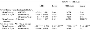
R2Mc Fadden=0·193; R2Cox & Snell=0·193; R2Nagelkerke=0·224 *p<0·050 **p<0·001
The results of the multinomial logistic regression were in general agreement with those of the bivariate analysis, barring the dissociation between lighting conditions and accident causes in the model. This could be an outcome of the clustering procedure that combined heterogeneous categories, thereby affecting prediction accuracy. Nevertheless, given the prediction successes achieved, the model is a good predictor of pilot-related events.
5.3.2. Binomial logistic regression
When predicting accident outcomes using the most-detailed level of the cause classification scheme, a test of the full model against a constant-only model indicated that the predictors as a set reliably distinguished between fatal and non-fatal accidents (χ2(3)=20·363, p=0·000). Overall prediction success was 72·9% (non-fatal: 94·9%; fatal: 24·5%).
Again, multi-way interactions between the variables were not found. The Wald criterion indicates that only lighting conditions and regions of operation made significant contributions to prediction (p=0·021 and p=0·006, respectively). When operating out of the GOM area, the odds ratio indicated that the likelihood of fatal accidents was 277% of that of the GOM. Similarly, when operating out of the NS area, fatal accidents were 256% as likely to happen. However, the confidence interval of the latter's odds ratio indicates the possibility of fewer fatal accidents occurring when moving out of the NS, e.g. in the GOM where there were proportionately fewer fatal accidents. A change in lighting condition from daytime to night-time produced an odds ratio corresponding to a fatal accident likelihood of 486%. Table 7 summarises the results.
Table 7. Results of binomial logistic regression.
R2Hosmer & Lemeshow=0·713; R2Cox & Snell=0·113; R2Nagelkerke=0·159 * p<0·05 ** p<0·01
The model predicted non-fatal outcomes more accurately than fatal outcomes and this may highlight a limitation in the use of regression analysis for accident data. The small sample size of fatal accidents may not support such analysis. This asks for novel ways of predicting accidents (Nascimento et al., Reference Nascimento, Majumdar, Ochieng and Jarvis2012c). Nevertheless, the model fitted and confirms the results of the previous analysis steps.
6. CONCLUSIONS
Given the mission-specific features of helicopter operations, there is a surprising lack of an analytical framework to systematically assess their risks with a view to mitigation. This paper has, for the first time, developed this framework and implemented it in the context of offshore operations in the oil and gas sector. This has resulted in the identification of a number of critical areas for priority intervention including the need for (i) improvement in the quality and sharing of accident data, (ii) new metrics for the normalisation of accidents, (iii) careful analysis of pilot performance at night and in the arrival flight segment, with a view to developing tools to support pilot tasks, and (iv) a new safety paradigm that accounts for the rarity of catastrophic accidents. The framework is designed to be transferable to other mission types, e.g. fire fighting, and thus is recommended for use across the gamut of existing missions.
ACKNOWLEGEMENTS
The ATSB and UK Civil Aviation Authority for data, and the Lloyd's Register Foundation for funding the research.
APPENDIX – ACCIDENT CAUSE CLASSIFICATION SCHEME


