2 Overview

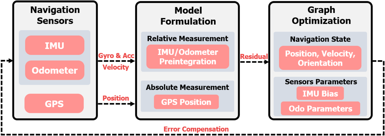
The structure of the proposed method is shown in Figure 1. The system is composed of navigation sensors, model formulation and graph optimisation. The navigation sensors consist of an IMU, odometer and GPS. The IMU provides gyros and accelerometers measurements while the odometer gives velocity measurements, which are used to form the IMU/odometer preintegration. Preintegration is a relative measurement that connects two successive states. The GPS position serves as an absolute measurement. The relative and absolute measurements are then used for building a residual error model. Finally, the navigation states and sensors parameters are estimated by the graph optimisation. The estimated parameters are sent to the navigation sensors to compensate for errors.

Figure 1. The structure of the proposed method

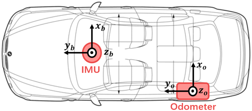
The IMU and odometer are mounted on different parts of a land vehicle, as shown in Figure 2. The odometer is installed on the rear wheel whose heading does not change during a manoeuvre. Above all, some coordinate systems need to be built to describe the spatial relationships among different measurements.

Figure 2. IMU and odometer frame

(1) IMU frame

The gyros and accelerometers are measured in the IMU frame, denoted as the $b$ frame. The three axes of the IMU frame are expressed as ${x_b}$, ${y_b}$ and ${z_b}$, which point to rightward, forward and upward, respectively. The IMU is mounted at one point of the land vehicle, so it misaligns with the vehicle body in practical situations. The IMU frame at instant $t$ is denoted as the ${b_t}$ frame.

(2) Odometer frame

The odometer frame is fixed on the land vehicle, denoted as the $o$ frame. The three axes of the odometer frame are represented by ${x_o}$, ${y_o}$ and ${z_o}$. The velocity measured by the odometer is in the moving direction of the vehicle, along the ${y_o}$ direction. The odometer frame at instant $t$ is denoted as the ${o_t}$ frame.

(3) World frame

The world frame is denoted as the $w$ frame. The origin is located at the IMU at the initial instant and the three axes of the world frame point east, north and up, respectively. Meanwhile, some typical symbols that are used throughout the paper are defined in Table 1.

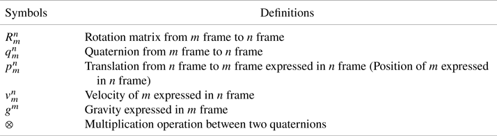
Table 1. Definitions of typical symbols

3 Derivation of IMU/odometer preintegration

In this paper, the IMU preintegration is extended by incorporating odometer measurements. Different from existing IMU/odometer preintegrations, the complete IMU/odometer preintegration model is derived in consideration of the scale factor of the odometer, and misalignments in attitude and position between the IMU and odometer. The models of raw gyroscopes and accelerometers are given by

(1)\begin{equation} \begin{aligned} {{\hat w}_{{b_t}}} & = {w_{{b_t}}} + {b_{{w_t}}} + {n_w}\\ {{\hat a}_{{b_t}}} & = {l_{{b_t}}} + {b_{{a_t}}} + R_w^{{b_t}}{g^{w}} + {n_a} \end{aligned} \end{equation}

where ${\hat w_{{b_t}}}$ and ${\hat a_{{b_t}}}$ are IMU readings at instant $t$; ${w_{{b_t}}}$ and ${l_{{b_t}}}$ denote the true value of the angular rate and motion acceleration at instant $t$; and ${b_{{w_t}}}$ and ${b_{{a_t}}}$ represent the gyro and accelerometer bias. The rotation matrix from world frame to the ${b_t}$ frame is denoted by $R_w^{{b_t}}$ and ${g^{w}}$ denotes the gravity expressed in world frame. The noise in the gyros ${n_w}$ and accelerometers ${n_a}$ is assumed as Gaussian, ${n_w} \sim {N}( {0,\sigma _{{w}}^{2}} )$, ${n_a} \sim {N}( {0,\sigma _{{a}}^{2}} )$. The gyro bias and accelerometer bias are modelled as random walk, whose derivatives are Gaussian, ${n_{{b_w}}} \sim {N}( {0,\sigma _{{b_w}}^{2}} )$, ${n_{{b_a}}} \sim {N}( {0,\sigma _{{b_a}}^{2}} )$ (Qin et al., Reference Qin, Li and Shen2018):

(2)\begin{equation} \begin{aligned} {{\dot b}_{{w_t}}} & = {n_{{b_w}}}\\ {{\dot b}_{{a_t}}} & = {n_{{b_a}}} \end{aligned} \end{equation}

The model of the odometer is given by

(3)\begin{equation} {s_{{o_t}}}{\hat v_{{o_t}}} = {v_{{o_t}}} + {n_s} \end{equation}

where ${\hat v_{{o_t}}}$ is the odometer readings at instant $t$ and ${v_{{o_t}}}$ denotes the true value of odometer at instant $t$. The raw odometer measurements are affected by the scale factor ${s_{{o_t}}}$ and noise ${n_s}$. The noise is assumed as Gaussian, ${n_s} \sim {N}( {0,\sigma _s^{2}} )$. The scale factor is modelled as random walk, whose derivative is Gaussian, $n_{{s_o}} \sim {N}(0,\sigma _{{s_o}}^{2})$:

(4)\begin{equation} \dot s_{{o_t}} = n_{{s_o}}\ \end{equation}

The position of the odometer expressed in the world frame $p_o^{w}$ is given by

(5)\begin{equation} p_o^{w} = p_b^{w} + R_b^{w}p_o^{b} \end{equation}

where $p_b^{w}$ denotes the position of the IMU expressed in the world frame, $R_b^{w}$ represents the rotation matrix from the IMU frame to world frame and $p_o^{b}$ is the position of the odometer expressed in the IMU frame, which is the misalignment in position.

Given two instants ${t_k}$ and ${t_{k + 1}}$, the position, velocity and orientation states in the world frame can be propagated by the IMU and odometer measurements, which can be formulated as

(6)\begin{equation} \begin{aligned} p_{{b_{k + 1}}}^{w} & = p_{{b_k}}^{w} + v_{{b_k}}^{w}\Delta {t_k} + \int {\int_{t \in [ {{t_k},{t_{k + 1}}} ]} {( {R_{{b_t}}^{w}( {{{\hat a}_{{b_t}}} - {b_{{a_t}}} - {n_a}}) - {g^{w}}} )\,d{t^{2}}} }\\ v_{{b_{k + 1}}}^{w} & = v_{{b_k}}^{w} + \int_{t \in [ {{t_k},{t_{k + 1}}}]} {( {R_{{b_t}}^{w}( {{{\hat a}_{{b_t}}} - {b_{{a_t}}} - {n_a}}) - {g^{w}}})} \,dt\\ q_{{b_{k + 1}}}^{w} & = q_{{b_k}}^{w} \otimes \int_{t \in [ {{t_k},{t_{k + 1}}}]} {\frac{1}{2}} \Omega ( {{{\hat w}_{{b_t}}} - {b_{{w_t}}} - {n_w}})q_{{b_t}}^{{b_k}}\,dt\\ p_{{b_{k + 1}}}^{w} & = p_{{b_k}}^{w} + R_{{b_k}}^{w}p_{{o_k}}^{{b_k}} + \int_{t \in [ {{t_k},{t_{k + 1}}} ]} {R_{{b_t}}^{w}R_{{o_t}}^{{b_t}}( {{s_{{o_t}}}{{\hat v}_{{o_t}}} - {n_s}} )\,dt} - R_{{b_{k + 1}}}^{w}p_{{o_{k + 1}}}^{{b_{k + 1}}} \end{aligned} \end{equation}

where

(7)\begin{equation} \Omega (w) = \left[\begin{array}{@{}cc@{}} - [w]_ \times & w\\ -w^{T} & 0 \end{array}\right],\quad [w]_ \times = \left[\begin{array}{ccc} 0 & { - {w_z}} & {{w_y}}\\ {{w_z}} & 0 & { - {w_x}}\\ { - {w_y}} & {{w_x}} & 0 \end{array} \right] \end{equation}

where $p_{{b_{k + 1}}}^{w}$ and $p_{{b_{k}}}^{w}$ denote the position of IMU expressed in the world frame at ${t_{k + 1}}$ and ${t_{k}}$, respectively; $v_{{b_{k + 1}}}^{w}$ and $v_{{b_{k}}}^{w}$ represent the velocity of the IMU expressed in the world frame at ${t_{k + 1}}$ and ${t_{k}}$, respectively; $q_{{b_{k + 1}}}^{w}$ and $q_{{b_{k}}}^{w}$ separately denote the quaternion from the ${b_{k + 1}}$ and ${b_{k}}$ frame to the world frame; $p_{{o_{k + 1}}}^{{b_{k + 1}}}$ and $p_{{o_k}}^{{b_k}}$ are misalignments in position at ${t_{k + 1}}$ and ${t_{k}}$; $R_{{b_{k + 1}}}^{w}$ and $R_{{b_{k}}}^{w}$ represent the rotation matrices from the ${b_{k + 1}}$ and ${b_{k}}$ frame to the world frame; $\Delta {t_k}$ is the duration between the time interval $[ {{t_k},{t_{k + 1}}} ]$; $R_{{b_t}}^{w}$ expresses the rotation matrix from the ${b_t}$ frame to the world frame; $R_{{o_t}}^{{b_t}}$ denotes the rotation matrix from the ${o_t}$ frame to the ${b_t}$ frame, which is the misalignment in attitude; and $q_{{b_t}}^{{b_k}}$ represents the quaternion from the ${b_t}$ frame to the ${b_k}$ frame.

The last equation in Equation (6) can be obtained from Equation 5) and the propagation of the position of the odometer expressed in the world frame, which can be formulated as

(8)\begin{equation} p_{{o_{k + 1}}}^{w} = p_{{o_k}}^{w} + \int_{t \in [ {{t_k},{t_{k + 1}}} ]} {R_{{b_t}}^{w}R_{{o_t}}^{{b_t}}( {{s_{{o_t}}}{{\hat v}_{{o_t}}} - {n_s}})\,dt} \end{equation}

where $p_{{o_{k + 1}}}^{w}$ and $p_{{o_{k}}}^{w}$ are the positions of the odometer expressed in the world frame at instants ${t_{k + 1}}$ and ${t_{k}}$, respectively.

It can be seen from Equation (6) that the propagation of the position from the odometer measurements requires the rotation and position at instant ${t_k}$. In the graph-optimisation-based algorithm, states at optimisation instants are frequently adjusted, which results in the odometer measurements needing to be re-propagated. To solve this problem, the preintegration theory is introduced into the odometer measurements.

The reference frame is changed from the world frame to the body frame at instant ${t_k}$. Equation (6) can be rewritten as

(9)\begin{equation} \begin{aligned} R_w^{{b_k}}p_{{b_{k + 1}}}^{w} & = R_w^{{b_k}}( {p_{{b_k}}^{w} + v_{{b_k}}^{w}\Delta {t_k} - \tfrac{1}{2}{g^{w}}\Delta t_k^{2}} ) + \alpha_{{b_{k + 1}}}^{{b_k}}\\ R_w^{{b_k}}v_{{b_{k + 1}}}^{w} & = R_w^{{b_k}}( {v_{{b_k}}^{w} - {g^{w}}\Delta {t_k}}) + \beta_{{b_{k + 1}}}^{{b_k}}\\ q_w^{{b_k}} \otimes q_{{b_{k + 1}}}^{w} & = \gamma_{{b_{k + 1}}}^{{b_k}}\\ R_w^{{b_k}}p_{{b_{k + 1}}}^{w} & = R_w^{{b_k}}p_{{b_k}}^{w} - R_w^{{b_k}}R_{{b_{k + 1}}}^{w}p_{{o_{k + 1}}}^{{b_{k + 1}}} + p_{{o_k}}^{{b_k}} + \eta_{{b_{k + 1}}}^{{b_k}} \end{aligned} \end{equation}

where

(10)\begin{equation} \begin{aligned} \alpha_{{b_{k + 1}}}^{{b_k}} & = \int {\int_{t \in [ {{t_k},{t_{k + 1}}} ]} {( {R_{{b_t}}^{{b_k}}( {{{\hat a}_{{b_t}}} - {b_{{a_t}}} - {n_a}} )} )} } \,d{t^{2}}\\ \beta_{{b_{k + 1}}}^{{b_k}} & = \int_{t \in [ {{t_k},{t_{k + 1}}} ]} {( {R_{{b_t}}^{{b_k}}( {{{\hat a}_{{b_t}}} - {b_{{a_t}}} - {n_a}} )} )} \,dt\\ \gamma_{{b_{k + 1}}}^{{b_k}} & = \int_{t \in [ {{t_k},{t_{k + 1}}} ]} {\frac{1}{2}} \Omega ( {{{\hat w}_{{b_t}}} - {b_{{w_t}}} - {n_w}} )\gamma_{{b_t}}^{{b_k}}\,dt\\ \eta_{{b_{k + 1}}}^{{b_k}} & = \int_{t \in [ {{t_k},{t_{k + 1}}} ]} {R_{{b_t}}^{{b_k}}R_{{o_t}}^{{b_t}}( {{s_{{o_t}}}{{\hat v}_{{o_t}}} - {n_s}} )\,dt} \end{aligned} \end{equation}

where $\alpha _{{b_{k + 1}}}^{{b_k}}$, $\beta _{{b_{k + 1}}}^{{b_k}}$ and $\gamma _{{b_{k + 1}}}^{{b_k}}$ denote the position, velocity and attitude preintegrations from the IMU measurements at instant ${t_{k + 1}}$ expressed in the ${b_k}$ frame; and $\eta _{{b_{k + 1}}}^{{b_k}}$ represents the position preintegration from the odometer measurements at instant ${t_{k + 1}}$ expressed in the ${b_k}$ frame. In Equation (10), the reference frame is ${b_k}$. Even though the states at instant ${t_k}$ are adjusted during the optimisation, the integrations in Equation (10) are not affected.

The discrete form of Equation (10) can be expressed as

(11)\begin{equation} \begin{aligned} \hat \alpha_{{b_{t + 1}}}^{{b_k}} & = \hat \alpha_{{b_t}}^{{b_k}} + \hat \beta_{{b_t}}^{{b_k}}\delta t + \tfrac{1}{2}\hat R_{{b_t}}^{{b_k}}( {{{\hat a}_{{b_t}}} - {{\hat b}_{{a_t}}}} )\delta {t^{2}}\\ \hat \beta_{{b_{t + 1}}}^{{b_k}} & = \hat \beta_{{b_t}}^{{b_k}} + \hat R_{{b_t}}^{{b_k}}( {{{\hat a}_{{b_t}}} - {{\hat b}_{{a_t}}}} )\delta t\\ \hat \gamma_{{b_{t + 1}}}^{{b_k}} & = \hat \gamma_{{b_t}}^{{b_k}} \otimes \left[\begin{array}{c} 1\\ \dfrac{1}{2}( {{{\hat w}_{{b_t}}} - {{\hat b}_{{w_t}}}} )\delta t \end{array} \right]\\ \hat \eta_{{b_t}}^{{b_k}} & = \hat \eta_{{b_t}}^{{b_k}} + \hat R_{{b_t}}^{{b_k}}\hat R_{{o_t}}^{{b_t}}{{\hat s}_{{o_t}}}{{\hat v}_{{o_t}}}\delta t \end{aligned} \end{equation}

where $\hat \alpha _{{b_{t + 1}}}^{{b_k}}$, $\hat \beta _{{b_{t + 1}}}^{{b_k}}$ and $\hat \gamma _{{b_{t + 1}}}^{{b_k}}$ are the preintegration from the IMU measurements at instant ${t_{t + 1}}$ expressed in the ${b_k}$ frame; $\hat \eta _{{b_{t + 1}}}^{{b_k}}$ denotes the preintegration from the odometer measurements at instant ${t_{t + 1}}$ expressed in the ${b_k}$ frame; $\hat \alpha _{{b_{t}}}^{{b_k}}$, $\hat \beta _{{b_{t}}}^{{b_k}}$ and $\hat \gamma _{{b_{t}}}^{{b_k}}$ are the preintegration from the IMU measurements at instant ${t_{t}}$ expressed in the ${b_k}$ frame; $\hat \eta _{{b_{t}}}^{{b_k}}$ denotes the preintegration from the odometer measurements at instant ${t_{t}}$ expressed in the ${b_k}$ frame; ${t_t},{t_{t + 1}} \in [ {{t_k},{t_{k + 1}}} ]$; $\delta t$ is the sampling interval of the IMU measurements; $\hat R_{{b_t}}^{{b_k}}$ represents the estimated rotation matrix from the ${b_t}$ frame to the ${b_k}$ frame; $\hat R_{{o_t}}^{{b_t}}$ denotes the estimated rotation matrix from the ${o_t}$ frame to the ${b_t}$ frame; and ${\hat b_{{a_t}}}$, ${\hat b_{{w_t}}}$ and ${\hat s_{{o_t}}}$ separately express the estimated accelerometers bias, gyros bias and scale factor of the odometer.

Then the continuous-time linearised dynamics of error term of Equation (10) can be written as

(12)\begin{align} \left[\begin{array}{@{}c@{}} {\delta \dot \alpha_{{b_t}}^{{b_k}}}\\ {\delta \dot \beta_{{b_t}}^{{b_k}}}\\ {\delta \dot \theta_{{b_t}}^{{b_k}}}\\ {\delta {{\dot b}_{{a_t}}}}\\ {\delta {{\dot b}_{{w_t}}}}\\ {\delta \dot \eta_{{b_t}}^{{b_k}}}\\ {\delta {{\dot s}_{{o_t}}}}\\ {\delta \dot p_{{o_t}}^{{b_t}}}\\ {\delta \dot \theta_{{o_t}}^{{b_t}}} \end{array} \right] & = \left[\begin{array}{ccccccccc} 0 & I & 0 & 0 & 0 & 0 & 0 & 0 & 0\\ 0 & 0 & { - \hat R_{{b_t}}^{{b_k}}{{[ {{{\hat a}_{{b_t}}} - {{\hat b}_{{a_t}}}}]}_ \times }} & { -\hat R_{{b_t}}^{{b_k}}} & 0 & 0 & 0 & 0 & 0\\ 0 & 0 & { - {{[ {{{\hat w}_{{b_t}}} - {{\hat b}_{{w_t}}}} ]}_ \times }} & 0 & { - I} & 0 & 0 & 0 & 0\\ 0 & 0 & 0 & 0 & 0 & 0 & 0 & 0 & 0\\ 0 & 0 & 0 & 0 & 0 & 0 & 0 & 0 & 0\\ 0 & 0 & { - \hat R_{{b_t}}^{{b_k}}{{[ {\hat R_{{o_t}}^{{b_t}}{{\hat s}_{{o_t}}}{{\hat v}_{{o_t}}}} ]}_ \times }} & 0 & 0 & 0 & {\hat R_{{b_t}}^{{b_k}}\hat R_{{o_t}}^{{b_t}}{{\hat v}_{{o_t}}}} & 0 & { - \hat R_{{b_t}}^{{b_k}}\hat R_{{o_t}}^{{b_t}}{{[ {{{\hat s}_{{o_t}}}{{\hat v}_{{o_t}}}} ]}_ \times }}\\ 0 & 0 & 0 & 0 & 0 & 0 & 0 & 0 & 0\\ 0 & 0 & 0 & 0 & 0 & 0 & 0 & 0 & 0\\ 0 & 0 & 0 & 0 & 0 & 0 & 0 & 0 & 0 \end{array} \right]\left[\begin{array}{c} {\delta \alpha_{{b_t}}^{{b_k}}}\\ {\delta \beta_{{b_t}}^{{b_k}}}\\ {\delta \theta_{{b_t}}^{{b_k}}}\\ {\delta {b_{{a_t}}}}\\ {\delta {b_{{w_t}}}}\\ {\delta \eta_{{b_t}}^{{b_k}}}\\ {\delta {s_{{o_t}}}}\\ {\delta p_{{o_t}}^{{b_t}}}\\ {\delta \theta_{{o_t}}^{{b_t}}} \end{array} \right]\nonumber\\ & \quad + \left[\begin{array}{cccccccc} 0 & 0 & 0 & 0 & 0 & 0 & 0 & 0\\ { - \hat R_{{b_t}}^{{b_k}}} & 0 & 0 & 0 & 0 & 0 & 0 & 0\\ 0 & { - I} & 0 & 0 & 0 & 0 & 0 & 0\\ 0 & 0 & I & 0 & 0 & 0 & 0 & 0\\ 0 & 0 & 0 & I & 0 & 0 & 0 & 0\\ 0 & 0 & 0 & 0 & { - \hat R_{{b_t}}^{{b_k}}\hat R_{{o_t}}^{{b_t}}} & 0 & 0 & 0\\ 0 & 0 & 0 & 0 & 0 & 1 & 0 & 0\\ 0 & 0 & 0 & 0 & 0 & 0 & I & 0\\ 0 & 0 & 0 & 0 & 0 & 0 & 0 & I \end{array} \right]\left[ \begin{array}{c} {{n_a}}\\ {{n_w}}\\ {{n_{{b_a}}}}\\ {{n_{{b_w}}}}\\ {{n_s}}\\ {{n_{{s_o}}}}\\ {{n_{{p_o}}}}\\ {{n_{{\theta_o}}}} \end{array} \right]\nonumber\\ & = {F_t}\delta z_{{b_t}}^{{b_k}} + {G_t}{n_t} \end{align}

where ${F_t}$ and ${G_t}$ represent the state transition matrix and noise matrix; $\delta z_{{b_t}}^{{b_k}}$ denotes the preintegration error vector in which the preintegration errors and sensor parameter errors are included; and $\delta \theta _m^{n}$ is the rotation error, which can be obtained by the following:

(13)\begin{equation} R_m^{n} = \hat R_m^{n}( {I + {{[ {\delta \theta_m^{n}}]}_ \times }}) \end{equation}

In Equation (12), the error term of misalignments in position and attitude are modelled as random walk, whose derivatives are Gaussian, ${n_{{p_o}}} \sim {N}( {0,\sigma _{{p_o}}^{2}} )$, ${n_{{\theta _o}}} \sim {N}( {0,\sigma _{{\theta _o}}^{2}} )$. According to Equation (12), the discrete form of error term can be formulated as

(14)\begin{equation} \delta z_{{b_{i + 1}}}^{{b_k}} = {F_{{d_{i + 1}}}}\delta z_{{b_i}}^{{b_k}} + {G_{{d_{i + 1}}}}n \end{equation}

where ${F_{{d_{i + 1}}}}$ and ${G_{{d_{i + 1}}}}$ represent the discrete state transition matrix and noise matrix, respectively. With the assumption that ${t_k}$ and ${t_{k + 1}}$ are two instants, ${t_i},{t_{i + 1}}, \ldots \in [ {{t_k},{t_{k + 1}}} ]$. Then, the transfer equation from instant ${t_k}$ to instant ${t_{k + 1}}$ can be written as

(15)\begin{align} \delta z_{{b_{k + 1}}}^{{b_k}} & = {F_{{d_{k + 1}}}} \cdots {F_{{d_{i + 1}}}}{F_{{d_i}}}\delta z_{{b_k}}^{{b_k}} + \xi\nonumber\\ & = {J_{{b_{k + 1}}}}\delta z_{{b_k}}^{{b_k}} + \xi \end{align}

where $\xi$ represents the other items for simplicity. Thus, the recursive equation of the state transition matrix ${J_{{b_i}}}$ and covariance matrix ${P_{{d_i}}}$ can be expressed as

(16)\begin{equation} \begin{aligned} {J_{{b_{i + 1}}}} & = {F_{{d_{i + 1}}}}{J_{{b_i}}}\\ {P_{{b_{i + 1}}}} & = {F_{{d_{i + 1}}}}{P_{{b_i}}}F_{{d_{i + 1}}}^{T} + {G_{{d_{i + 1}}}}QG_{{d_{i + 1}}}^{T} \end{aligned} \end{equation}

where $Q$ denotes the covariance matrix of noise, which is given by

(17)\begin{equation} Q = \left[\begin{array}{cccccccc} {\sigma_a^{2}} & 0 & 0 & 0 & 0 & 0 & 0 & 0\\ 0 & {\sigma_w^{2}} & 0 & 0 & 0 & 0 & 0 & 0\\ 0 & 0 & {\sigma_{{b_a}}^{2}} & 0 & 0 & 0 & 0 & 0\\ 0 & 0 & 0 & {\sigma_{{b_w}}^{2}} & 0 & 0 & 0 & 0\\ 0 & 0 & 0 & 0 & {\sigma_s^{2}} & 0 & 0 & 0\\ 0 & 0 & 0 & 0 & 0 & {\sigma_{{s_o}}^{2}} & 0 & 0\\ 0 & 0 & 0 & 0 & 0 & 0 & {\sigma_{{p_o}}^{2}} & 0\\ 0 & 0 & 0 & 0 & 0 & 0 & 0 & {\sigma_{{\theta_o}}^{2}} \end{array} \right] \end{equation}

According to Equation (15), the following can be obtained:

(18)\begin{align} {J_{{b_{k + 1}}}} & = {F_{{d_{k + 1}}}} \cdots {F_{{d_{i + 1}}}}{F_{{d_i}}}\nonumber\\ & = {F_{{d_{k + 1}}}} \cdots {F_{{d_{i + 1}}}}{F_{{d_i}}}I\nonumber\\ & = {F_{{d_{k + 1}}}} \cdots {F_{{d_{i + 1}}}}{F_{{d_i}}}{J_{{b_k}}} \end{align}

In the preintegration method, the reference frame is the IMU frame at instant ${t_k}$, which is ${b_k}$. The error term of preintegration at instant ${t_k}$ is $\delta z_{{b_k}}^{{b_k}}$, which means the error relative to itself. Thus, the initial values of Equation (16) can be set as (Qin et al., Reference Qin, Li and Shen2018)

(19)\begin{equation} \begin{aligned} {J_{{b_k}}} & = I\\ {P_{{b_k}}} & = 0 \end{aligned} \end{equation}

Thus, the Jacobian matrix ${J_{{b_{k + 1}}}}$ and covariance matrix ${P_{{b_{k + 1}}}}$ at instant ${t_{k + 1}}$ can be calculated by combining Equations (16) and (19). The correction equation for preintegration measurements can be expressed as the following form:

(20)\begin{equation} \begin{aligned} \tilde \alpha_{{b_{k + 1}}}^{{b_k}} & = \hat \alpha_{{b_{k + 1}}}^{{b_k}} + J_{\delta {b_{{a_k}}}}^{\delta \alpha_{{b_{k + 1}}}^{{b_k}}}\delta {b_{{a_k}}} + J_{\delta {b_{{w_k}}}}^{\delta \alpha_{{b_{k + 1}}}^{{b_k}}}\delta {b_{{w_k}}}\\ \tilde \beta_{{b_{k + 1}}}^{{b_k}} & = \hat \beta_{{b_{k + 1}}}^{{b_k}} + J_{\delta {b_{{a_k}}}}^{\delta \beta_{{b_{k + 1}}}^{{b_k}}}\delta {b_{{a_k}}} + J_{\delta {b_{{w_k}}}}^{\delta \beta_{{b_{k + 1}}}^{{b_k}}}\delta {b_{{w_k}}}\\ \tilde \gamma_{{b_{k + 1}}}^{{b_k}} & = \hat \gamma_{{b_{k + 1}}}^{{b_k}} \otimes \left[ \begin{array}{c} 1\\ {\dfrac{1}{2}J_{\delta {b_{{w_k}}}}^{\delta \theta_{{b_{k + 1}}}^{{b_k}}}\delta {b_{{w_k}}}} \end{array} \right]\\ \tilde \eta_{{b_{k + 1}}}^{{b_k}} & = \hat \eta_{{b_{k + 1}}}^{{b_k}} + J_{\delta {b_{{w_k}}}}^{\delta \eta_{{b_{k + 1}}}^{{b_k}}}\delta {b_{{w_k}}} + J_{\delta {s_{{o_k}}}}^{\delta \eta_{{b_{k + 1}}}^{{b_k}}}\delta {s_{{o_k}}} + J_{\delta \theta_{{o_k}}^{b}}^{\delta \eta_{{b_{k + 1}}}^{{b_k}}}\delta \theta_{{o_k}}^{{b_k}} \end{aligned} \end{equation}

where $\hat \alpha _{{b_{k + 1}}}^{{b_k}}$, $\hat \beta _{{b_{k + 1}}}^{{b_k}}$, $\hat \gamma _{{b_{k + 1}}}^{{b_k}}$ and $\hat \eta _{{b_{k + 1}}}^{{b_k}}$ are the calculated preintegration, while $\tilde \alpha _{{b_{k + 1}}}^{{b_k}}$, $\tilde \beta _{{b_{k + 1}}}^{{b_k}}$, $\tilde \gamma _{{b_{k + 1}}}^{{b_k}}$ and $\tilde \eta _{{b_{k + 1}}}^{{b_k}}$ are the modified preintegration. Here, $J_{\delta {b_{{a_k}}}}^{\delta \alpha _{{b_{k + 1}}}^{{b_k}}}$ and $J_{\delta {b_{{w_k}}}}^{\delta \alpha _{{b_{k + 1}}}^{{b_k}}}$ are the Jacobian matrices of $\delta {b_{{a_k}}}$ and $\delta {b_{{w_k}}}$ corresponding to $\delta \alpha _{{b_{k + 1}}}^{{b_k}}$, respectively; $J_{\delta {b_{{a_k}}}}^{\delta \beta _{{b_{k + 1}}}^{{b_k}}}$ and $J_{\delta {b_{{w_k}}}}^{\delta \beta _{{b_{k + 1}}}^{{b_k}}}$ denote the Jacobian matrices of $\delta {b_{{a_k}}}$ and $\delta {b_{{w_k}}}$ corresponding to $\delta \beta _{{b_{k + 1}}}^{{b_k}}$; $J_{\delta {b_{{w_k}}}}^{\delta \theta _{{b_{k + 1}}}^{{b_k}}}$ represents the Jacobian matrix of $\delta {b_{{w_k}}}$ corresponding to $\delta \theta _{{b_{k + 1}}}^{{b_k}}$; and $J_{\delta {b_{{w_k}}}}^{\delta \eta _{{b_{k + 1}}}^{{b_k}}}$, $J_{\delta {s_{{o_k}}}}^{\delta \eta _{{b_{k + 1}}}^{{b_k}}}$ and $J_{\delta \theta _{{o_k}}^{b}}^{\delta \eta _{{b_{k + 1}}}^{{b_k}}}$ are the Jacobian matrices of $\delta {b_{{w_k}}}$, $\delta {s_{{o_k}}}$ and $\delta \theta _{{o_k}}^{b}$ corresponding to $\delta \eta _{{b_{k + 1}}}^{{b_k}}$. The above matrices are a sub-block matrix of ${J_{{b_{k + 1}}}}$, which can be obtained from ${J_{{b_{k + 1}}}}$.

The IMU/odometer measurement model in preintegration form can be expressed as

(21)\begin{equation} \left[\begin{array}{c} {\hat \alpha_{{b_{k + 1}}}^{{b_k}}}\\ {\hat \gamma_{{b_{k + 1}}}^{{b_k}}}\\ {\hat \beta_{{b_{k + 1}}}^{{b_k}}}\\ 0\\ 0\\ {\hat \eta_{{b_{k + 1}}}^{{b_k}}}\\ 0\\ 0\\ 0 \end{array}\right] = \left[\begin{array}{c} {R_w^{{b_k}}( {p_{{b_{k + 1}}}^{w} - p_{{b_k}}^{w} - v_{{b_k}}^{w}\Delta {t_k} + \dfrac{1}{2}{g^{w}}\Delta t_k^{2}})}\\ {{{( {q_{{b_k}}^{w}} )}^{ - 1}} \otimes q_{{b_{k + 1}}}^{w}}\\ {R_w^{{b_k}}( {v_{{b_{k + 1}}}^{w} - v_{{b_k}}^{w} + {g^{w}}\Delta {t_k}})}\\ {{b_{{a_{k + 1}}}} - {b_{{a_k}}}}\\ {{b_{{w_{k + 1}}}} - {b_{{w_k}}}}\\ {R_w^{{b_k}}( {p_{{b_{k + 1}}}^{w} - p_{{b_k}}^{w} + R_{{b_{k + 1}}}^{w}p_{{o_{k + 1}}}^{{b_{k + 1}}}}) - p_{{o_k}}^{{b_k}}}\\ {{s_{{o_{k + 1}}}} - {s_{{o_k}}}}\\ {p_{{o_{k + 1}}}^{{b_{k + 1}}} - p_{{o_k}}^{{b_k}}}\\ {2{{[ {{{( {q_{{o_k}}^{{b_k}}} )}^{ - 1}} \otimes q_{{o_{k + 1}}}^{{b_{k + 1}}}} ]}_{xyz}}} \end{array}\right] \end{equation}

The accelerometer bias, gyroscope bias, scale factor, and misalignments in position and attitude between the IMU and odometer are assumed to be constant in a short period, thus the differences between consecutive instants for these terms are zeros.

4 Graph optimisation based on IMU/odometer preintegration

The sensor fusion problem can be represented as a graph model to perform the nonlinear optimisation. There are two types of nodes, factor nodes and variable nodes. The edge connects the factor nodes and variable nodes when the factor involves a corresponding variable. A factor describes an error between the predicted and actual measurements. With an assumption of a Gaussian noise model, a factor can be written as

(22)\begin{equation} f( X ) = \| {z - h( X )} \|_P^{2} \end{equation}

where $X$ is the state; $z$ and $h( X )$ separately denote the actual measurements and predicted measurements; and $P$ represents the covariance matrix. The Mahalanobis norm is defined as $\| r \|_P^{2} = {r^{T}}{P^{ - 1}}r$ (Dellaert and Kaess, Reference Dellaert and Kaess2017).

To solve the nonlinear least-squares optimisation, the entire graph encoded by all the factors should be minimised by adjusting the estimates of the state variables. Graph optimisation is equal to finding a set of states that satisfies all the constraints. This is equivalent to solving the following equation:

(23)\begin{equation} \hat X = \underset{X}{\arg \min} \left( {\prod_i {{f_i}( X )} } \right) \end{equation}

where $\hat X$ is the optimal solution sets and ${f_i}( X )$ denotes the $i$th factor.

The nonlinear optimisation problem in Equation (23) is solved by repeated linearisation within a nonlinear least-squares solver. Staring from the initial value ${x_0}$, the solver finds an update $\Delta$, which can be formulated as

(24)\begin{equation} \arg \min ( {J( {{x_0}} )\Delta - b( {{x_0}} )}) \end{equation}

where $J( {{x_0}} )$ denotes the Jacobian matrix at the current linearisation point ${x_0}$, while $b( {{x_0}} ) = z - h( {{x_0}} )$ is the residual when the initial value is substituted into the predicted model. After solving Equation (24), the state variable is updated by ${x_0} + \Delta$. Then, the iterative process continues until the termination condition is met.

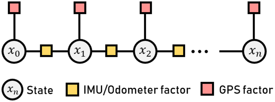
The graph structure of the proposed method is shown in Figure 3. The circle denotes the variable node, which is generated every time a new GPS measurement is available. The rectangle represents the factor node, which is derived from the measurement. The edge can exist between the variable node and factor node when the factor involves the variable. The IMU/odometer factor constrains two consecutive states by preintegration. For a GPS measurement, its factor constrains one state since it is observed at one instant.

Figure 3. Graph structure of the proposed method

The state vector in the proposed method is designed as

(25)\begin{equation} \begin{aligned} X & = [ {{x_0},{x_1}, \ldots ,{x_n}} ]\\ {x_k} & = [ {p_{{b_k}}^{w},v_{{b_k}}^{w},q_{{b_k}}^{w},{b_{{a_k}}},{b_{{w_k}}},{s_{{o_k}}},p_{{o_k}}^{{b_k}},q_{{o_k}}^{{b_k}}} ],\quad k \in[ {0,n}] \end{aligned} \end{equation}

where $X$ stands for the states set and ${x_k}$ represents the state at instant ${t_k}$, which includes the position, velocity, rotation, accelerometer bias, gyroscope bias, scale factor, and misalignments in position and attitude. Here, $n$ denotes the number of states in the sliding window.

According to Equation (21), the residual of the IMU/odometer preintegration is given by

(26)\begin{equation} r_{\textrm{I/O}}( {\hat z_{{b_{k + 1}}}^{{b_k}},X} ) = \left[ \begin{array}{c} {R_w^{{b_k}}( {p_{{b_{k + 1}}}^{w} - p_{{b_k}}^{w} - v_{{b_k}}^{w}\Delta {t_k} + \dfrac{1}{2}{g^{w}}\Delta t_k^{2}} ) - \hat \alpha_{{b_{k + 1}}}^{{b_k}}}\\ {2{{[ {{{( {\hat \gamma_{{b_{k + 1}}}^{{b_k}}})}^{ - 1}} \otimes {{( {q_{{b_k}}^{w}} )}^{ - 1}} \otimes q_{{b_{k + 1}}}^{w}} ]}_{xyz}}}\\ {R_w^{{b_k}}( {v_{{b_{k + 1}}}^{w} - v_{{b_k}}^{w} + {g^{w}}\Delta {t_k}}) - \hat \beta_{{b_{k + 1}}}^{{b_k}}}\\ {{b_{{a_{k + 1}}}} - {b_{{a_k}}}}\\ {{b_{{w_{k + 1}}}} - {b_{{w_k}}}}\\ {( {R_w^{{b_k}}p_{{b_{k + 1}}}^{w} - R_w^{{b_k}}p_{{b_k}}^{w} + R_w^{{b_k}}R_{{b_{k + 1}}}^{w}p_{{o_{k + 1}}}^{{b_{k + 1}}} - p_{{o_k}}^{{b_k}}} ) - \hat \eta_{{b_{k + 1}}}^{{b_k}}}\\ {{s_{{o_{k + 1}}}} - {s_{{o_k}}}}\\ {p_{{o_{k + 1}}}^{{b_{k + 1}}} - p_{{o_k}}^{{b_k}}}\\ {2{{[ {{{( {q_{{o_k}}^{{b_k}}} )}^{ - 1}} \otimes q_{{o_{k + 1}}}^{{b_{k + 1}}}}]}_{xyz}}} \end{array} \right] \end{equation}

The residual of the GPS measurements is formulated as

(27)\begin{align} {r_{\textrm{GPS}}}( {{{\hat z}_{\textrm{GPS}}},X} ) & = z_k^{\textrm{GPS}} - h_k^{\textrm{GPS}}( X )\nonumber\\ & = p_{{b_k}}^{\textrm{GPS}} - p_{{b_k}}^{w} \end{align}

where $z_k^{\textrm {GPS}}$ stands for the observation information at instant ${t_k}$ from the GPS receiver; $h_k^{\textrm {GPS}}( X )$ represents the observation model; and $p_{{b_k}}^{\textrm {GPS}}$ and $p_{{b_k}}^{w}$ represent the position of the GPS receiver and state, respectively.

Based on the residual of the IMU/odometer preintegration and GPS, the error function of the proposed method can be formulated as

(28)\begin{equation} \min_X \left\{ {{{\| {{r_P} - {H_P}X} \|}^{2}} + \sum_{k - n}^{k} {\| {{r_{\textrm{I/O}}}( {\hat z_{{b_{k + 1}}}^{{b_k}},X} )} \|_{P_{{b_{k + 1}}}^{{b_k}}}^{2}} + \sum_{k - n}^{k} {\| {{r_{\textrm{GPS}}}( {{{\hat z}_{\textrm{GPS}}},X} )} \|_{{P_G}}^{2}} } \right\} \end{equation}

where ${\| {{r_P} - {H_P}X} \|^{2}}$ is the prior information from marginalisation. The lower and upper limit of the summation denote the instant ${t_{k - n}}$ and instant ${t_k}$, respectively. Ceres Solver is used for solving Equation (28).

5 Experimental results

Dataset and experimental tests are executed to evaluate the performance of the proposed method compared with the Kalman filter based calibration method of Li et al. (Reference Li, Sun, Yang, Ding, Wang, Jiang, Pu, Ren, Hu and Guo2018). The graph optimisation formulated in this paper is a sliding window graph optimisation in which only past and current measurements are used, thus it can be compared with the Kalman filter under such a condition. Meanwhile, the positioning accuracy of the IMU and odometer fusion using parameters obtained from the proposed method is compared with those which employ parameters given by the preintegration models mentioned by Liu et al. (Reference Liu, Gao and Hu2019) and Chang et al. (Reference Chang, Niu and Liu2020).

5.1 Dataset results

Raw data from the KITTI dataset is first implemented to validate the effectiveness of the proposed calibration method. The KITTI datasets provide the angular rate and acceleration from IMU measurements, and the position and velocity from GPS measurements. The scale factor and misalignments in attitude and position are manually applied into the raw data to simulate the odometer and misaligned IMU measurements.

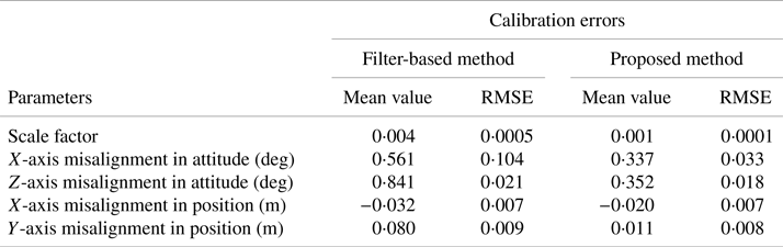
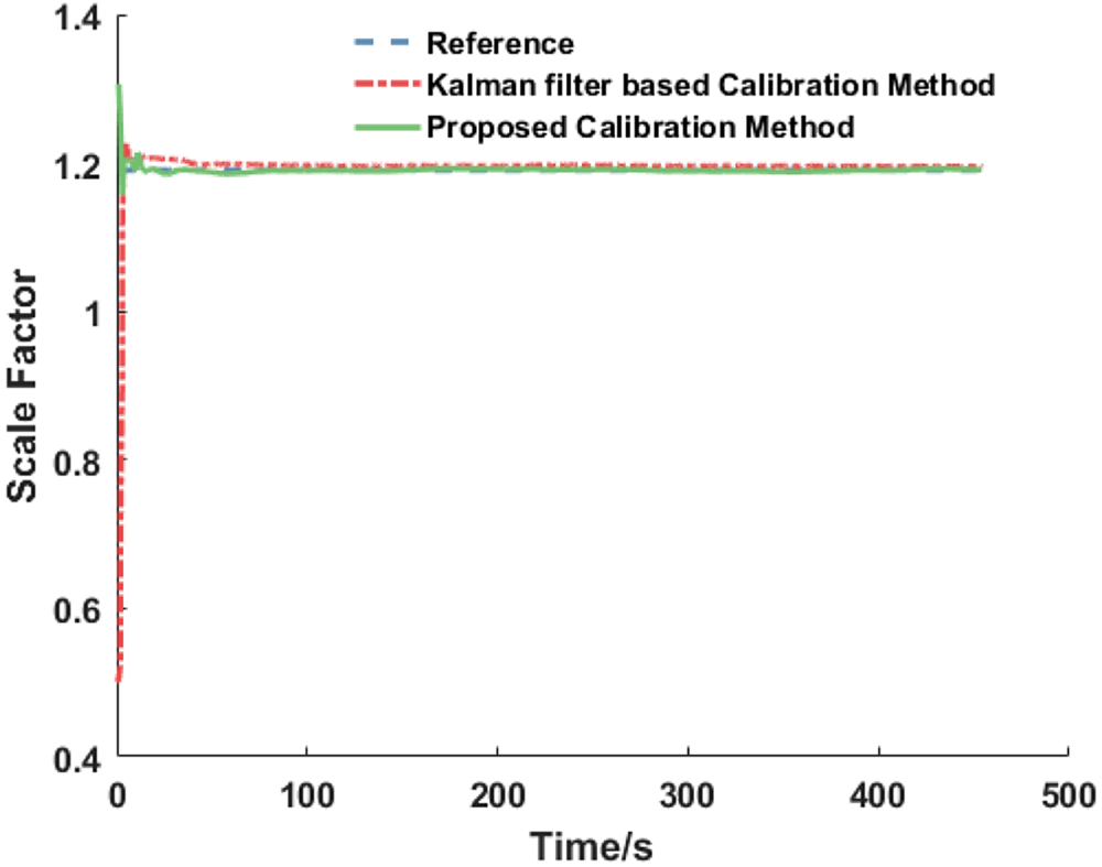
The manoeuvres of the vehicle in the KITTI dataset involves turning, accelerating and decelerating. According to the observability analysis of Liu et al. (Reference Liu, El-Sheimy and Qin2016), odometer scale factor, $x$-axis and $z$-axis misalignments in attitude, and $x$-axis and $y$-axis misalignments in position are observable. Thus, the estimation results of the above parameters are compared. Monte Carlo simulations are performed 50 times for the simulation, and the mean value and root-mean-square error (RMSE) of 50 simulations are listed in Table 2. The specific setup of the simulation parameters in one simulation is shown in Table 3. Figures 4–6 describe the comparisons of estimation results of parameters in one simulation, the blue dotted line represents the real value which is added into the raw data, the red dot–dash line denotes the estimation result of filter-based calibration method and the green solid line stands for the estimation results of the proposed calibration method.

Table 2. Statistical results in the simulation

Table 3. Setup of simulation parameters in KITTI datasets

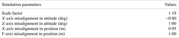
Figure 4. Comparison of scale factor of odometer

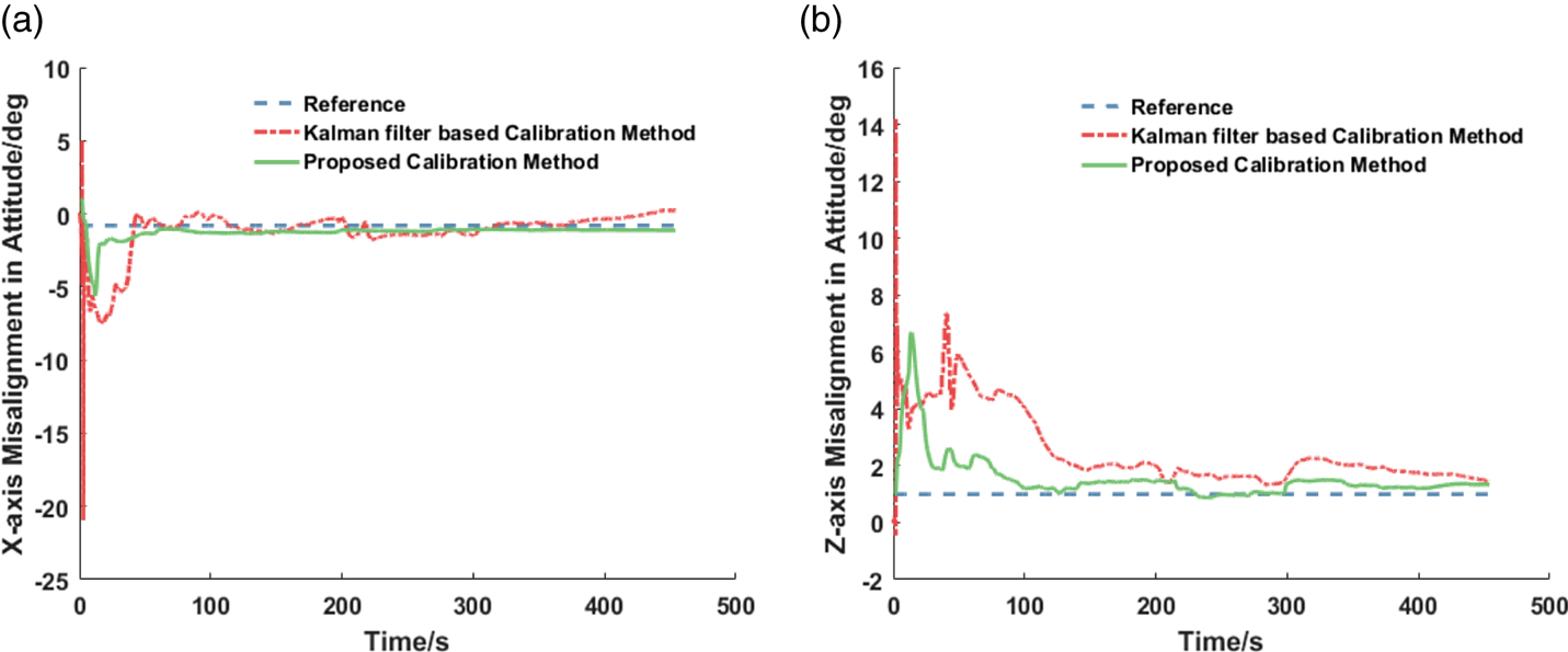
Figure 5. Comparison of misalignments in attitude: (a) $X$-axis misalignment in attitude; (b) $Z$-axis misalignment in attitude

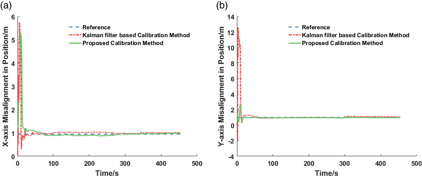
Figure 6. Comparison of misalignments in position: (a) $X$-axis misalignment in position; (b) $Y$-axis misalignment in position

From Table 2 and Figures 4–6, it could be noticed that the estimation results of the proposed method present better convergence, which are closer to the true values than the filter-based method.

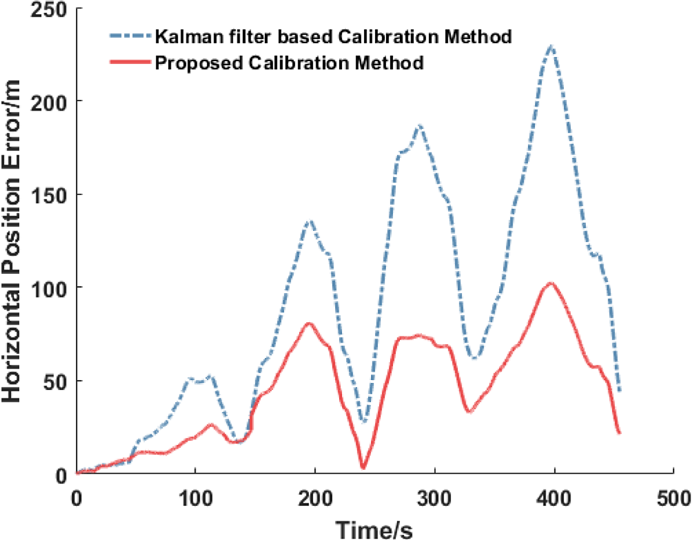
To further validate the performance of the proposed method, the mean values of the estimation results after convergence are calculated and applied into the IMU and odometer fusion. Smaller accumulative errors of the IMU and odometer fusion meant more accurate calibration results. The trajectory comparison is shown in Figure 7. It shows that the trajectory of the IMU and odometer fusion using calibration parameters from the proposed method is closer to the reference compared with the filter-based method. Figure 8 shows a comparison of the horizontal position error. The blue dot–dash line denotes the horizontal position error of the IMU and odometer fusion using calibration results of the filter-based method, and the red solid line represents the horizontal position error of the IMU and odometer fusion using calibration results of the proposed method. The latter obtained a higher positioning accuracy, which also illustrates the proposed method can achieve better calibration performance.

Figure 7. The trajectory comparison of IMU/odometer fusion using parameters given by the filter-based method and proposed method

Figure 8. The horizontal position error comparison of IMU/odometer fusion using parameters given by the filter-based method and proposed method

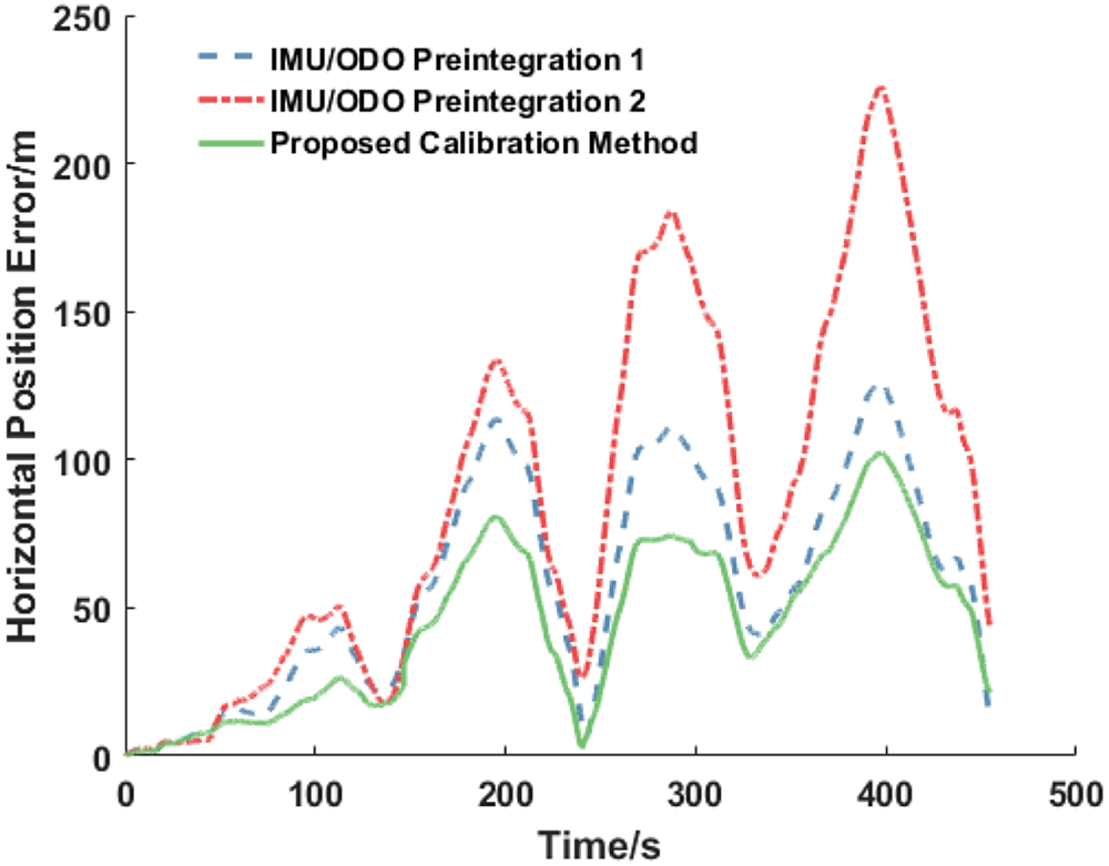
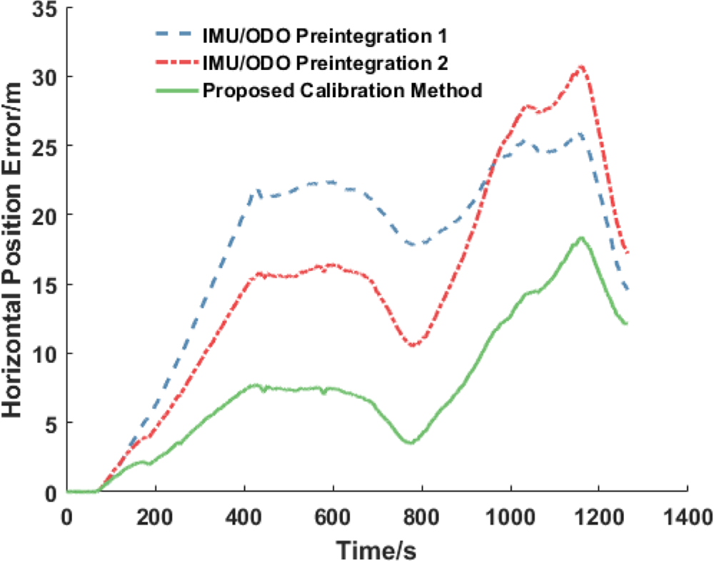
The positioning accuracy of the IMU and odometer fusion using parameters given by the preintegration models of Liu et al. (Reference Liu, Gao and Hu2019) and Chang et al. (Reference Chang, Niu and Liu2020) are also compared with the proposed method. A comparison of the trajectory is given in Figure 9 and the position error is shown in Figure 10. The blue dotted line denotes the horizontal position error of the IMU and odometer fusion using parameters from the IMU/odometer preintegration 1 mentioned by Liu et al. (Reference Liu, Gao and Hu2019) and the red dot–dash line stands for the horizontal position error using parameters from the IMU/odometer preintegration 2 mentioned by Chang et al. (Reference Chang, Niu and Liu2020). In Figure 10, the green solid line signifies the horizontal position error using parameters from the proposed method. In preintegration 1, the scale factor of the odometer is not involved in the optimisation process. The scale factor is the main source that affects the positioning accuracy of the odometer. If the scale factor is not estimated and compensated, the distance calculated by the odometer is inaccurate. In preintegration 2, misalignments in the attitude and position between the IMU and odometer are calculated by a Kalman filter and directly substituted into the preintegration. The calibration accuracy from the filter is lower than that from the graph-optimisation method. Therefore, we can see that the proposed method achieves better positioning performance.

Figure 9. The trajectory comparison of IMU/odometer fusion using parameters given by traditional preintegration methods and the proposed method

Figure 10. The horizontal position error comparison of IMU/odometer fusion using parameters given by traditional preintegration methods and the proposed method

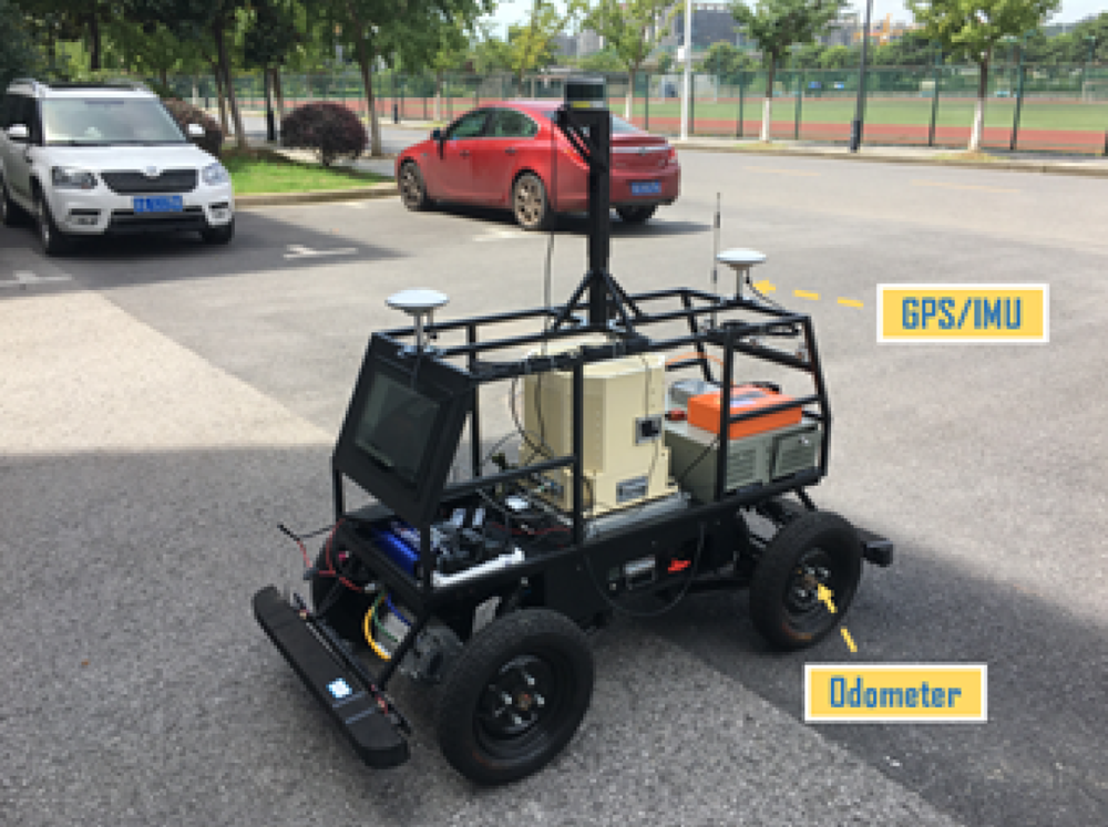
Figure 11. Baidu autonomous driving development kit

5.2 Field test results

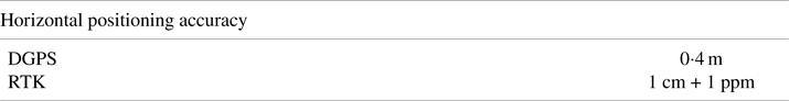
Field tests are designed to implement further evaluation of the proposed method. The test system consists of a GPS/micro-electromechanical systems (MEMS) IMU and an odometer, which are carried on a Baidu autonomous driving development kit  (Figure 11). The lever arms between the IMU and GPS have been compensated in advance. The specifications of the sensors are shown in Tables 4 and 5. In the tests, the base station service Qianxun Spatial Intelligence is used to provide a continuous RTK solution with centimetre accuracy. The GPS positioning information is collected at a rate of 1 Hz while the IMU and odometer raw measurements are logged at a sampling rate of 50 Hz. The trajectory is shown in Figure 12. In the field experimental tests, the manoeuvres of the vehicle also include turning, accelerating and decelerating, which guarantees the required parameters are observable.

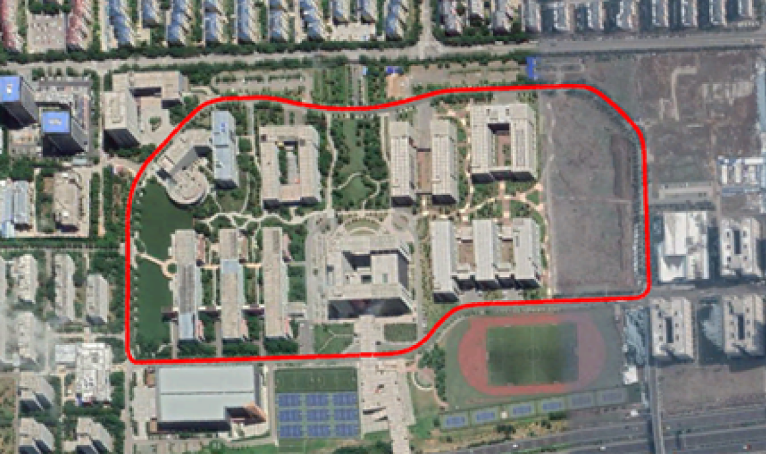
Figure 12. The trajectory of the experimental tests

Table 4. IMU sensor specifications

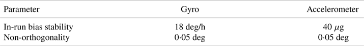
Table 5. GPS sensor specifications

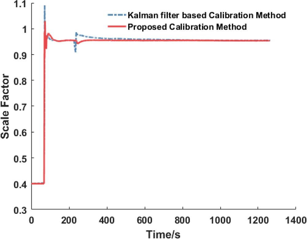
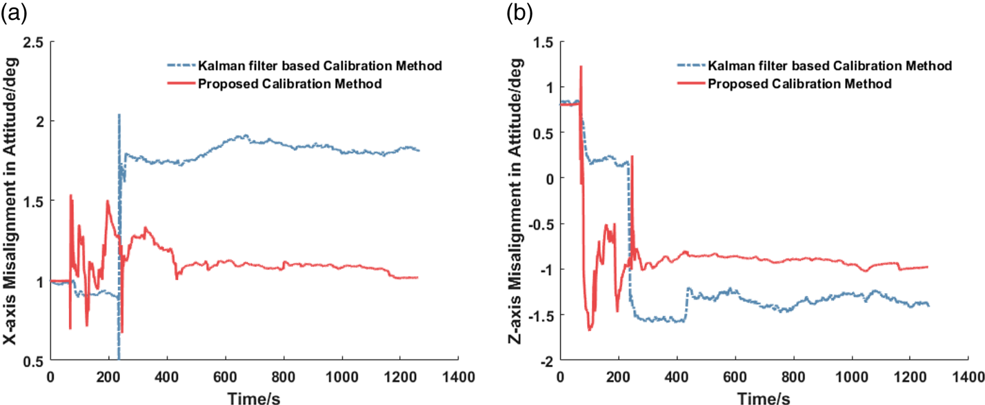
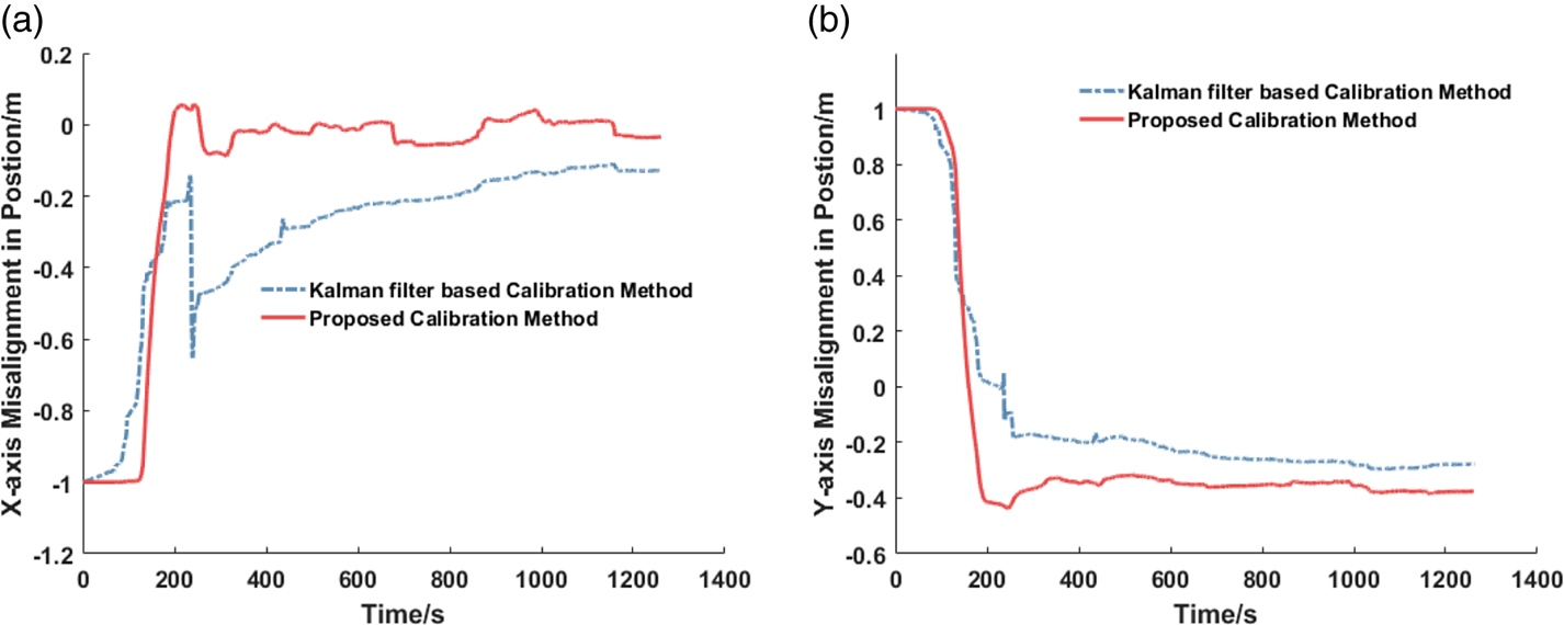
Figures 13–15 describe the comparisons of the estimation results of parameters, where the blue dot–dash line denotes the estimation results of the filter-based calibration method and the red solid line represents the estimation results of the proposed method. It could be noticed that there are larger fluctuations from 220 s to 240 s in the filter-based calibration method. This is due to the outliers of the GPS measurements. The Kalman filter estimates the states based on the measurements at the current instant and states at the last instant, which is sensitive to unexpected outliers. The proposed graph-optimisation-based calibration method takes advantage of the previous information, thus the robustness of the system is increased.

Figure 13. Comparison of scale factor of odometer

Figure 14. Comparison of misalignments in attitude: (a) $X$-axis misalignment in attitude; (b) $Z$-axis misalignment in attitude

Figure 15. Comparison of misalignments in position: (a) $X$-axis misalignment in position; (b) $Y$-axis misalignment in position

Due to the lack of reference of parameters in the experimental tests, the positioning performance of the IMU and odometer fusion is analysed. The estimation results from different methods are applied into the integrated system. Smaller accumulative errors of the IMU and odometer fusion will result in more accurate calibration results. The RTK solution serves as a reference trajectory to evaluate the position error. It can be seen from the above estimation results that the sensor parameters converge to stable ones at the end and there are little variations. Thus, the mean values of the estimation results after convergence are calculated and applied into the IMU and odometer fusion.

The comparison of the horizontal position error is given in Figure 16. The blue dot–dash line denotes the horizontal position error of the IMU and odometer fusion using calibration results of the filter-based method, and the red solid line represents the horizontal position error of the IMU and odometer fusion using calibration results of the proposed method. This indicates that the proposed method can achieve a better calibration performance.

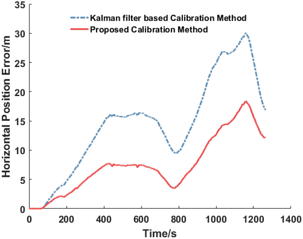
Figure 16. The horizontal position error comparison of IMU/odometer fusion using parameters given by the filter-based method and proposed method

The positioning accuracy of the IMU and odometer fusion using parameters given by preintegration1 and preintegration 2 are also compared with the proposed method, which is shown in Figure 17. The blue dotted line denotes the horizontal position error of the IMU and odometer fusion using parameters from IMU/odometer preintegration 1, the red dot–dash line stands for the horizontal position error using parameters from IMU/odometer preintegration 2 and the green solid line signifies the horizontal position error using parameters from the proposed method. The scale factor of the odometer is not considered in preintegration 1, which results in a large positioning error. In addition, the misalignments in attitude given by the Kalman filter are directly substituted into the model in preintegration 2, thereby the positioning performance is also affected. We can see that the performance of the proposed method is superior to the existing preintegrations.

Figure 17. The horizontal position error comparison of IMU/odometer fusion using parameters given by the filter-based method and proposed method