1. Introduction
By 2020, the construction of the global navigation satellite system (GNSS) gradually improved with the development of satellite navigation towards multi-frequency and multi-system (Teunissen and Montenbruck, Reference Teunissen and Montenbruck2017). Compared with GPS-only solutions, multi-GNSS solutions have more satellites and offer better spatial geometry of satellite constellation in each epoch. Such multi-systems will influence the precision and stability of the solution. Since GPS, the BeiDou navigation satellite system (BDS) and Galileo all use the code division multiple access principle, similar functional and stochastic models can be used in data processing. BDS and Galileo have been gradually built as late-stage global positioning systems (Li et al., Reference Li, Ge, Dai, Ren, Fritsche, Wickert and Schuh2015; Jin and Su, Reference Jin and Su2020). By the end of 2020, all the 30 satellites planned for BDS-3 had been launched and provided global services, including three geostationary earth orbit satellites, three inclined geosynchronous orbit satellites, and 24 medium-altitude Earth orbit (MEO) satellites (CSNO, 2019). With the successful construction of BDS-3, BDS can provide satellite observation signals with more frequency bands (Miao et al., Reference Miao, Li, Zhang and Zhang2020). The Galileo system is somewhat different from BDS. Its satellite constellation consists of three MEO planes. In theory, eight satellites are operated on each orbit plane. By the end of August 2019, the Galileo system had a total of 22 normal on-orbit working satellites in orbit (Hadas et al., Reference Hadas, Kazmierski and Sosnica2019), and by 2022 the system is planned to operate with more than 30 satellites (Yalvac, Reference Yalvac2021). In addition, all BDS and Galileo satellites can provide signals on three or more frequency bands, which greatly increases the number of observations (Li et al., Reference Li, Li, Liu, Feng, Yuan, Zhang and Ren2019). Therefore, multi-system, multi-constellation and multi-frequency signal combinations have become key application trends (Cai et al., Reference Cai, Gao, Pan and Zhu2015; Zhou et al., Reference Zhou, Dong, Li, Jiang, Wickert and Schuh2018; Li et al., Reference Li, Li, Liu, Feng, Yuan, Zhang and Ren2019).
The stochastic model reflects the statistical properties of random observation error (Li, Reference Li2016). A correct and appropriate stochastic model is essential to obtain the optimal estimator in linear models (Koch and Schönfeld, Reference Koch and Schönfeld1989). The most widely used stochastic models are based on empirical stochastic models, such as the equal-weight model, the elevation-dependent model (Eueler and Goad, Reference Eueler and Goad1991; Li et al., Reference Li, Lou and Shen2016; Xi et al., Reference Xi, Meng, Jiang, An and Chen2018), and the signal-to-noise ratio (SNR) model (Brunner et al., Reference Brunner, Hartinger and Troyer1999; Hartinger and Brunner, Reference Hartinger and Brunner1999; Wieser and Brunner, Reference Wieser and Brunner2000; Yan et al., Reference Yan, Huang, Li, Zhu, Sun, Liu, Fan and Lu2015). In the 1970s, the method of variance component estimation (VCE) in linear model was proposed (Kubik, Reference Kubik1970; Pukelsheim, Reference Pukelsheim1976). Later, some scholars proposed many variance component estimation methods, and these methods were derived under different assumptions. Commonly used variance component estimation methods include Helmert VCE (Helmert, Reference Helmert1907), least-squares variance component estimation (LS-VCE) (Pukelsheim, Reference Pukelsheim1976; Teunissen, Reference Teunissen1988; Teunissen and Amiri-Simkooei, Reference Teunissen and Amiri-Simkooei2008), minimum norm quadratic unbiased estimation (Rao, Reference Rao1971) and best invariant quadratic unbiased estimation (Schaffrin, Reference Schaffrin1981). Some scholars use this method to study the cross-correlation of GNSS observations (Teunissen, Reference Teunissen1997, Reference Teunissen, Jonkman and Tiberius1998; Bona, Reference Bona2000; Foucras et al., Reference Foucras, Leclere, Botteron, Julien, Macabiau, Farine and Ekambi2017) and study the time correlation between different epoch observations (Bona, Reference Bona2000; Hu et al., Reference Hu, Jin, Kang and Cao2018). These studies further refine the stochastic model and are used in satellite positioning processing. However, the stochastic models proposed for single-GNSS solutions are directly applied for multi-GNSS solutions under the assumption that the precision of satellites in different system constellations and observations at different frequencies are equal. The differences in the random characteristics of observations among different systems are not considered, which is unreasonable. Therefore, it is necessary to refine the stochastic model for multi-GNSS navigation and positioning.
In this paper, three refined stochastic models based on LS-VCE method are proposed to solve the problem of the observation precision uncertainties in multi-system positioning. In order to validate the proposed models in relative positioning, the relative positioning precision and ambiguity resolution success rate of zero-baseline and short-baseline were analysed compared with those of the traditional elevation-dependent model (EDM). This paper is organised as follows. In Section 2, the geometry-based multi-systems double-differenced (DD) observation model is given, including functional models and elevation-dependent stochastic models. In Section 3, the LS-VCE principle is introduced, then three refined stochastic model construction strategies based on LS-VCE are given. In Section 4, zero-baseline and short-baseline data with 8⋅19 km are processed. The impacts on single-frequency, single-epoch relative positioning precision and ambiguity resolution success rate by using different stochastic modelling strategies, i.e., EDM, RSM1, RSM2 and RSM3, are compared and analysed. Finally, some concluding remarks are made in Section 5.
2. Geometry-based observation model
2.1 GPS-BDS-Galileo functional model
In relative positioning of GNSS, the DD observation model can eliminate receiver clock errors and satellite clock errors. When the baseline distance is short (<10 km), signal propagation errors such as the ionosphere and troposphere delays are also significantly reduced (Tang et al., Reference Tang, Roberts, Hancock and Yu2018). Now suppose that two receivers are tracking satellites simultaneously; the base station and the rover station are denoted as b and r, respectively. The GPS-BDS-Galileo phase and code DD observation equation of satellite 1 and 2 can then be written as:


where the superscript * refers to different satellite navigation systems; $\phi _{br}^{12}$ and $p_{br}^{12}$
 denote the DD phase and code observations in unit of range, respectively; $\lambda$
 denotes the carrier-phase wavelength; $\rho$
 denotes the geometrical distance of satellite–receiver; ${\in}$
 and e denote the phase and code observation noise and other errors, respectively; operator $({\ast} )_{br}^{12} = ({\ast} )_b^1 - ({\ast} )_r^1 - (({\ast} )_b^2 - ({\ast} )_r^2)$
 . The clock error and atmospheric delay in the formula are both weakened and ignored here.
Since the observations suffer from inter-system bias between different systems, the reference satellites should be selected separately for each navigation system. Then, the single-frequency and single-epoch GPS-BDS-Galileo DD geometry-based linearised model can be written as:

where E(·) is the expectation operator; the superscripts g, e and c refer to GPS, Galileo and BDS system, respectively; ${\boldsymbol \phi }$ and p are phase and code DD observation vector in Equation (1) and (2); ${\boldsymbol H} ={-} {\boldsymbol e}_r^i + {\boldsymbol e}_r^j$
 and ${\boldsymbol e}_r^i$
 denotes the direction cosine vector between receiver and satellite; ${\boldsymbol \Lambda }$
 is diagonal matrix with wavelength $\lambda$
 of corresponding carrier phase; ${\boldsymbol b} = {\left[ {\begin{array}{*{20}{c}} {bx}& {by}& {bz} \end{array}} \right]^T}$
 denotes the estimated baseline coordinate vector; a denotes the DD integer ambiguities vector.
2.2 GPS-BDS-Galileo stochastic model
Among the traditional stochastic models of GNSS, the elevation-dependent stochastic model is widely used in GNSS data process. Generally, the EDM is used to describe the standard deviation (STD) of the undifferenced observations of the satellite, and the variance of DD observations can be obtained by the law of error propagation. In this paper, the traditional stochastic model is established using common trigonometric function:

where ${\sigma _0}$ is the STD of the phase or code undifferenced observations, the phase and code observation STD is set to 0⋅003 m and 0⋅3 m, respectively; $\sigma _i^2$
 is the variance corresponding to the undifferenced observation of satellite i; θ is the elevation angle of the satellite.
Therefore, the variance of undifferenced observations for each satellite can be calculated using Equation (4). The covariance matrix of the DD phase observation reads:

where the superscript ${\ast}$ denotes the different satellite systems; n is the number of visible satellites; D is the differencing matrix and ${\boldsymbol D} = [\begin{array}{*{20}{c}} { - {{\boldsymbol e}_{n - 1}}}& {{{\boldsymbol I}_{n - 1}}} \end{array}]$
 , where e is a (n–1, 1) column vector with elements that are all 1, and I is (n–1, n–1) identity matrix.
Corresponding to the observation model of Equation (3), the single-frequency GPS-BDS-Galileo DD observation stochastic model can be expressed as:

where the covariance matrix ${\boldsymbol Q}_\phi ^ \ast$ and ${\boldsymbol Q}_p^ \ast$
 are calculated using Equation (5). The superscript g, e and c refer to the GPS, Galileo and BDS systems; the subscript $\phi$
 and p denote the phase and code observation, respectively.
3. Formulation of stochastic model based on LS-VCE
LS-VCE is easy to implement because it only needs simple iteration to gain the result. This section will introduce the estimation principle of LS-VCE, then three construction strategies of three refined stochastic models based on LS-VCE are given.
3.1 LS-VCE
The linear Gauss–Markov model can be written as:

where ${{\boldsymbol Q}_0}$ is the known part of the covariance matrix, and in most cases it is a null matrix; ${\sigma _i}(i = 1,2, \ldots ,p)$
 is the unknown (co)variance components to be estimated and ${{\boldsymbol Q}_i}$
 corresponds with the known cofactor matrix. The standard least-squares solution of p variance components can solved by Equation (8) (Teunissen and Amiri-Simkooei, Reference Teunissen and Amiri-Simkooei2008):

where N is a (p, p) reversible square matrix and $\hat{{\boldsymbol \sigma }}$ and ${\boldsymbol \omega }$
 are (p, 1) vector. The elements in matrix N and ${\boldsymbol \omega }$
 can be calculated as follows (Teunissen and Amiri-Simkooei, Reference Teunissen and Amiri-Simkooei2008):


where $\hat{{\boldsymbol e}}$ is least-squares residuals, obtained as $\hat{{\boldsymbol e}}={\boldsymbol P}_A^ \bot {\boldsymbol l}$
 , with ${\boldsymbol P}_A^ \bot = {\boldsymbol I} - {\boldsymbol A}{({{\boldsymbol A}^\textrm{T}}{{\boldsymbol Q}^{ - 1}}{\boldsymbol A})^{ - 1}}{{\boldsymbol A}^\textrm{T}}{{\boldsymbol Q}^{ - 1}}$
 denoting the (m, m) orthogonal projector and m denotes number of observations; tr($\cdot$
 ) is the trace of a matrix.
Because the residuals of the phase and code DD observations of each system approximately obey zero mean normal distribution, as shown in Figure 1, the unknown variance components can be estimated using LS-VCE. Firstly, the residuals of the DD observations of GPS-BDS-Galileo can be calculated with Equation (3) and the initial value in Equation (7) can be obtained at the same time. Then the variance components can be estimated using Equation (8). The iteration continues until the convergence value of the variance components is obtained, which means that the difference between the results of two consecutive iterations is less than the tolerance:

where $||\cdot ||$ is the vector norm and δ is set to 10−6 in this paper.
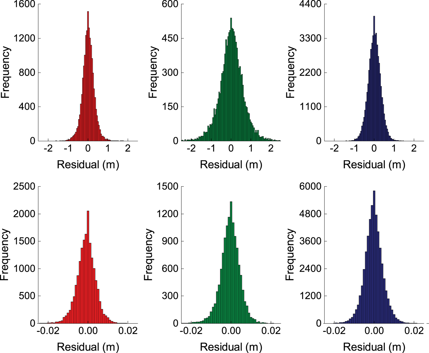
Figure 1. Residuals of DD phase (bottom) and code (top) observations on L1 (left), E1 (middle) and B1 (right)
3.2 Stochastic model refinement
If the assumptions of unknown parameters in the stochastic model are different, the estimated variance components are also different. Three different assumptions are given below (Amiri-Simkooei et al., Reference Amiri-Simkooei, Teunissen and Tiberius2009):
(1) There are differences in precision between the different systems;
(2) The precision of the phase and code observations in different frequencies is different;
(3) The precision of observations of each satellite is different.
Different refined stochastic models can then be established to solve the problem of the observation precision uncertainties in multi-system positioning.
3.2.1 Refined stochastic model 1
According to the assumption (1), the single-frequency, single-epoch stochastic model in Equation (6) can be rewritten as:

where $\sigma$ is variance components between each system, and the subscript indicates the identity of different systems. The unknown variance components vector to be estimated can be expressed as:

In order to be consistent with Equation (7), we remark the variance component elements in Equation (13) as ${\sigma _i}(i = 1,2,3)$ , where 1, 2 and 3 indicate g, e and c, respectively. The single-frequency stochastic model can then be written as:

where

Then the variance components of different systems can be estimated to construct a refined stochastic model, which is called ‘refined stochastic model 1’ (RSM1).
3.2.2 Refined stochastic model 2
According to assumption (2), different types of observations have different precision. In the case of single frequency, the variance components vector can be expressed as:

Similar to RSM1, the elements in the vector are remarked as ${\sigma _i}(i = 1,2, \ldots ,6)$ and the corresponding cofactor matrix Qi can be expressed as:

where

is the cofactor matrix of DD observations calculated by the law of error propagation, as in Equation (5).
The variance components estimated in each epoch can be applied in Equation (4) to obtain a refined stochastic model, which is called ‘refined stochastic model 2’ (RSM2).
3.2.3 Refined stochastic model 3
According to assumption (3), the observations of each satellite have different precisions. If n satellites are tracked synchronously, taking phase observations as an example, the covariance matrix of the DD observation can be expressed in the form of n variance components:

where satellite 1 is the reference satellite and its cofactor matrix is also calculated by the law of error propagation.${\sigma _i}(i = 1,2, \ldots ,n)$ denotes the variances of the undifferenced phase observations of corresponding satellites. It should be pointed out that, because the matrix N in Equation (8) is rank-deficient, the variances of the n satellites cannot be obtained in each epoch. In this case, the observations of multiple epochs are grouped for estimation.
When the variance components are estimated by using LS-VCE, the trigonometric function model can be used to fit the estimated variances components (Parkinson, Reference Parkinson1996):

where σ is the STD of undifferenced observation for phase and code in units of millimetres and metres; a 1 and a 2 are the unknown parameters that need to be fitted; θ is the satellite's elevation angle. The stochastic model obtained by fitting is called ‘refined stochastic model 3’ (RSM3), which is more realistic for the data set itself.
4. Experiments results and analysis
In this section, the traditional EDM, RSM1, RSM2 and RSM3 are used on GPS-BDS-Galileo relative positioning to analyse and evaluate the positioning precision and ambiguity resolution.
4.1 Experimental description
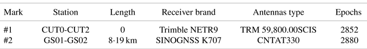
Two real GNSS data sets are used to verify the proposed stochastic model. The zero-baseline data is open source data from the Curtin GNSS Research Centre and the short-baseline data was collected in Shanghai. The zero-baseline data was collected by two Trimble NETR9 receivers and TRM 59,800⋅00 SCIS antennas on 30 June 2019. The time span of collection is 24 h with 30 s sampling interval. The short-baseline data was collected by two SINOGNSS K707 receivers and CNTAT330 antennas on 17 January 2021. The time span of collection is 24 h with 30 s sampling interval. The length of the short-baseline is 8⋅19 km and detailed information of the data sets is given in Table 1.
Table 1. Detailed information on the baseline data sets used in the experiment
4.2 Results of the zero-baseline
Because there are many ambiguity parameters in the functional model of Equation (3), the DD integer ambiguities should be fixed beforehand by LAMBDA method to obtain a simplified functional model. The different variance component parameters in RSM1 and RSM2 are estimated using Equation (8), respectively. After that, these variance components can be used to construct the RSM1 and RSM2 synchronously. In addition, the variance components of phase and code observations of each satellite are estimated to fit the parameters of RSM3.
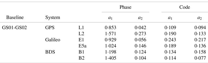
The zero-baseline data (#1) was processed in single-frequency to obtain the STD of the phase and code observations of each satellites in the experiment. Satellites with elevation angles of <10° were excluded in data processing. These STDs were then used to fit the parameters of RSM3 in Equation (19). Two frequency bands of the GPS, BDS and Galileo observations variances were estimated and fitted, respectively, being GPS (L1/L2), Galileo (E1/E5a) and BDS (B1/B2), as shown in Figure 2. The fitted parameters are shown in Table 2.
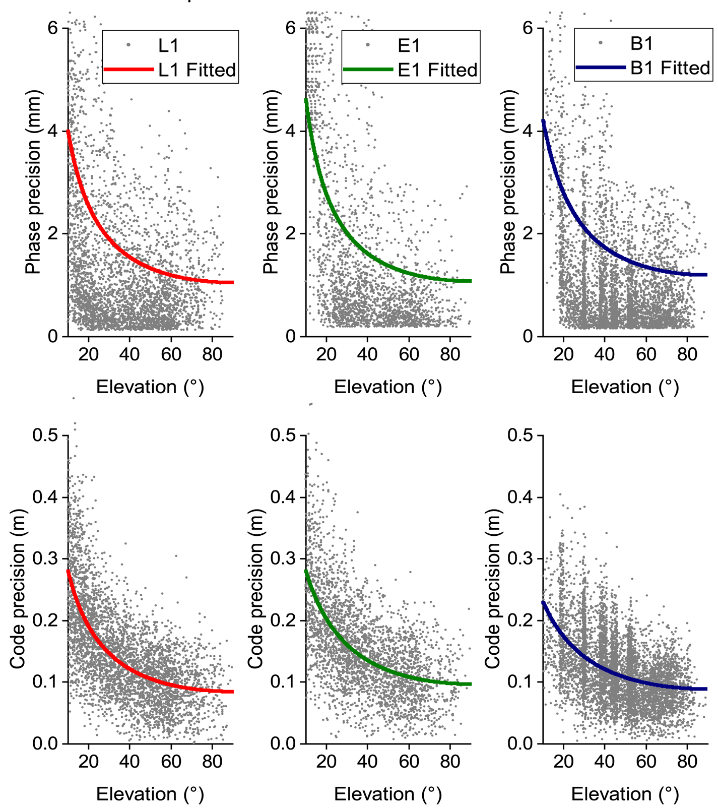
Figure 2. EDM fitted for phase (top) and code (bottom) observations on zero-baseline data (L1-B1-E1)
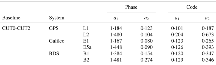
Table 2. Fitted parameters of RSM3 on zero-baseline data

In order to analyse the impact of the different stochastic models on relative positioning of the GPS-BDS-Galileo combined system, different satellite elevation mask angles were set in the experiment for single-frequency, single-epoch relative positioning. Figure 3 shows the series of the visible satellites number under different elevation mask angles of GPS-BDS-Galileo combined system.
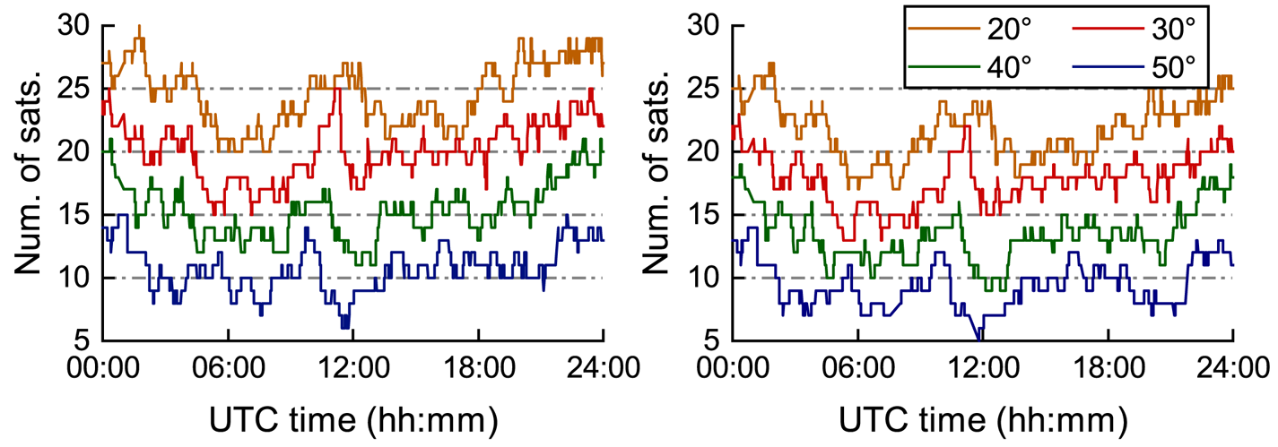
Figure 3. Numbers of visible satellites of L1-B1-E1 (left) and L2-B2-E5a (right) at different elevation mask angles
Figure 3 indicates that the average number of visible satellites at one epoch is >20 when the elevation mask angle is set to 20°, but when the elevation mask angle is set to 50°, the visible satellites in some epochs only reach about five. However, there are more visible satellites in the L1-B1-E1 frequency than in the L2-B2-E5a frequency at the same elevation mask angle because some BDS-3 satellites only provide observations in the B1 frequency. In order to ensure the stability of the variance component estimation, the maximum elevation mask angle in this paper is set to 50°.
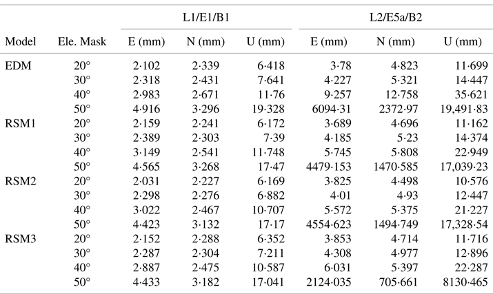
The EDM, RSM1, RSM2 and RSM3 are applied to the single-frequency, single-epoch GPS-BDS-Galileo relative positioning using zero-baseline data, and the elevation mask angles are set to 20°, 30°, 40° and 50°, respectively. Since the true value of the zero-baseline is known, the RMSE can be calculated, and the RMSE of East (E), North (N) and Up (U) component is given in Table 3.
Table 3. Calculated RMSE of zero-baseline components on L1-B1-E1 frequency and L2-B2-E5a frequency

Table 3 shows that RSM1, RSM2 and RSM3 have better performance in single-frequency, single-epoch relative positioning precision than that of EDM in most cases. However, the precision in N and U components obtained from RSM1 can be even worse than that of EDM in elevation mask of 20°. The models on the L1-B1-E1 frequency have a better performance in relative positioning than that of the L2-B2-E5a frequency because there are more visible satellites in the L1-B1-E1 frequency under the same elevation mask angle, as shown in Figure 3. It is worth noting that the relative positioning precision is significantly reduced when the elevation mask angle is set to 50° because of the small number of visible satellites in the combined system. RSM3 has the best performance in zero-baseline solutions. Figure 4 depicts the precision improvements in percentage brought by RSM1, RSM2 and RSM3 when compared with EDM.

Figure 4. Relative positioning precision improvement in percentage, comparing RSM1 (left), RSM2 (middle) and RSM3 (right) with EDM, for L1-B1-E1 (top) and L2-B2-E5a (bottom)
Figure 4 indicates that, compared with the EDM, the precision of RSM3 has been improved obviously, especially when the elevation mask angle is set to 50°. As for RSM1, the precision on L1-B1-E1 is nearly the same as that of EDM, and sometimes deterioration occurs (within 2%) on N and U components when the elevation mask is set to 20°. When the elevation mask angle ≥40°, there are significant improvements in all three directions on L2-B2-E5a frequency. RSM2 performs better when the elevation mask angle ≤40°, however the precision on L1-B1-E1 frequency shows no improvement when there are fewer satellites that can be tracked on a 50° elevation mask angle. RSM3 performs the best among the three refined stochastic models, and the precision can be improved 4⋅6%, 7⋅6%, 13⋅2%, 73⋅0% for L1-B1-E1, and 1⋅1%, 4⋅8%, 16⋅3%, 64⋅5% for L2-B2-E5a at 20°, 30°, 40°, 50° elevation mask angles, respectively.
As is known, the resolution of the DD integer ambiguity is a key step in high-precision relative positioning (Amiri-Simkooei et al., Reference Amiri-Simkooei, Jazaeri, Zangeneh-Nejad and Asgari2016). The ambiguity resolution success rate (SR) is an important indicator to evaluate the quality of the baseline solution. Figure 5 gives the single-frequency, single-epoch ambiguity resolution SR for different stochastic models in the cases of different elevation mask angles.

Figure 5. SR of four stochastic models on L1-B1-E1 (top) and L2-B2-E5a (button) for different elevation mask angles
Figure 5 shows that the four stochastic models have almost the same performance in ambiguity resolution SR of the zero-baseline. The impact of the decrease in the number of visible satellites caused by the increase in the elevation mask angle on SR is more significant. The SR of the L1-B1-E1 frequency is close to 100%, and the SR is still greater than 90% even when the elevation mask angle is set to 50°. The SR in the L2-B2-E5a frequency gradually drops to about 70% due to the relatively small number of satellites.
4.3 Results of the short-baseline
The short-baseline data (#2) collected by SINO K707 receivers was processed and analysed. Similarly, the variances of each satellite observations are estimated beforehand to fit the parameters in RMS3. The results and fitted paraments are shown in Figure 6 and Table 4, respectively.
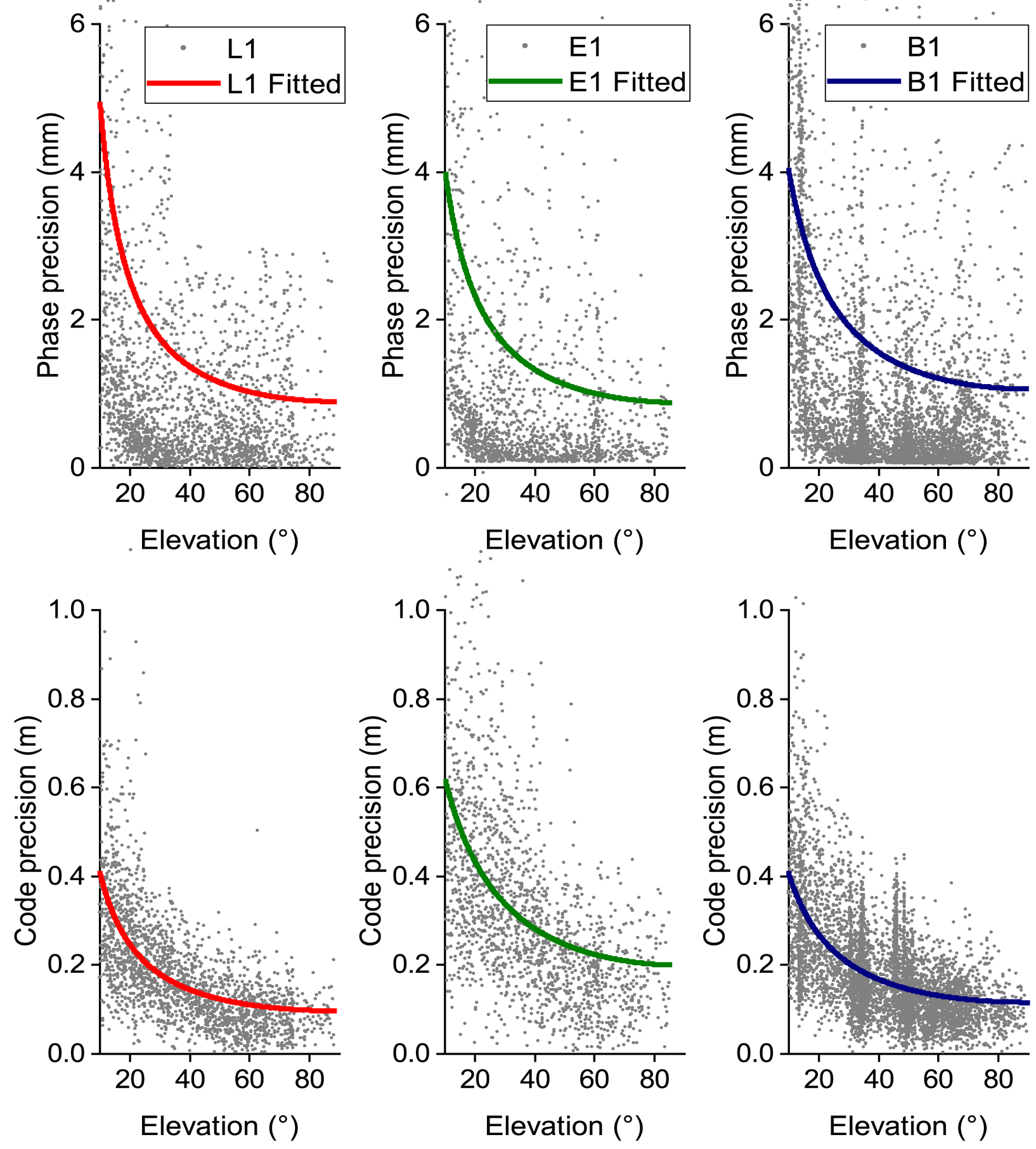
Figure 6. EDM fitted for phase (top) and code (bottom) observations on short-baseline data (L1-B1-E1)
Table 4. Fitted parameters of RSM3 on short-baseline data

The four stochastic models were also applied to the short-baseline data processing. The experiment was also set up at the satellite elevation mask angles of 20°, 30°, 40° and 50°, respectively. Figure 7 shows the series of the number of visible satellites under different elevation mask angles. It can be seen that, similar to zero-baseline, the number of visible satellites in the L1-B1-E1 frequency is still significantly greater than that in the L2-B2-E5a frequency because not all B2 signals of BDS can be tracked.
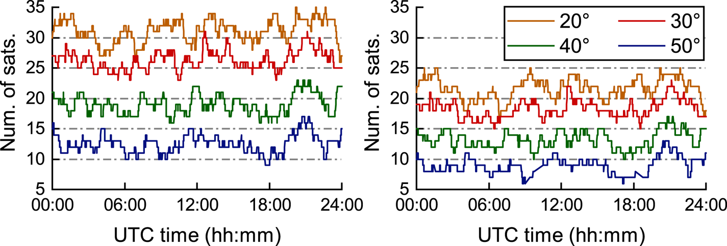
Figure 7. Numbers of visible satellites of L1-B1-E1 (left) and L2-B2-E5a (right) at different elevation mask angles
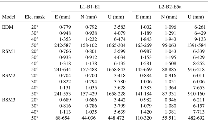
The STD of baseline components in E, N and U is calculated using four stochastic models, and the results are given in Table 5. It can be seen in Table 5 that the L1-B1-E1 frequency had better performance in relative positioning precision than the L2-B2-E5a frequency. Especially when the elevation mask angle is 50°, the L1-B1-E1 frequency can still maintain a relatively stable positioning precision with the help of the successful construction of the BDS-3.
Table 5. Calculated STD of short-baseline components on L1-B1-E1 frequency and L2-B2-E5a frequency
The precision improvements in percentage brought by RSM1, RSM2 and RSM3 when compared with EDM are shown in Figure 8. Figure 8 shows that the precision improvement of RSM1, RSM2 and RSM3 on the L1-B1-E1 frequency is not obvious compared with the L2-B2-E5a frequency, and the precision improvement on L1-B1-E1 frequency is below 10%. In contrast, the precision of the short-baseline solution on L2-B2-E5a frequency is improved by at least 20% when fewer than 15 satellites can be tracked on elevation mask angle ≥40°. Moreover, the precision of L2-B2-E5a frequency is improved more significantly than on L1-B1-E1 frequency when the elevation mask angle ≥40°. RSM3 performs best among the four stochastic models, and the precision at 20°, 30°, 40°, 50° elevation mask angles can be improved 0⋅9%, 5⋅2%, 9⋅4%, 11⋅5% for L1-B1-E1, and 0⋅2%, 9⋅3%, 39⋅1%, 58⋅9% for L2-B2-E5a, respectively, which is consistent with the conclusion of the zero-baseline experiment.
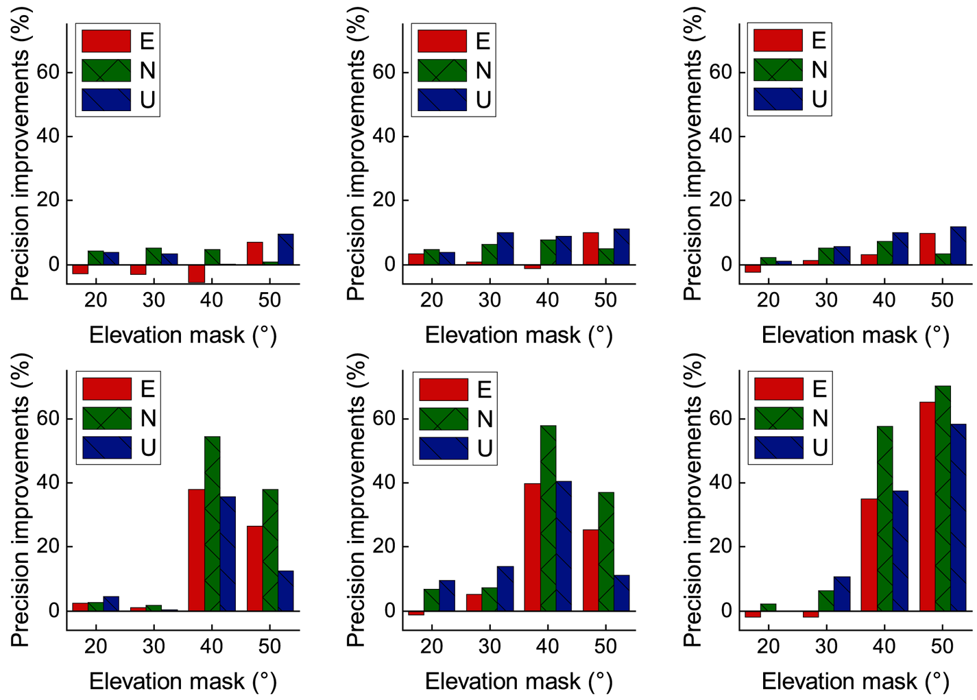
Figure 8. Relative positioning precision improvement in percentage comparing RSM1 (left), RSM2 (middle) and RSM3 (right) with EDM, for L1-B1-E1 (top) and L2-B2-E5a (bottom)
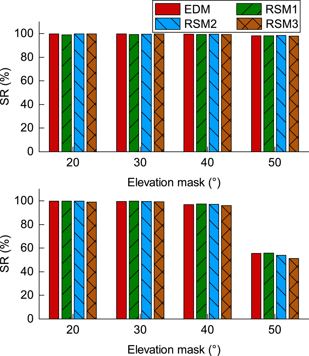
Finally, the single-frequency, single-epoch ambiguity resolution SR for different stochastic models be calculated with the whole piece of the data set (2,880 epochs), as shown in Figure 9. Figure 9 indicates that EDM, RSM1, RSM2 and RSM3 have almost the same performance in ambiguity resolution SR. Owing to the successful construction of BDS-3, the combined system on the L1-B1-E1 frequency still has >10 satellites that can be tracked even when the elevation mask angle is set to 50°. The SR of the L1-B1-E1 frequency did not decrease with the increase of the elevation mask angle. As show in Figure 7, because not all B2 signals of BDS can be tracked, the minimum number of the observations on L2-B2-E5a frequency can decrease to six. Thus, the ambiguity resolution SR on L2-B2-E5a is only about 50%, and the SR of RSM3 is slightly worse than the other three stochastic models when the elevation mask angle set to 50°.

Figure 9. SR of four stochastic models on L1-B1-E1 (top) and L2-B2-E5a (button) for different elevation mask angles
5. Conclusions
A suitable stochastic model is important for multi-GNSS navigation and positioning. However, most stochastic models proposed for single-GNSS solutions are directly applied for multi-GNSS solutions under the assumption that the precision of satellites in different system constellations and observations at different frequencies is equal. The differences in the random characteristics of observations among different systems are not considered. In this paper, three refined stochastic models, namely, RSM1, RSM2 and RSM3, based on the LS-VCE method are proposed to solve the problem of the observation precision uncertainties in multi-system positioning. A set of zero-baseline data from Curtin GNSS Research Centre and a data set of short-baseline with 8⋅19 km were used to analyse and verify the proposed stochastic models. Results of both zero-baseline and short-baseline experiments show that the proposed RSM1, RSM2 and RSM3 demonstrated better performance in relative positioning precision compared with EDM in most cases. RSM3, which is more realistic for the data itself, performs the best. The maximum improvements of relative positioning precision in elevation mask angles 20°, 30°, 40°, 50° were about 4⋅6%, 7⋅6%, 13⋅2%, 73⋅0% for L1-B1-E1, and 1⋅1%, 4⋅8%, 16⋅3%, 64⋅5% for L2-B2-E5a, respectively. For ambiguity resolution SR, the refined stochastic models are not significantly improved when compared with EDM, and sometimes SR is slightly reduced. Therefore, a realistic stochastic model can improve the precision of GNSS positioning, especially when fewer satellites can be tracked.
Acknowledgements
This work is sponsored by the National Natural Science Foundation of China (Nos. 41704036 and 41604028). The authors gratefully thank the Curtin GNSS Research Centre of Curtin University for providing its data sets.