2. TRIPLE-FREQUENCY CODE AND PHASE OBSERVATIONS

A linear combination between pseudo-range measurements $P_{r, 1}^{s} $, $P_{r, 2}^{s} $ and $P_{r, 3}^{s} $ on the three frequencies f ₁, f ₂ and f ₃, recorded at time t by the receiver r and transmitted by the satellite s can be written as

(1)$$\begin{aligned} P_r^s ( t ) & =\alpha _1 P_{r,1}^s ( t ) +\alpha _2 P_{r,2}^s ( t ) +\alpha _3 P_{r,3}^s ( t ) \\ & =( {\alpha_1 +\alpha_2 +\alpha_3 } ) \cdot \rho _r^s ( t ) +\left( {\alpha_1 +\alpha_2 \frac{f_1^2 }{f_2^2 }+\alpha_3 \frac{f_1^2 }{f_3^2 }} \right)\cdot I_{r,1}^s ( t ) +e_r^s ( t ) \end{aligned}$$

Similarly, a combination between three phase measurements, $L_{r, 1}^{s} $, $L_{r, 2}^{s} $ and $L_{r, 3}^{s} $, expressed in units of meters, can be expressed as

(2)$$\begin{aligned} L_r^s ( t ) & =\alpha _1 L_{r,1}^s ( t ) +\alpha _2 L_{r,2}^s ( t ) +\alpha _3 L_{r,3}^s ( t ) \\ & =( {\alpha_1 +\alpha_2 +\alpha_3 } ) \cdot \rho _r^s ( t ) -\left( {\alpha_1 +\alpha_2 \frac{f_1^2 }{f_2^2 }+\alpha_3 \frac{f_1^2 }{f_3^2 }} \right)\cdot I_{r,1}^s ( t ) -\alpha _1 \lambda _1 ( {N_{r,1}^s +d_{r,1}^s } ) \\ & \quad -\alpha _2 \lambda _2 ( {N_{r,2}^s +d_{r,2}^s } ) -\alpha _3 \lambda _3 ( {N_{r,3}^s +d_{r,3}^s } ) +\varepsilon _r^s ( t ) \end{aligned}$$

For simplicity, in Equations (1) and (2) the nondispersive term $\rho _{r}^{s} $ includes the geometric range, the receiver's and satellite's clock offsets, and the tropospheric delay. In Equation (2), the terms $N_{r, i}^{s} $ and $d_{r, i}^{s} $ represent the integer ambiguity and its fractional part (FCB), due to the receiver and satellite hardware bias, of the phase measurement on frequency f _i (with λ_i being the wavelength). The terms α₁, α₂ and α₃ are simple scalar factors of the combination. The ionospheric delay $I_{r, 1}^{s} $ affecting signals on frequency f ₁ is amplified by the term

(3)$$q=\left( {\alpha_1 +\alpha_2 \frac{f_1^2 }{f_2^2 }+\alpha_3 \frac{f_1^2 }{f_3^2 }} \right)$$

While the noises in the code and phase combinations, $e_{r}^{s} $ and $\varepsilon _{r}^{s} $, have a standard deviation

(4)$$\begin{align} \sigma _{e_r^s } & =\sqrt {\alpha _1^2 \sigma _{e_{r,1}^s }^2 +\alpha _2^2 \sigma _{e_{r,2}^s }^2 +\alpha _3^2 \sigma _{e_{r,3}^s }^2 } \notag\\ & =\sigma _{e_{r,1}^s } \sqrt {\alpha _1^2 +\alpha _2^2 n_2^2 +\alpha _3^2 n_3^2 } =n_P \cdot \sigma _{e_{r,1}^s } \end{align}$$

(5)$$\begin{align} \sigma _{\varepsilon _r^s } & =\sqrt {\alpha _1^2 \sigma _{\varepsilon _{r,1}^s }^2 +\alpha _2^2 \sigma _{\varepsilon _{r,2}^s }^2 +\alpha _3^2 \sigma _{\varepsilon _{r,3}^s }^2 } \notag\\ & =\sigma _{\varepsilon _{r,1}^s } \sqrt {\alpha _1^2 +\alpha _2^2 +\alpha _3^2 } =n_L \cdot \sigma _{\varepsilon _{r,1}^s } \end{align}$$

which are n _P and n _L times larger than the standard deviation of the error in the code and carrier phase on frequency f ₁, respectively.

For simplicity, in Equation (5), the residual carrier phases (expressed in units of meters) on different frequencies were assumed to have the same noise level. Although not formally correct, in our processing we assumed that the difference in the noise level of phase measurements on different frequencies is much smaller than other sources of error, such as residual error in the products or troposphere modelling.

In order to preserve the nondispersive term $\rho _{r}^{s} $ in the combination, the following condition must be satisfied

(6)$$\alpha _1 +\alpha _2 +\alpha _3 =1$$

Moreover, the ionosphere amplification factor q must be nullified to have an IF combination.

(7)$$\alpha _1 +\alpha _2 \frac{f_1^2 }{f_2^2 }+\alpha _3 \frac{f_1^2 }{f_3^2}=0$$

3. TRIPLE-CARRIER COMBINATIONS THAT OPTIMISE THE REDUCTION OF NOISE IN THE INTEGER AMBIGUITY

Equations (6) and (7) describe a system of two linear equations with three unknowns α₁, α₂ and α₃. Using the third frequency gives the solution space one degree of freedom that can be exploited to impose one more constraint to the combination, for example reducing the noise. Since Deo and El-Mowafy (Reference Deo and El-Mowafy2016) already proved that triple-frequency combinations with minimum noise do not bring large improvements to the PPP convergence time, this type of constraint is not considered here. Instead, this research tests triple-frequency combinations that optimise the noise of the NL ambiguity observable (Basile et al., Reference Basile, Moore, Hill and Mcgraw2018a).

By rewriting the ambiguity terms in Equation (2) as a combination between the EWL $( N_{r, ew}^{s} =N_{r, 3}^{s} -N_{r, 2}^{s} ) $, WL $( N_{r, w}^{s} =N_{r, 2}^{s} -N_{r, 1}^{s} ) $ and NL $( N_{r, n}^{s} =N_{r, 1}^{s} ) $ ambiguities

(8)$$\begin{align} \alpha _1 \lambda _1 N_{r,1}^s +\alpha _2 \lambda _2 N_{r,2}^s +\alpha _3 \lambda _3 N_{r,3}^s &=\alpha _3 \lambda _3 N_{r,ew}^s +( {\alpha_2 \lambda_2 +\alpha_3 \lambda_3 } ) N_{r,w}^s\notag\\ &\quad +( {\alpha_1 \lambda_1 +\alpha_2 \lambda_2 +\alpha_3 \lambda_3 } ) N_{r,n}^s \end{align}$$

it can be demonstrated that for a given pseudo-range noise level (with variance $\sigma _{e_{r}^{s} }^{2} ) $ there exist a triple-carrier IF combination that reduces the noise in the NL ambiguity observable:

(9)$$\begin{align} N_{r,n}^s &=\frac{P_{r,IF}^s -L_{r,IF}^s }{( {\alpha_1 \lambda_1 +\alpha_2 \lambda_2 +\alpha_3 \lambda_3 } ) } \end{align}$$

(10)$$\begin{align} \sigma _{N_{r,n}^s }^2 &=\frac{\sigma _{e_r^s }^2 +\sigma _{\varepsilon _r^s }^2 }{( {\alpha_1 \lambda_1 +\alpha_2 \lambda_2 +\alpha_3 \lambda_3 } ) ^2} \end{align}$$

Figure 1 shows the error in the NL ambiguity observable as a function of the amplified NL wavelength for the GPS triple-frequency IF combination. Here, the error in the pseudo-ranges on L1 and L5 were assumed to be equal to 1 m and 0·8 m, respectively, while the carrier phase measurements were assumed to have a precision of 1 cm. This figure was generated by making the amplified NL wavelength vary between 0·1 m and 1·7 m, with a step-size of 0·01 m; and computing the corresponding NL ambiguity noise value. It can be seen that the error in the NL ambiguity observable has a minimum corresponding to an amplified NL wavelength of 0·66 m.

Figure 1. Noise in the narrow-lane ambiguity observable as a function of the amplified NL wavelength. GPS L1-L2-L5 IF combinations.

The coefficients α₁, α₂ and α₃ corresponding to the minimum error level of the NL ambiguity observable can be analytically computed by solving Equations (6), (7) and (11):

(11)$$\frac{\partial \sigma _{N_{r,n}^s }^2 }{\partial \alpha _3 }=0$$

From Equations (6) and (7), we can write

(12)$$\begin{cases} \alpha_1 =-\dfrac{q_2 }{1-q_2 }+\dfrac{q_2 -q_3 }{1-q_2 }\alpha _3 =A+B\alpha _3 \\ \alpha _2 =\dfrac{1}{1-q_2 }-\dfrac{1-q_3 }{1-q_2 }\alpha _3 =C+D\alpha _3 \end{cases}$$

Replacing Equation (12) into Equation (10)

(13)$$\sigma _{N_{r,n}^s }^2 =\frac{\sigma _{e_r^s }^2 +\sigma _{\varepsilon _r^s }^2 }{[ {( {A\lambda_1 +C\lambda_2 } ) +( {B\lambda_1 +D\lambda_2 +\lambda_3 } ) \cdot \alpha_3 } ] ^2}=\frac{\sigma _{e_r^s }^2 +\sigma _{\varepsilon _r^s }^2 }{[ {E+F\cdot \alpha_3 } ] ^2}$$

where

(14)$$ \sigma _{\varepsilon _r^s }^2 =\sigma _{\varepsilon _{r,1}^s }^2 [ {( {A+B\alpha_3 } )^2+( {C+D\alpha_3 } )^2+\alpha_3^2 } ] $$

the solution of Equations (6), (7) and (11), by taking into account Equations (12), (13) and (14), is

(15)$$\begin{cases} {\alpha _1 =A+B\alpha _3 } \\ {\alpha _2 =C+D\alpha _3 } \\ {\alpha _3 =\dfrac{\sigma _{\varepsilon _{r,1}^s }^2 [ {F( {A^2+C^2} ) -E( {AB+CD} ) } ] +\sigma _{e_r^s }^2 \cdot F}{\sigma _{\varepsilon _{r,1}^s }^2 [ {E( {B^2+D^2+1} ) -F( {AB+CD} ) } ] }} \end{cases}$$

These triple-carrier IF combinations with larger NL wavelength enhance the observability of the NL ambiguities; hence, one would expect some improvement in the convergence time of the float PPP solution. Unfortunately, using these combinations alone is not very effective since they are characterised by a large noise level. Figure 2 compares the noise in the NL ambiguity observable and the noise in the corresponding triple-carrier IF combination for different amplified NL wavelengths. The IF combination that provides the best observability of the NL ambiguity has a noise 557·4 times larger than the error in the single carrier phase measurement. Assuming, for severe multipath environments, a carrier phase with an accuracy of 1 cm, the proposed IF combination has a noise level of 5·57 m.

Figure 2. Noise in the narrow-lane ambiguity observable (blue plot with y-axis on the left) and amplification factor of the corresponding triple-carrier IF combination (red plot with y-axis on the right) as a function of the amplified NL wavelength. GPS L1-L2-L5 IF combinations.

For this reason, the triple-carrier combination that minimise the error in the NL observable will be coupled with the traditional dual-frequency IF combination. In this way, while the first combination speeds up the convergence time in PPP, the second one is useful to keep the final accuracy to centimetres-level.

In order to make this algorithm work, it is necessary that the two IF carrier phase combinations are affected by the same ambiguity value. Hence, the EWL and WL ambiguities have to be fixed, and the FCBs must be corrected for.

4. EXTRA-WIDE-LANE AND WIDE-LANE AMBIGUITY FIXING

In carrier phase-based positioning techniques exploiting two-frequency IF combinations, an ambiguity fixed solution can be obtained only after the WL ambiguity $N_{r, w}^{s} $ is fixed. Traditionally, the Melbourne–Wubbena combination $L_{r, m}^{s} $ (Melbourne, Reference Melbourne1985; Wubbena, Reference Wubbena1985), between pseudo-ranges $P_{r, 1}^{s} $ and $P_{r, 2}^{s} $, and carrier phases $L_{r, 1}^{s} $ and $L_{r, 2}^{s} $ on frequency f ₁ and f ₂, is adopted for this purpose:

(16)$$L_{r,m}^s =\frac{f_1 P_{r,1}^s +f_2 P_{r,2}^s }{f_1 +f_2 }-\frac{f_1 L_{r,1}^s -f_2 L_{r,2}^s }{f_1 -f_2 }=-\lambda _w ( {N_{r,w}^s +d_{r,m}^s } ) $$

In Equation (16), $d_{r, m}^{s} $ is the FCB in the combination due to satellite and receiver hardware. While the satellite FCB can be computed in a network solution and disseminated together with the precise PPP products, the receiver part can be removed by single differentiation between satellites.

As an alternative, Geng and Bock (Reference Geng and Bock2013) proposed an algorithm based on a triple-frequency combination that guarantees an improved WL ambiguity fix success rate with respect to the one achievable with $L_{r, m}^{s} $. In the first step, measurements on L2 and L5 frequency are combined into the Melbourne–Wubbena combination $L_{r, em}^{s} $ with the aim to fix the EWL ambiguity $N_{r, ew}^{s} $:

(17)$$L_{r,em}^s =\frac{f_2 P_{r,2}^s +f_5 P_{r,5}^s }{f_2 +f_5 }-\frac{f_2 L_{r,2}^s -f_5 L_{r,5}^s }{f_2 -f_5 }=-\lambda _{ew} ( {N_{r,ew}^s +d_{r,em}^s } ) $$

The EWL wavelength λ_ew is so large (about 5·86 m) that it makes the instantaneous ambiguity resolution success rate more than 99·9%. As per (14), $d_{r, em}^{s} $ in the combination Equation (17) can be mitigated by the FCBs corrections computed in the network solution.

In the second step, the WL ambiguity is estimated using the IF combinations between pseudo-ranges on L1 and L2 $( P_{r, IF}^{s} ) $, and between the WL and the unambiguous EWL carrier combinations $( L_{r, x}^{s} ) $:

(18)$$\begin{align} P_{r,IF}^s &=\frac{f_1^2 }{f_1^2 -f_2^2 }P_{r,1}^s -\frac{f_2^2 }{f_1^2 -f_2^2 }P_{r,2}^s \end{align}$$

(19)$$\begin{align} L_{r,x}^s &=\frac{f_1 }{f_1 -f_5 }L_{r,w}^s -\frac{f_5 }{f_1 -f_5 }( {L_{r,ew}^s -\lambda_{ew} {N}''} ) \end{align}$$

with

(20)$$\begin{align} L_{r,ew}^s &=\lambda _{ew} \left( {\frac{L_{r,2}^s }{\lambda_2 }-\frac{L_{r,5}^s }{\lambda_5 }} \right) \end{align}$$

(21)$$\begin{align} L_{r,w}^s &=\lambda _w \left( {\frac{L_{r,1}^s }{\lambda_1 }-\frac{L_{r,2}^s }{\lambda_2 }} \right) \end{align}$$

In Equation (19), $d_{r, x}^{s} $ denotes the hardware bias in $L_{r, x}^{s} $ that have to be corrected to have an integer WL ambiguity $N_{r, w}^{s} $.

Even though the noisy $P_{r, IF}^{s} $ is used as the base pseudo-range and the noise on $L_{r, x}^{s} $ is roughly 110 times larger than the carrier phase error, the WL wavelength is amplified to 3·40 m, which is large enough to reliably fix the WL ambiguity to its nearest integer value in just a few epochs. Being a geometry-free algorithm, the time required to fix the WL ambiguity depends on two factors: the quality of the measurements and the multipath correlation time constant. Indeed, one would expect longer times to achieve an ambiguity resolution correct-fix rate over 99·9% if the errors in the measurements adopted as base pseudo-range to fix the WL ambiguity are large or highly time correlated.

The dependence of the time to first ambiguity fix on the measurements error and correlation time was proved through simulated data. Details regarding the simulator can be found in Basile et al. (Reference Basile, Moore and Hill2019). Figure 3 compares the correct-fix rate of the WL ambiguity resolution when the simulated measurements are recorded in a benign environment and when the receiver is located in a multipath-rich site. In order to simulate the multipath for a given measurement, the correlation time constant was obtained from a generator of normally distributed variables with mean equal to 35 s and standard deviation equal to 10 s. In this way, the multipath correlation time constant lies for 99% of the time in the range between 5 and 65 s (Khanafseh et al., Reference Khanafseh, Kujur, Joerger, Walter, Pullen, Blanch, Doherty, Norman, De Groot and Pervan2018). Observations spanning more than 4 h were divided into short sessions of t seconds, and WL ambiguity resolution was carried out at the last epoch of each session. The correct-fix rate is computed as the ratio between the numbers of t-second sessions with correct ambiguity resolution and the number of all t-seconds epochs. The same approach was used in Geng and Bock (Reference Geng and Bock2013) to prove the benefit of Triple-Carrier Ambiguity Resolution (TCAR) over dual-frequency ambiguity resolution. In absence of multipath, the WL ambiguity for GPS can be fixed in only 2 s, while users have to wait for as long as 14 min when the GPS pseudo-ranges and carrier phase measurements are affected by multipath. Similarly, the ambiguity in Galileo carrier phase WL combinations can be instantaneously fixed for a multipath-free site, but in 9 min if the measurements have poor quality.

Figure 3. Wide-lane ambiguity correct-fix rate for GPS L1-L2-L5 (blue) and Galileo E1-E5-E6 (red) combinations for a benign environment (left) and multipath-rich site (right).

Also, the effect of different multipath correlation time constants on the WL ambiguity correct-fix rate was tested. For this purpose, a new simulation scenario was configured in which all the GNSS measurements were assumed to be affected by multipath with the same correlation time constant, from 2 to 60 s. The time required to have the WL ambiguity fixed greatly increases with the multipath correlation time constants. As shown in Figure 4, for a multipath correlation time of 10 s, the GPS and Galileo WL ambiguities can be fixed in 4·5 min and 3·5 min, respectively, but with a correlation time of 60 s users have to wait for more than 20 min to fix the WL ambiguities following the method presented in Geng and Bock (Reference Geng and Bock2013).

Figure 4. Sensitivity of the wide-lane ambiguity fix time to the multipath correlation time constant.

In this paper, a different approach is presented. Instead of using the traditional IF pseudo-range combination as a base pseudo-range to fix the WL ambiguity, a low-noise pseudo-range combination corrected by the smoothed ionosphere correction is employed. Basile et al. (Reference Basile, Moore, Hill, Mcgraw and Johnson2018b, Reference Basile, Moore, Hill, Mcgraw and Johnson2018c, Reference Basile, Moore and Hill2019) adopted the smoothed ionosphere corrected pseudo-range combinations to reduce the reconvergence time of PPP and, consequently, improve the positioning solution in urban environments. Basile et al. (Reference Basile, Moore, Hill and Mcgraw2018a), instead, exploited these combinations to improve the NL ambiguity correct-fix rate.

The noise in the triple frequency pseudo-range combination, as defined in Equation (1), can be visually described by the surface $q-\alpha _{3} -n_{P} $, defined by Equations (3), (4) and (6). This surface depends on the ratios n _i between the standard deviation of the errors in $P_{r, i}^{s} $ and $P_{r, 1}^{s}$. For example, assuming the ratio between the standard deviation of the errors in the GPS pseudo-ranges as in Table 1, one would obtain the surface shown in Figure 5.

Figure 5. Colour-map of the geometry-preserving surface in the space q-α 3-n _P for the GPS L1-L2-L5 combinations.

Table 1. Assumed ratios between the standard deviation of the errors in the GPS and Galileo pseudo-ranges with respect to the one on L1/E1.

This colour-map highlights two regions of interest: the region including the IF combinations, corresponding to the area where q is zero (visible at the bottom of the plot); and the region of low noise, corresponding to the dark blue area in the colour-map. In the first region (IF), the minimum noise amplification factor is equal to 2·47 and it is realised with α₃ approximately equal to −1·17. This value is only slightly smaller than the noise amplification factor in the L1-L5 IF combination (2·48), and it explains why adopting this minimum-noise, triple-frequency IF combination did not have a significant impact on the float PPP solution in Deo and El-Mowafy (Reference Deo and El-Mowafy2016). In the second region (low noise), the noise in the GPS L1-L2-L5 pseudo-range combination can be as little as 0·56 times the one in the L1 pseudo-range, and the corresponding ionosphere amplification factor is 1·51. Table 2 summarises the minimum noise that can be achieved by combining GPS and Galileo triple-frequency pseudo-ranges and the corresponding ionosphere amplification factor. For Galileo, the pseudo-range combination between E1, E5 and E6 is the one with the minimum noise within the low-noise region (only 0·35 times the noise on the E1 pseudo-range).

Table 2. Minimum noise amplification and ionosphere amplification factors achieved by combining GPS and Galileo pseudo-ranges.

The low-noise regions of the surfaces in the space $q-\alpha _{3} -n_{P} $ describe GPS and Galileo pseudo-range combinations characterised by a very large mitigation of the residual pseudo-range errors, including multipath. Unfortunately, these triple-frequency pseudo-range combinations are still affected by the ionospheric delay, which can be further amplified by a factor of 1·51 for the GPS L1-L2-L5 combination and by 1·63 for the Galileo E1-E5-E6 combination.

The ionospheric delay in the low-noise combinations can be mitigated with the smoothed ionospheric correction (Basile et al., Reference Basile, Moore and Hill2019). In this concept, the ionospheric delay computed from geometry-free pseudo-range combinations is smoothed through a Hatch filter (Hatch, Reference Hatch1982). An example of this concept is shown in Figure 6, which plots the ionospheric delay affecting the GNSS signals transmitted by the GPS PRN 8 and recorded by the IGS station KITG, in Uzbekistan, on the 6 September 2017. The blue dots represent the ionospheric delay computed from the C1 and P2 pseudo-ranges, while the time-series of the delay computed from C1 and C5 is plotted as yellow dots. An offset of roughly 2 m is visible between the two delays. It is caused by the receiver and satellite DCBs. Figure 6 also plots the smoothed ionospheric delays (the red line is relative to C1-P2, while the purple line is relative to C1-C5).

Figure 6. Ionosphere delay computed from C1-P2 combination (raw blue dots, smoothed orange line), and C1-C5 combination (raw yellow dots, smoothed purple line).

Assuming a receiver is placed in a multipath-rich site, we can expect to have a pseudo-range on L1/E1 frequency with an error of 1 m. By considering the ratios in Table 1, it is possible to obtain a GPS and Galileo low-noise pseudo-range combination with an error of 0·56 m and 0·35 m, respectively. These combinations can be used as the base pseudo-range to fix the ambiguity in the triple-carrier combination, Equation (17). The errors in the WL ambiguity observable for different GPS and Galileo frequencies are summarised in Table 3. With these values, it is in theory possible to fix the WL ambiguity in a few seconds. On the other hand, the smoothed ionosphere correction introduces a further error, which, coming from a Hatch filter, is highly time correlated and, therefore, over the short period, it can be treated as a bias. As in TCAR methods applied to differential GNSS, in case this bias is much smaller than the amplified WL wavelength (that is 3·4 meters for the GPS combination), the effect of the residual ionospheric error becomes negligible, and (almost) instantaneous WL ambiguity fix may be enabled.

Table 3. Noise in the wide-lane ambiguity observable in unites of cycle for different pseudo-range and carrier phase combinations.

For the Galileo combinations, the WL ambiguity observable with the lowest noise is observed when the E1-E5-E6 pseudo-range combination is used together with the E1-E5a-E6 triple-carrier IF combination. On the other hand, the E1-E5-E6 triple-carrier IF combination provides a WL ambiguity only slightly noisier (0·02 cycles more) but, at the same time, it has an amplified WL wavelength 16 cm larger than the one in the E1-E5a-E6 combination. This can be useful to absorb the residual bias due to the effect of the ionosphere. For this reason, the E1-E5-E6 Galileo combination will be employed.

To test the performance of the proposed combinations against the algorithm described in Geng and Bock (Reference Geng and Bock2013), the correct-fix rate of the WL ambiguity is analysed based on simulated data. Since the WL fixing method presented in Geng and Bock (Reference Geng and Bock2013) already guarantees instantaneous WL ambiguity fix in the cases where the receiver is placed in a benign environment (see the left subplot in Figure 3), the proposed method is tested only when multipath affects the pseudo-ranges and carrier phases. The multipath is simulated as a Gauss–Markov process with a time constant obtained from a generator of normally distributed variables with a mean equal to 35 s and standard deviation equal to 10 s. Beside the pseudo-range combinations with minimum noise included in Table 3, other interesting combinations, characterised by slightly larger noise levels but lower ionosphere amplification factors, will be considered. For each ionosphere amplification factor between 0·7 and 1·5, the pseudo-range combination with lowest noise will be tested. Although these combinations are noisier than the optimal one, they have a smaller ionosphere amplification factor, which can be beneficial to absorb the residual error due to the smoothed ionosphere correction.

Figure 7 shows the WL ambiguity correct-fix rate for the new low-noise GPS pseudo-range combinations corrected by the smoothed ionosphere correction and the traditional L1-L5 IF combinations. The combination that first guarantees a correct-fix rate of 99·9% is the one corresponding to an ionosphere amplification factor of 0·9. An observation period of only 7 min is required to reliably fix the WL ambiguity, against the 14 min needed with the L1–L5 IF combination and the 9 min with the lowest-noise pseudo-range combination. For the Galileo system, WL ambiguity can be fixed in only 3 min using a triple-frequency pseudo-range combination with an ionosphere amplification factor of 1·1 (see Figure 8), which is 30 s quicker than the combination with the lowest noise.

Figure 7. Correct-fix rate of the wide-lane ambiguity resolution for the new method and the one proposed in Geng and Bock (Reference Geng and Bock2013) for GPS L1-L2-L5 combinations. For the new method, low-noise combinations with different ionosphere amplification factors (q) are considered.

Figure 8. Correct-fix rate of the wide lane ambiguity resolution for the new method and the one proposed in Geng and Bock (Reference Geng and Bock2013) for Galileo E1-E5-E6 combinations. For the new method, low-noise combinations with different ionosphere amplification factors (q) are considered.

5. TESTS USING SIMULATED DATA

To test the impact of the new triple-carrier IF combination on the float PPP solution, a simulation scenario where a receiver was assumed to be placed in a multipath-rich site with good satellite availability conditions was configured.

This simulator outputs GPS and Galileo measurements in RINEX 2.11 format, as well as precise orbits and clocks with a quality comparable to the real-time GPS products provided by the International GNSS Service (IGS) Real-Time Service. Details regarding the GPS/Galileo simulator can be found in Basile et al. (Reference Basile, Moore and Hill2019). The reference position corresponds to the IGS station SEY2. The GNSS measurements were recorded for 2 h, with an observation rate of 1 Hz. The GPS L1-L5 IF and Galileo E1-E5 IF pseudo-range were processed, together with the L1-L5 IF and E1-E5 IF carrier phase combinations, in kinematic PPP mode. The solutions were then compared with the one achieved by also including the triple-carrier IF combinations discussed in Section 2. The PPP solutions have been computed with the POINT software. It was developed during the iNsight project (www.insight-gnss.org) and supports multiple constellations (GPS, GLONASS and Galileo) and multiple positioning techniques, such as real-time kinematic (RTK) and PPP (Jokinen et al., Reference Jokinen, Feng, Ochieng, Hide, Moore and Hill2012).

The metrics used to define the positioning performance are the errors in the horizontal and vertical components of the float solution at the end of the data processing, and the time these errors take to converge below 10 cm. However, since for most ground applications, such as precision farming or positioning of vehicles in urban environments, the horizontal precision is more critical than the vertical one, in this analysis more emphasis to the horizontal solutions will be given. The simulator was run 50 times to provide a sufficient number of data points to characterise the general behaviour of the processing algorithm. The root mean square (RMS) and the 95th percentile of the horizontal errors over the 50 simulations are analysed here.

Figures 9–11 compare the horizontal errors achieved by using the traditional two-frequency PPP model and the new algorithm based on triple-carrier IF combinations that optimise the observability of the NL ambiguity. Three cases are considered: the GPS only solutions are plotted in Figure 9, the Galileo only solutions are in Figure 10, while the GPS  +  Galileo case is plotted in Figure 11. In each figure, the RMS of the horizontal errors at each epoch is plotted on the left, while the 95th percentile is on the right. In the moment the WL ambiguity is fixed, the horizontal errors achieved with the triple-carrier IF combinations with larger NL wavelengths drop. Indeed, on average, for the GPS only PPP solution the convergence below 10 cm is reduced from 13 min for the traditional two-frequency IF combination to less than 10 min for the new triple-carrier IF combination (see Figure 9). Even better improvements are observed in the Galileo case (Figure 10). The RMS of the error in the horizontal PPP solution computed from two-frequency IF pseudo-range and carrier phase combinations reaches the 10 cm level after more than 20 min against the 8·5 minutes that are required when the triple-carrier IF combination that enhance the observability of the NL wavelength is also used. Similarly, the convergence time of the GPS  +  Galileo float solution with the triple-carrier combinations here proposed is reduced by approximately 35% with respect to the two-frequency case (from 10·27 to 6·62 min). The horizontal convergence times obtained by processing in kinematic PPP mode dual- and triple-frequency GPS, Galileo, and GPS  +  Galileo measurements with POINT are also summarised in Table 4. It is worth noticing that although the convergence time of the solution computed from the L1-L5 IF combinations is shorter than the one for E1-E5 IF (21 against 30), when the triple-carrier IF combinations are also employed, the Galileo only PPP float solution converges in almost the same time as the GPS one. Indeed, for both GPS and Galileo PPP solutions, the 95th percentile of the horizontal error takes about 17 min to reach the 10 cm level.

Figure 9. Comparison between the horizontal error achieved using the traditional GPS L1-L5 IF combination (blue) and the one obtained by using also the triple-carrier IF combination that minimise the noise in the narrow-lane ambiguity observable (red).

Figure 10. Comparison between the horizontal error achieved using the traditional Galileo E1-E5 IF combination (blue) and the one obtained by using also the triple-carrier IF combination that minimise the noise in the narrow-lane ambiguity observable (red).

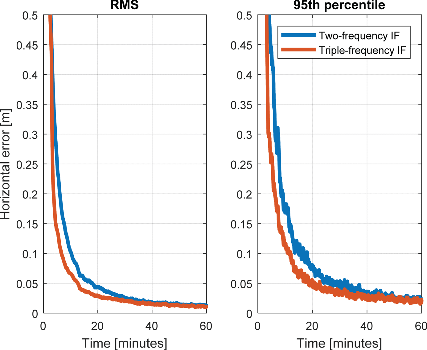
Figure 11. Comparison between the horizontal error achieved using the traditional GPS L1-L5 IF and Galileo E1-E5 IF combinations (blue) and the one obtained by using also the triple-carrier IF combinations that minimise the noise in the narrow-lane ambiguity observable (red).

Table 4. Comparison between the horizontal convergence times obtained from using only the two-frequency IF combinations and also the triple-carrier IF combination that minimise the error in the narrow-lane ambiguity.

RMS and 95th percentile over 50 simulations. Values in units of minutes.

In all cases, after the convergence pattern, the PPP solutions computed from dual- and triple-frequency measurements reach the same precision level.

Unlike the outcomes presented in Deo and El-Mowafy (Reference Deo and El-Mowafy2016), triple-frequency combinations have the potential to improve the convergence time of the float PPP solutions. On the other hand, given the large noise in the triple-carrier IF combinations aimed to enhance the observability of the NL ambiguity observables, they become effective only if they share the same ambiguity value with a more precise IF combination. For this reason, the fractional hardware delays must be corrected for and the EWL and WL ambiguities must be fixed. Therefore, the solution here proposed is not a traditional float PPP solution, but it can be considered float only for the estimation of the NL ambiguity.