2.1. Hydrodynamic parameters for decoupled motions

To derive the equations of motion for an AUV, two coordinate systems, including the earth-fixed coordinate system X_GY_GZ_G and the body-fixed coordinate system X_AY_AZ_A, are defined and shown in Figure 1.

Figure 1. Earth-fixed and body-fixed coordinate systems.

With the assumptions adopted from Fossen (Reference Fossen1994), the AUV equations of motion in the body-fixed coordinate system are obtained as follows:

(1)$$\left\{{\matrix{\dot{u}=\lsqb \lpar Z_{\dot{w}}-m\rpar wq+\lpar m - Y_{\dot{v}}\rpar vr+\lpar X_{u} + X_{u\vert u\vert }\vert u\vert \rpar u+X\rsqb /\lpar m - X_{\dot{u}}\rpar \hfill \cr \dot{v}=\lsqb \lpar X_{\dot{u}}-m \rpar ur+\lpar m-Z_{\dot{w}}\rpar wp+\lpar Y_{v} + Y_{v\vert v\vert }\vert v\vert \rpar v+Y\rsqb /\lpar m - Y_{\dot{v}}\rpar \hfill \cr \dot{w}=\lsqb \lpar Y_{\dot{v}}-m\rpar vp+\lpar m - X_{\dot{u}}\rpar uq+\lpar Z_{w} + Z_{w\vert }\vert \rpar w+Z\rsqb /\lpar m - Z_{\dot{w}}\rpar \hfill \cr \dot{p}=\lsqb \lpar Z_{\dot{w}}-Y_{\dot{v}}\rpar wv+\lpar I_{y}-I_{z}+N_{\dot{r}}-M_{\dot{q}}\rpar rq+\lpar K_{p} + K_{p\vert p\vert }\vert p\vert \rpar p+r_{B_{Z}}mg\cos \theta \sin \phi +K\rsqb /\lpar I_{x} - K_{\dot{p}}\rpar \hfill \cr \dot{q}=\lsqb \lpar X_{\dot{u}}-Z_{\dot{w}} \rpar uw+\lpar I_{z}-I_{x}+K_{\dot{p}}-N_{\dot{r}} \rpar pr+\lpar M_{q} + M_{q\vert q \vert }\vert q \vert \rpar q+r_{B_{Z}}mg\sin \theta +M \rsqb /\lpar I_{y} - M_{\dot{q}} \rpar \hfill \cr \dot{r}=\lsqb \lpar Y_{\dot{v}}-X_{\dot{u}} \rpar vu+\lpar I_{x}-I_{y}+M_{\dot{q}}-K_{\dot{p}} \rpar pq+\lpar N_{r} + N_{r\vert r \vert }\vert r \vert \rpar r+N \rsqb /\lpar I_{z} - N_{\dot{r}}\rpar \hfill}}\right. $$

where X, Y and Z are forces; K, M and N are torques; u, v and w are translational velocities with respect to X_AY_AZ_A; p, q and r are angular velocities with respect to X_AY_AZ_A; x, y and z are positions with respect to X_GY_GZ_G and ϕ, θ and ψ are Euler angles with respect to X_GY_GZ_G. m is the mass and I _x, I _y and I _z are the moments of inertia about X_AY_AZ_A. r _{B Z} is the vertical component of the position vector from the Centre of Gravity (CG) to the Centre of Buoyancy (CB). g is the gravitational acceleration and the remaining 18 parameters ($X_{\dot{u}}$, X _u, X _u|u|, etc.) are the hydrodynamic parameters to be identified through six 1D motions. Table 1 shows the relations between hydrodynamic parameters and decoupled 1D motions.

Table 1. Relations between hydrodynamic parameters and 1D motions.

2.2. Laser image-based AUV position and attitude calculations

The uniqueness of LSHPI is in determining the AUV positions and Euler angles through laser images. The procedures to calculate the AUV positions or Euler angles in each decoupled motion will be presented in the following subsections. Figure 2 shows the assumed geometrical relations between the CG, video camera and laser module of the AUV. All four lengths, including h _camera, h _centre, l _camera and l _laser can be acquired beforehand and are considered as given information.

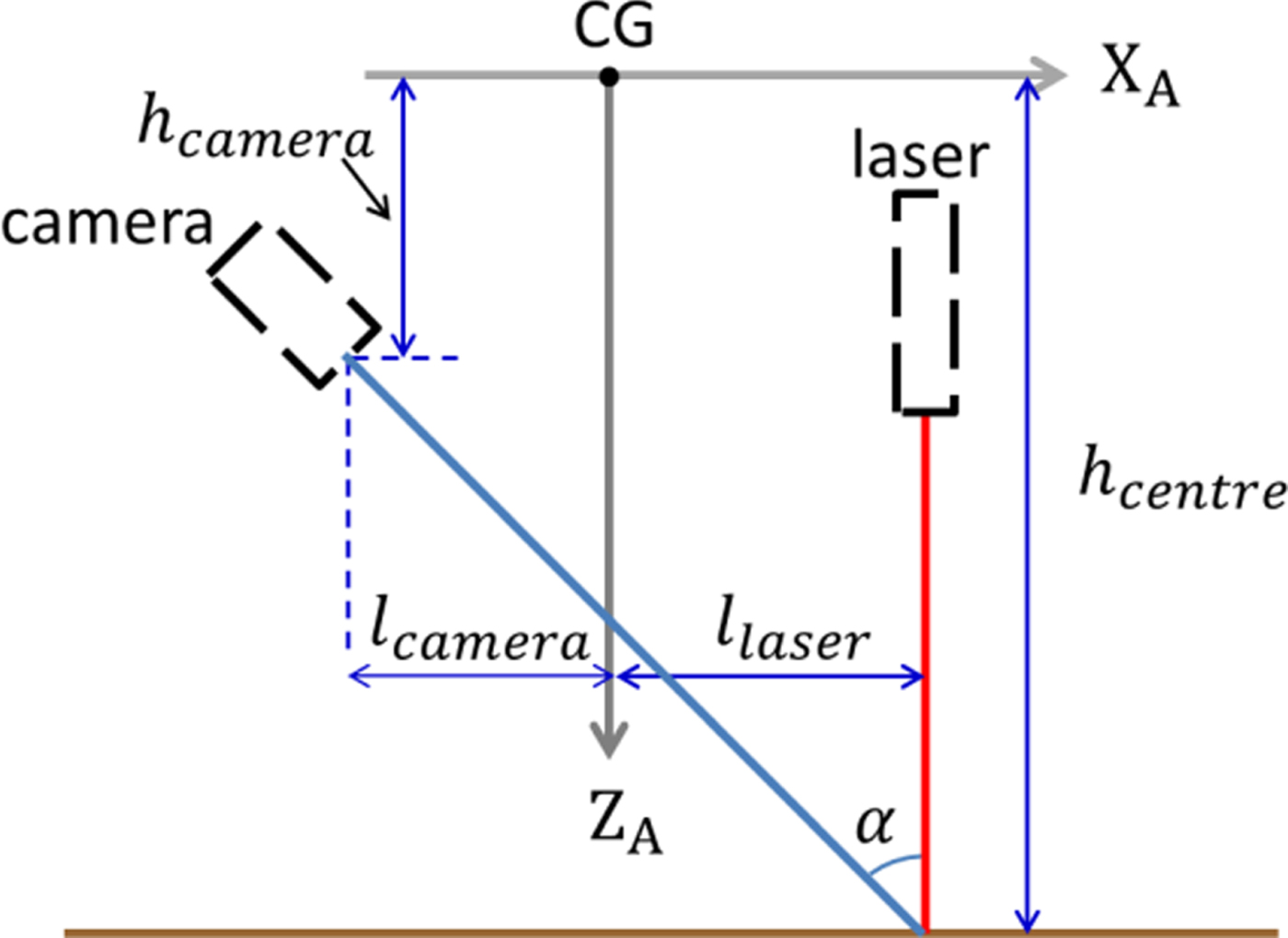
Figure 2. Assumed geometrical relations among the CG, video camera, and laser module of the AUV.

2.2.1. Surge motion

The scanned object for the surge motion has two layers: the upper layer consists of multiple hexagon components; which have the same dimensions and connect one after another. The lower layer is a rectangular board, which is used to locate the scanned object's centre line in a laser image. In general, an AUV cannot initiate a path parallel to the scanned object's centre line, as shown in Figure 3. Thus, before calculating the AUV positions, the angle ψ _S between the AUV moving path and the scanned object's centre line has to be determined through laser images.

Figure 3. Laser image-based AUV position calculation for surge motion.

The procedure to calculate the AUV positions in surge motion is as follows:

1. 1. Obtain the angle ψ _S between the AUV moving path and the scanned object's centre line.

   1. (a) For points A, B, C and D on each of the n laser images, convert their horizontal pixel coordinates to the horizontal coordinates on the laser scanning plane.

   2. (b) Calculate the lengths l _i and r _i, which are the distances from the scanned object's centre line to points $B_{i}^{\prime}$ and $C_{i}^{\prime}$, respectively. The scanned object's centre line is located at the centres between points $A_{i}^{\prime}$ and $D_{i}^{\prime}$, where i = 1, 2,···, n.

   3. (c) Calculate the angles $\psi_{S_{i}}$ using l _i and r _i, where i = 1, 2,···, n. Then find the mean angle ψ _S.

2. 2. Obtain the AUV positions x _i along the moving path.

   1. (a) Calculate $X_{S_{i}}$ using the scanned object's geometrical properties and r _i or l _i, where i = 1, 2,···, n.

   2. (b) Calculate the AUV positions x _i using $X_{S_{i}}$ and ψ _S, where i = 1, 2,···, n.

2.2.2. Sway motion

Although the hexagonal scanned object for surge motion is also applicable to the sway scenario, the simplest scanned object for the sway motion is a rectangular board, as shown in Figure 4. The procedure to calculate the AUV positions during sway motion is as follows:

1. 1. For point A (or B) on each of the n laser images, convert its horizontal pixel coordinate to the horizontal coordinate ξ_i on the laser scanning plane, where i = 1, 2,···, n.

2. 2. Use ξ₁ as the initial point to calculate the AUV positions y _i via Equation (2) as below:

   (2)$$y_{i}=\xi_{i}-\xi_{1} $$
   where $i=1\comma \; \thinspace 2\comma \; \cdots \comma \; n$.

Figure 4. Laser image-based AUV position calculation for sway motion.

2.2.3. Heave motion

A laser line moves vertically in the images as the AUV undergoes a heave motion. As shown in Figure 5, the laser line moves up as the AUV goes down. The procedure to calculate the AUV positions in heave motion is as follows:

1. 1. For each of the n laser images, obtain the laser line's vertical coordinate η_i on the laser scanning plane, where i = 1, 2,···, n.

2. 2. Use η₁ as the initial point to calculate the AUV positions z _i via Equation (3) as below:

   (3)$$z_{i}=\eta_{i}-\eta_{1} $$
   where i = 1, 2,···, n.

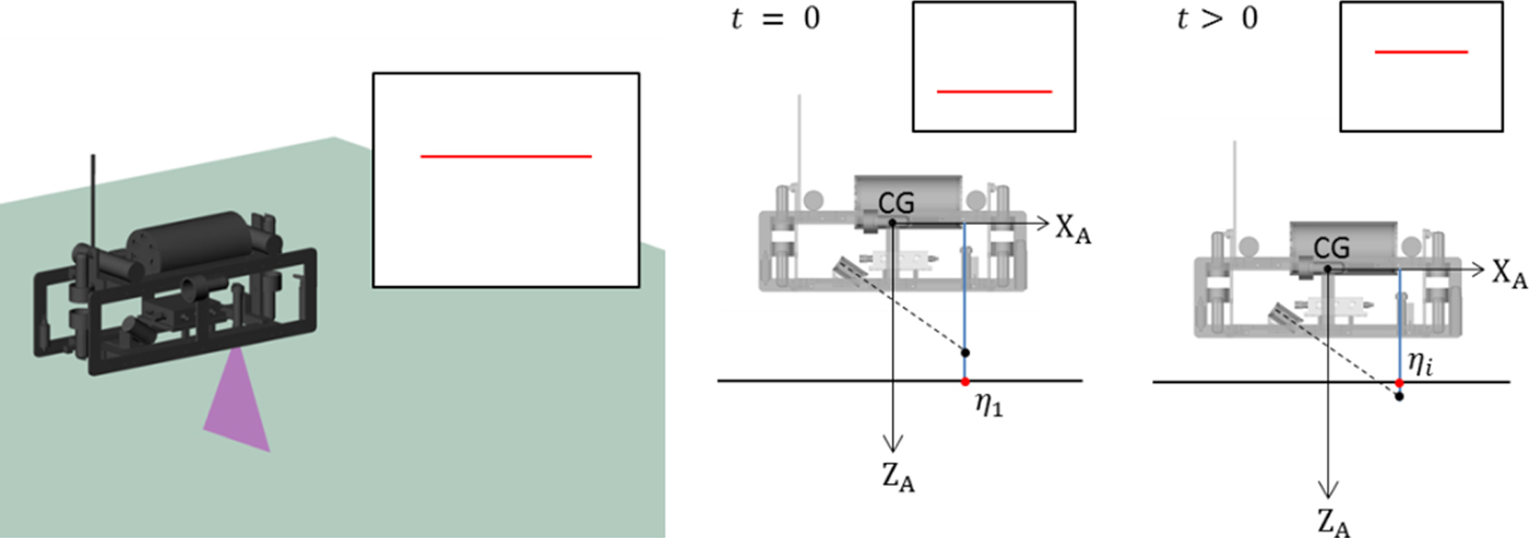
Figure 5. Laser image-based AUV position calculation for heave motion.

2.2.4. Roll motion

A laser line rotates in the images as the AUV undergoes roll motion. As shown in Figure 6, the laser line rotates counterclockwise as the AUV rolls clockwise. The procedure to calculate the AUV Euler angles in roll motion is as follows:

1. 1. For points A and B on each of the n laser images, convert their planar pixel coordinates to the planar coordinates (ξ _i, η _i) on the laser scanning plane, where i = 1, 2,···, n.

2. 2. Calculate the AUV Euler angles ϕ _i using Equation (4) as below:

   (4)$$\tan \phi_{i}=\displaystyle{{\eta_{i_{B}}-\eta_{i_{A}}}\over{\xi_{i_{A}}-\xi _{i_{B}}}} $$
   where i = 1, 2,···, n.

Figure 6. Laser image-based AUV attitude calculation for roll motion.

2.2.5. Pitch motion

A laser line moves vertically in the images as the AUV undergoes a pitching motion. As shown in Figure 7, the laser line moves down as the AUV pitches up. The procedure to calculate the AUV Euler angles in the pitch motion is as follows:

1. 1. For each of the n laser images, obtain the laser line's vertical coordinate η_i on the laser scanning plane, where i = 1, 2,···, n.

2. 2. Calculate the AUV Euler angles θ _i using Equation (5) as below, where η_level is the laser line's position at θ = 0:

   (5)$$\lpar h_{centre}-\eta_{i}\rpar \cos \theta_{i}=l_{laser}\sin \theta _{i}+h_{centre}-\eta_{level} $$

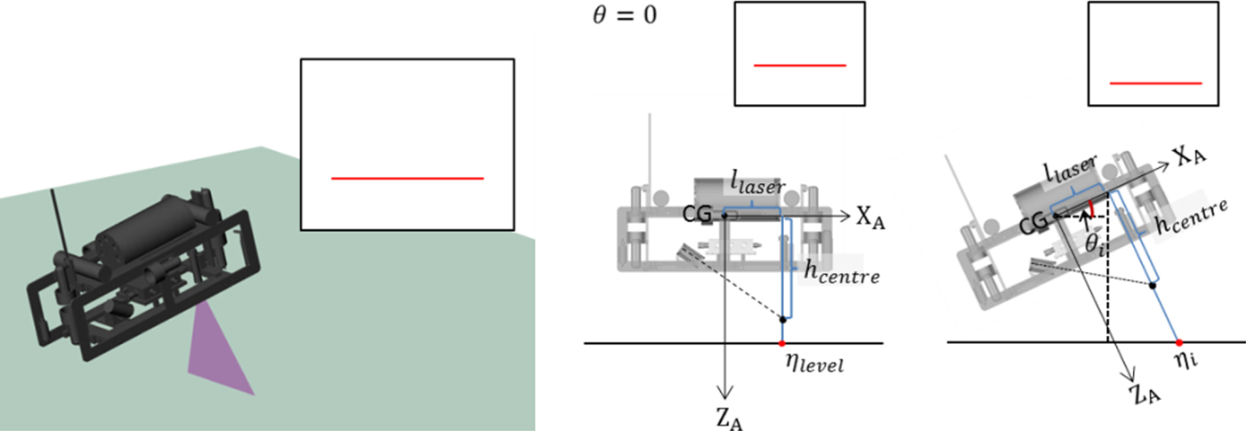
Figure 7. Laser image-based AUV attitude calculation for pitch motion.

2.2.6. Yaw motion

The scanned object for yaw motion is the same as for surge motion, as shown in Figure 8. The procedure to calculate the AUV Euler angles during yaw motion is as follows:

1. (a)–(c) The same as those in step 1 for surge motion.

2. (d) Use $\psi_{S_{1}}$ as the initial angle to calculate the AUV Euler angles ψ _i via Equation (6) as below:

   (6)$$\psi_{i}=\psi_{S_{i}}-\psi_{S_{1}} $$
   where $i=1\comma \; \thinspace 2\comma \; \cdots \comma \; n$.

Figure 8. Laser image-based AUV attitude calculation for yaw motion.

2.3. Evolutionary search for hydrodynamic parameters

Genetic Algorithms (GAs) always operate on a whole population of candidates rather than a single candidate for solution searching. This characteristic improves the chances of a GA reaching the global optimum and also helps GAs avoid being trapped in a local optimum. This characteristic also indicates the inherent parallelism of GAs, which facilitates the distributed implementation of GAs for computational efficiency enhancement (Sivanandam and Deepa, Reference Sivanandam and Deepa2007). A basic GA was implemented in this research to validate the feasibility of the proposed method, LSHPI. Nevertheless, any evolutionary optimisation algorithm can be used in LSHPI. Here, the GA has six objective functions, each of which corresponds to a 1D motion. Thus, for a specific 1D motion, the GA takes the positions or Euler angles obtained through laser images as the input and returns a set of hydrodynamic parameters that minimise the motion's objective function value. As an example, the objective function for surge motion is illustrated below.

The system of equations relating X_A Y_A Z_A to X_G Y_G Z_G for surge motion is as follows:

(7)$$\left\{{\matrix{{\dot{u}}=\lsqb \lpar X_{u} + X_{u\vert u\vert }\vert u\vert \rpar u+X \rsqb /\lpar m - X_{\dot{u}}\rpar \hfill \cr {\dot{x}} = u \hfill}}\right. $$

The position dataset obtained from the laser images is defined as:

(8)$$\hbox{x}_{img}=\lcub x_{img}^{i}\vert i=1\sim n \rcub $$

where $x_{img}^{i}$ is the i-th position value.

The position dataset obtained from Equation (7) with a set of hydrodynamic parameters, $\lcub X_{\dot{u}}\comma \; X_{u}\comma \; X_{u\vert u \vert }\rcub $, is defined as:

(9)$$\hbox{x}_{eof}=\lcub x_{eof}^{i} \vert i=1\sim n \rcub $$

where $x_{eof}^{i}$ is the i-th position value.

Therefore, the objective function for the surge motion is defined as:

(10)$$f\!\lpar X_{\dot{u}}\comma \; X_{u}\comma \; X_{u\vert u \vert } \rpar =\sum_{i=1}^n \vert x_{eof}^{i}-x_{img}^{i} \vert $$

3.1. Laser images created by OpenGL

OpenGL models a spotlight source as restricted to producing a cone of light in a particular direction. In this research, a line-laser is modelled based on the OpenGL spotlight model, such that the line-laser produces a beam of light with a fan angle of 40^° and line thickness of 6 mm. In addition, only the diffuse effect of the laser light is considered in this research. For instance, in Figure 9, the left sub-figure shows an elevation view of the AUV, which performs surge motion and projects a laser light stripe on a hexagon object; the right sub-figure shows a laser image that is seen from the AUV on board camera and consists of several laser line segments, and the discontinuity points on the laser line represent the locations where the object height changes.

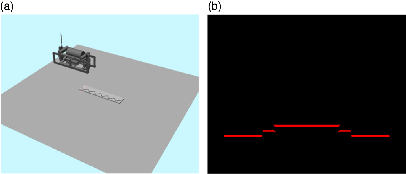
Figure 9. (a) An elevation view of the AUV; (b) a laser image seen from the AUV camera.

3.2. Transformation from image plane coordinates to laser scanning plane coordinates

Figure 10 shows the viewing volume of the camera for creating laser images by OpenGL. A laser image is the current view of the laser scanning plane seen from the camera. In this research, a laser image is specified to have 720 × 576 pixels; in the vertical direction, a laser line has a width of several pixels, and the central pixel is chosen to be the laser line's position.

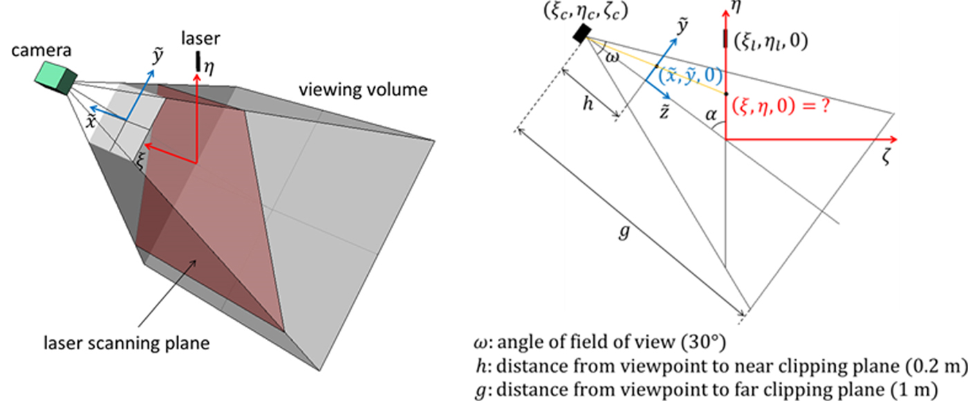
Figure 10. Viewing volume of the camera for creating laser images.

The transformation from the image plane coordinates to the laser scanning plane coordinates is illustrated as follows:

1. 1. Transform the image plane coordinates $\lpar \tilde{i}\comma \; \tilde{j}\rpar $ to the near clipping plane coordinates $\lpar \tilde{x}\comma \; \tilde{y}\rpar $ using ω and h, where ω is the angle of the camera's field of view on the η − ζ plane and h is the distance from the viewpoint to the near clipping plane.

2. 2. Transform the near clipping plane coordinates $\lpar \tilde{x}\comma \; \tilde{y}\rpar $ to the laser scanning plane coordinates (ξ, η) through Equations (11) and (12):

   (11)$$\eta = \eta_{c} + \displaystyle{h\cos \alpha -\tilde{y}\sin \alpha \over h\sin \alpha +\tilde{y}\cos \alpha} \zeta_{c} $$
   (12)$$\xi = \displaystyle{\sqrt{\zeta_{c}^{2}+\lpar \eta_{c}-\eta\rpar^{2}} \over \sqrt{\lpar h\sin \alpha +\tilde{y}\cos \alpha\rpar ^{2}+\lpar h\cos \alpha -\tilde{y} \sin \alpha\rpar^{2}}} \tilde{x}$$
   where (η _c, ζ _c) is the camera's coordinates on the η − ζ plane.

Table 2 lists the lengths and angle denoting the geometrical relations between the CG, video camera and the AUV laser module previously shown in Figure 2. Moreover, Figure 11 shows the dimensions of the scanned object that consists of six hexagonal components on top of a rectangular board and will be used for surge and yaw motions.

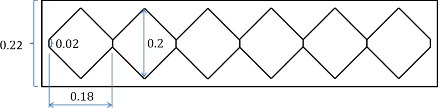
Figure 11. Dimensions (in metres) of the scanned object for the surge and yaw motions.

Table 2. Lengths and angle used in Figure 2.

3.3. Comparison between OpenGL and experimental measurement results

With the proposed LSHPI, the AUV positions and Euler angles are all obtained through laser images. In this research, the feasibility of LSHPI will be validated using the laser images created by OpenGL. Therefore, it is important to compare the measurement errors between the OpenGL measurement results and experimental measurement results. If the OpenGL measurement errors are larger than but close to the real-world measurement errors, the OpenGL measurement results can then be considered to properly include errors from the uncertainty and nonlinearity factors, such as the lens distortion, the roughness of the scanned object, the nonlinearities of the laser beam, etc, as experienced in real-world experiments.

In this research, a test object, with the same shape and dimensions as those in Wang and Cheng (Reference Wang and Cheng2007), is created using OpenGL. Then, the dimension measurements are performed through a laser image seen from the on board camera of a stationary AUV. According to the results, the absolute error for the OpenGL-measured dimensions ranges from 0·08 mm to 1·14 mm, whereas the absolute error for the dimensions obtained through real-world experiments in Wang and Cheng (Reference Wang and Cheng2007) ranges from 0·07 mm to 0·66 mm. The OpenGL absolute error range is larger than the experimental absolute error range, but the two error ranges have the same order of magnitude. Therefore, the OpenGL measurement results can be considered to adequately include errors contributed by the uncertainty and nonlinearity factors associated with the camera, the scanned object and the laser beam, as encountered in the real-world experiments.

3.4. Accuracy for laser image-based AUV position and attitude calculations

In order to investigate the accuracy of the AUV positions and Euler angles obtained by the laser image-based methods illustrated in Section 2, OpenGL animations were implemented and executed. In each OpenGL animation, an AUV performed a 1D motion under the conditions listed in Table 3.

Table 3. Accuracy for laser image-based postion and atttiude calculations in decoupled AUV motions.

For each 1D motion, the calculated positions or Euler angles were compared with actual results to obtain an error range, as shown in Table 3. According to the results, for surge, sway and heave motions, the maximum absolute errors were all less than 1 mm; for roll, pitch and yaw motions, the maximum absolute errors were all less than 1^°.

3.5. Influence of motion disturbances on laser image-based AUV position and attitude calculations

Conducting a specific 1D AUV motion experiment in a water tank usually involves other motion disturbances. Such disturbances will change the laser line locations displayed in laser images, affecting the accuracy of the AUV positions or Euler angles acquired by the proposed laser image-based methods. Therefore, OpenGL animations are implemented and executed, with the moving conditions listed in Table 3 and disturbances listed in Table 4 (or Table 5). Additionally, the term “no effect” in Table 4 and Table 5 means that a specific motion disturbance has no influence on the accuracy for the positions or Euler angles obtained in a particular 1D motion.

Table 4. Influence of motion disturbances on the accuracy for calculated AUV positions.

Table 5. Influence of motion disturbances on the accuracy for calculated AUV Euler angles.

For surge motion, the sway disturbance affects the accuracy of calculated AUV positions if a yaw disturbance exists. Likewise, heave disturbance affects the accuracy of calculated AUV positions if a pitch disturbance exists. Moreover, roll, pitch and yaw disturbances all influence the accuracy of calculated AUV positions. Compared with other errors, the maximum error induced by the pitch disturbance is significant.

For sway motion, the surge disturbance affects the accuracy of calculated AUV positions if the scanned object's centreline is not perpendicular to the sway direction. Compared with other errors, the maximum errors, induced by roll and yaw disturbances, respectively, are both significant.

Figure 12 shows the calculated pitch angles when the AUV pitches up with two different heave disturbances; the calculated AUV pitch angles with a downward heave disturbance are displayed in blue dots, whereas the calculated AUV pitch angles with an upward heave disturbance are displayed in green dots. The absolute errors between the actual and calculated pitch angles at θ = 20^° and θ = −15^° are also shown in Figure 12. Such an absolute error increases significantly when the pitch angle θ becomes negative. This is because, without any motion disturbances, the rate of change of laser line position (η) on the laser scanning plane becomes small when the pitch angle θ turns negative, as shown in Figure 13 As a result, if a heave disturbance exists, when the pitch angle θ becomes negative, the effect of the heave disturbance on the change of laser line position also becomes significant.

Figure 12. Relations between actual and calculated pitch angles with different heave disturbances.

Figure 13. Relations between pitch angle and laser line position on the laser scanning plane without disturbances.

3.6. Hydrodynamic parameter identification for surge motion by LSHPI

This section considers surge motions under three conditions: (1) no motion disturbances exist; (2) a pitch disturbance exists; (3) pitch and yaw disturbances both exist. The influence of the pitch and yaw disturbances on the accuracy of the surge-related hydrodynamic parameters obtained by the LSHPI will be investigated. Table 6 shows the physical properties and the surge-related hydrodynamic parameters of an AUV. The parameters, including $X_{\dot{u}}=-250$, X _u = −20 and X _u|u| = −200, are defined as the actual hydrodynamic parameters in this work.

Table 6. Physical properties and surge-related hydrodynamic parameters of an AUV.

3.6.1. AUV position datasets for OpenGL animations

In this research, position datasets used to move the AUV in OpenGL animations are created by solving the equation of surge motion, with parameters listed in Table 6 and a resultant force X from thrusters, using the fourth-order Runge-Kutta method. Such position datasets are defined as actual position datasets in this work. Figure 14 shows two actual position datasets obtained for X = 4 N and X = 8 N, respectively. For surge animations with pitch disturbances, a total of two position datasets are created by adding the pitch disturbance data, shown in Figure 15(a) and Figure 16(a), to the actual position data for X = 4 N and X = 8 N, respectively. Likewise, for surge animations with both pitch and yaw disturbances, a total of two position datasets are created by adding both pitch and yaw disturbance data, shown in Figure 15 and Figure 16, to the actual position data for X = 4 N and X = 8 N, respectively.

Figure 14. Actual position datasets for a 1-metre surge motion at X = 4 N and X = 8 N.

Figure 15. Artificial pitch and yaw disturbances for surge motion at X = 4 N.

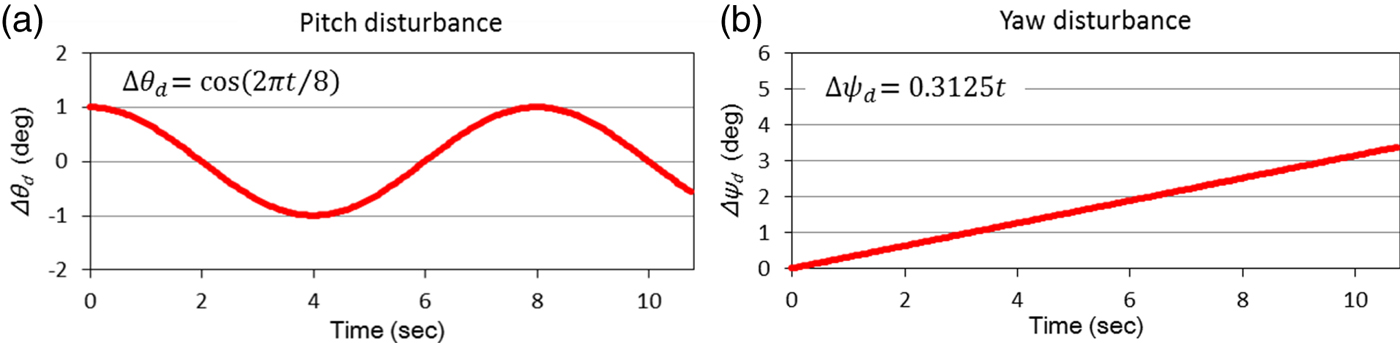
Figure 16. Artificial pitch and yaw disturbances for surge motion at X = 8 N.

3.6.2. AUV positions obtained from laser images

As illustrated in the previous subsection, a total of six OpenGL animations were created for AUV surge motions under three disturbance conditions and two thrust conditions. The laser images taken in each animation are used to obtain the AUV positions for the corresponding surge motion. Additionally, in each animation, the angle ψ _S between the AUV moving path and the scanned object's centreline is set as −4^°.

At each time step, the angle $\psi_{S_{i}}$ between the AUV moving path and the scanned object's centreline can be obtained from each laser image. For example, Figure 17 shows the obtained angles $\psi _{S_{i}}\lpar i =1\comma \; 2\comma \; \ldots\rpar $ at X = 4 N under two different conditions: (1) the AUV moves without disturbances; (2) the AUV moves with both pitch and yaw disturbances. The results illustrate that it is feasible to use the proposed hexagonal scanned object to obtain the angles $\psi_{S_{i}}$ (i = 1, 2, …) and that the deviation from the correct angle value becomes larger when the AUV is passing the common narrow side of two connected hexagon components.

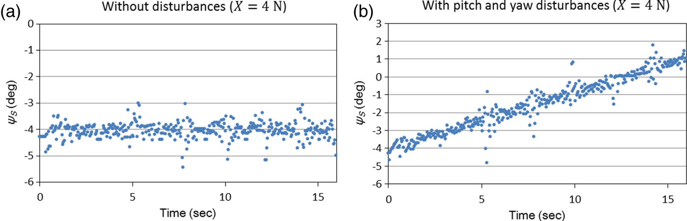
Figure 17. $\psi_{S_{i}}\lpar i =1\comma \; 2\comma \; \ldots$) obtained from laser images.

Figure 18 shows the actual positions and the positions obtained from laser images for the six surge motions with different combinations of thrust and motion disturbance. Table 7 shows the obtained angle ψ _S and the maximum absolute position error in each of the six surge motions. As illustrated earlier in Section 2, the angle ψ _S is the average value of $\psi_{S_{i}} \lpar i=1\comma \; 2\comma \; \ldots$) and is used to calculate the AUV positions in surge motion.

Figure 18. AUV actual positions and positions obtained from laser line images.

Table 7. ψ _S and maximum absolute position error for each of the six surge motions.

3.6.3. GA search for hydrodynamic parameters

The surge-related hydrodynamic parameters are determined through a GA search strategy. The GA takes X = 4 N and X = 8 N position datasets as two inputs and uses the sum of two normalised objective function values as the quality index for each candidate solution, that is, each hydrodynamic parameter set containing $X_{\dot{u}}$, X _u, and X _u|u|. As previously illustrated in Section 2, the smaller the objective function value, the better the solution quality.

Table 8 shows the settings of the GA's parameters. Table 9 shows the search range of each hydrodynamic parameter in the GA. Taking position datasets regarding two thrust conditions as inputs, the GA aims to find a set of hydrodynamic parameters for each of the three disturbance conditions: (1) surge motion without disturbances; (2) surge motion with pitch disturbance and (3) surge motion with both pitch and yaw disturbances. For each of the above conditions, the GA is executed ten times to generate ten optimal hydrodynamic parameter sets among which the best set is selected as the identification result.

Table 8. Settings of the GA's parameters.

Table 9. Search range of each hydrodynamic parameter in the GA.

Table 10 shows the hydrodynamic parameters identified for the three disturbance conditions. When no disturbances exist, the obtained hydrodynamic parameters are very close to the actual parameters. Meanwhile, when a pitch disturbance exists or pitch and yaw disturbances both exist, the obtained hydrodynamic parameters show some differences from the actual parameters.

Table 10. Hydrodynamic parameters identified for three disturbance conditions.

In order to evaluate the effectiveness of the identified hydrodynamic parameters, the positions for a long surge motion, that is, a 5 metre surge motion, are calculated using the three sets of identified hydrodynamic parameters, shown in Table 10, under three different thrusts, X = 4 N, X = 8 N and X = 16N.

The maximum absolute errors between the actual positions and the positions calculated through the identified hydrodynamic parameters are shown in Table 11. The largest absolute error, 80·4 mm, comes from the positions calculated by the hydrodynamic parameters obtained when pitch and yaw disturbances both exist. However, the percentage error for the above absolute error is calculated as 1·61%, which can be considered insignificant. Therefore, the above results indicate that the proposed LSHPI can be used to identify AUV hydrodynamic parameters with sufficient accuracy under moderate motion disturbances.

Table 11. Max. absolute errors between actual and identified-parameter-based positions for 5-m surge motions.