


1. INTRODUCTION
In general, the main approaches to the problem of planning optimal ship trajectories in encounter situations are based on either differential games or on evolutionary programming. The former method has been introduced by Lisowski (Reference Lisowski2005) and it assumes that the process of steering a ship in multi-ship encounter situations can be modelled as a differential game played by all ships involved, each having their strategies. Unfortunately, high computational complexity is its serious drawback. The latter approach is the evolutionary method of finding the trajectory of the own ship, proposed by Smierzchalski and Michalewicz (Reference Smierzchalski and Michalewicz2000). The second approach has recently become especially popular among researchers – it may be applied for finding an optimal path (Zeng, Reference Zeng2003) as well as an optimal collision avoidance manoeuvre (Tsou et al., Reference Tsou, Kao and Su2010). In short, the evolutionary method uses genetic algorithms, which, for a given set of pre-determined input trajectories find a solution that is optimal according to a given fitness function. However, the method's limitation is that it assumes the target's motion parameters do not change and if they do change, the own trajectory has to be recomputed. This limitation becomes serious in restricted waters. If a target's current course collides with a landmass or another target of a higher priority, there is no reason to assume that the target would keep such a disastrous course until the crash occurs. Consequently, planning the own trajectory for the unchanged course of a target will be futile in the majority of such cases. Also, the evolutionary method does not offer a full support to VTS operators, who might face the task of synchronizing trajectories of multiple ships with many of these ships manoeuvring.
Therefore, the author has decided to try a new approach, which combines some of the advantages of both methods: the low computational time, supporting all domain models and handling stationary obstacles (all typical for evolutionary method), with taking into account the changes of motion parameters (changing strategies of the players involved in a game). Instead of finding the optimal own trajectory for the unchanged courses and speeds of targets, an optimal set of safe trajectories of all ships involved is searched for. The method is called evolutionary sets of safe trajectories and one of its earlier versions has been presented in Szlapczynski, (Reference Szlapczynski2009). These earlier versions were either focused on open waters (where the lack of stationary constraints made the task easier) or they simplified the problem of restricted waters by modelling the constraints (landmasses) as polygons. This simplification cannot be applied when we are dealing with the real maps because of their sizes and complexity. Therefore, this time, instead of the simplified polygon modelling, a vector digital map in the open format (MIF) was converted to a raster digital map, which was then used by the computational processes for better performance.
The rest of the paper is organized as follows. In the next section the task – finding sets of safe trajectories – is presented as an optimization problem. Then some basics of the evolutionary approach are given in Section 3, followed by a detailed description of the proposed method in Section 4, which focuses on evolutionary issues specific to the problem. Some simulation results are shown in Section 5 and finally the method's summary and conclusions are given in Section 6.
2. OPTIMISATION PROBLEM
It is assumed that we are given the following data:
• stationary constraints (such as landmasses and other obstacles),
• positions, courses and speeds of all ships involved,
• ship domains,
• times necessary for accepting and executing the proposed manoeuvres.
Ship positions and ship motion parameters are provided by ARPA (Automatic Radar Plotting Aid) and AIS (Automatic Identification System) systems. A ship domain can be determined based on the ship's length, its motion parameters and the type of water region. Since the shape of a domain is dependant on the type of water region, the author has decided to use a ship domain model by Davis (Davis et al., Reference Davis, Dove and Stockel1982), which updated the Goodwin model (Goodwin, Reference Goodwin1975), for open waters and to use a ship domain model by Coldwell (Reference Coldwell1982), which updated the Fuji model (Fuji and Tanaka, Reference Fuji and Tanaka1971), for restricted waters. As for the last parameter – the necessary time – this is computed on the basis of navigational decision time and the ship's manoeuvring abilities. By default a 6-minute value is used here.
Knowing all the abovementioned parameters, the goal is to find a set of trajectories, which minimizes the average way loss spent on manoeuvring, while fulfilling the following conditions:
• none of the stationary constraints are violated,
• none of the ship domains are violated,
• the minimum acceptable course alteration is not less than 15 degrees,
• the maximum acceptable course alteration is not larger than 60 degrees,
• speed alterations are not to be applied unless necessary (collision cannot be avoided by course alteration up to 60 degrees),
• a ship only manoeuvres when she is obliged to,
• manoeuvres to starboard are favoured over manoeuvres to port.
The first two conditions are obvious: all obstacles have to be avoided and, by definition, the ship domain is an area that should not be violated. All the other conditions are either imposed by COLREGS (Cockroft and Lameijer, Reference Cockroft and Lameijer1993) and good marine practice or by economics. In particular, the course alterations less than 15 degrees might be misleading for the ARPA systems (and therefore may lead to collisions) and course alterations larger than 60 degrees are not recommended for efficiency reasons. Also, ships should only manoeuvre when necessary, since each manoeuvre of a ship makes it harder to track its motion parameters for the other ships' ARPA systems.
3. EVOLUTIONARY PROGRAMMING – GENERAL IDEA
Before presenting the details of the method, which solves the optimization problem formulated above, some basic information on evolutionary programming are provided in this section. The general idea of evolutionary programming is shown in Figure 1.

Figure 1. Evolutionary algorithms – general idea.
First, the initial population of individuals (each being a potential solution to the problem) is generated either randomly or by other methods. Usually none of these individuals is optimal or even close to that. Sometimes none of the individuals is acceptable. This initial population is subject to subsequent iterations of the evolutionary algorithm. Each of these iterations consists of the following steps:
1. Reproduction: sets of parents (usually pairs) are selected from all of the individuals and they are crossed to produce offspring. The offspring inherits some features from each parent.
2. Evolutionary operations: the offspring is modified by means of random mutation operators as well as specialized operators dedicated to the problem.
3. Evaluation: each of the individuals (including parents and the offspring) is assigned a value of a fitness function, which reflects the quality of the solution represented by this individual.
4. Succession: the next generation of individuals is selected. The selection is based on the results of the evaluation. Usually the individuals are chosen randomly, with the probability strictly depending on the fitness function value.
The evolutionary algorithm ends when one of the following happens:
• maximum acceptable time or number of iterations is reached,
• satisfactorily high value of fitness function has been reached by one of the individuals,
• further evolution brings no improvement.
The main difference between the evolutionary programming and pure genetic algorithms is that in the former the individuals directly represent the potential solutions to the problem, without being translated to chromosomes first. This allows for specialised operators dedicated to the problem, which, for some classes of optimization tasks, greatly speed up the evolutionary process, resulting in a much smaller number of generations needed and much lower computational time. The method presented in the following section focuses on specialised operators thus fully utilizing the possibilities of evolutionary programming.
4. EVOLUTIONARY SETS OF SAFE SHIP TRAJECTORIES
In this section, the proposed method will be presented in detail, starting with the initial population.
4.1. Generating the initial population
As said in the introduction, each individual (a population member) is a set of trajectories, each trajectory corresponding to one of the ships involved in an encounter. A trajectory is a sequence of nodes, each node containing the following data:
• geographical coordinates x and y,
• the speed between the current and the next node.
The initial population contains three types of individuals:
• a set of original ship trajectories – segments joining the start and destination points,
• sets of safe trajectories determined by other methods,
• randomly modified versions of the first two types – sets of trajectories with additional nodes, or with some nodes moved from their original geographical positions.
The first type of individuals results in an immediate solution in the case of no collisions, or in faster convergence in case of minor constraint violations. The second type provides sets of safe (though usually not optimal) trajectories. Depending on the type of water region, they are mostly generated by the method of planning a trajectory on raster grids (Szlapczynski, Reference Szlapczynski2006a), which enables avoiding collisions with other ships as well as with stationary obstacles (for restricted waters) and by the method of planning a sequence of necessary manoeuvres in open waters (Szlapczynski, Reference Szlapczynski2008).
In the method operating on raster grids, the task of planning a ship trajectory is modelled as finding the optimal route on a raster grid where each cell is either passable (water deep enough to sail safely) or impassable (any kind of still obstacle including the shallows). If the own ship is a “give-way” ship, the cells might also be impassable during the time when “stand-on” targets occupy them.
In the method of planning a sequence of necessary manoeuvres, the targets are split recursively into groups depending on their meeting times with the own ship (early encounters and late encounters) and separate sub-trajectories of the own ship are determined and later merged into one final trajectory.
The third type of individuals (randomly modified individuals of the previous two types) is used to generate the majority of a diverse initial population and thus to ensure a vast searching space.
4.2. Reproduction
In this phase pairs of individuals (parents) are crossed to generate new individuals (offspring). Two types of crossing have been used:
a) An offspring inherits whole trajectories from both parents.
b) Each of the trajectories of the offspring is a crossing of the appropriate trajectories of the parents.
Both types are shown in Figure 2.

Figure 2. Reproduction: (a) inheriting whole trajectories and (b) crossing of trajectories.
4.3. Evolutionary operations – random mutation
Evolutionary operations that have been used include random mutation and three groups of specialized operators. Four types of random mutation operators have been used, all operating on single trajectories. These random operators are:
a) Node insertion: a node is inserted randomly into the trajectory,
b) Node joining: two neighbouring nodes are joined, the new node being the middle point of the segment joining them,
c) Node shift: a randomly selected node is moved (its polar coordinates are altered).
d) Node deletion: a randomly selected node is deleted.
These operators are shown in Figure 3.

Figure 3. Random mutation operators.
A trajectory mutation probability decreases with the increase of the trajectory fitness value, so as to mutate the worst trajectories of each individual first, without spoiling its best trajectories. In the early phase of the evolution all random operators: the node insertion, deletion, joining and shift are equally probable. In the later phase node shift dominates with its course alteration changes and distance changes decreasing with the number of generations. For node insertion and node shift instead of Cartesian coordinates x and y, the polar coordinates (course alteration and distance) are mutated in such a way that the new manoeuvres are between 15 and 60 degrees. As a result, fruitless mutations (the ones leading to invalid trajectories) are avoided for these two operators.
4.4. Evolutionary operations – specialised operators
Specialised operators, responsible for more conscious improving of trajectories (as opposed to random mutation) result in a faster convergence to a solution. The evolutionary operators, which have been used here, can be divided into the following groups, with group 2 only applied for restricted waters.
1) Operators avoiding collisions with prioritised ships. Five types of these operators have been used, all operating on single trajectories. If a collision with a prioritised ship has been registered, an operator is selected depending on the values of the time remaining to a collision and the time remaining to reaching the next node:
a. Segment insertion – if there is only enough time for three course alterations, a new segment is inserted.
b. Node insertion – if there is not enough time for a whole new segment (additional three course alterations), a single node is inserted.
c. First node shift – if there is not enough time for a node insertion (additional two course alterations) and the collision point is much closer to the first node of a segment, the first node is moved away from the collision point.
d. Second node shift – if there is not enough time for a node insertion (additional two course alterations) and the collision point is much closer to the second node of a segment, the second node is moved away from the collision point.
e. Segment shift – if there is not enough time for a node insertion (additional two course alterations) and the collision point is close to the middle of a segment, the whole segment is moved away from the collision point.
None of these operations guarantees avoiding the collision with a given target but they are likely to do so and therefore highly effective statistically, which is enough for evolutionary purposes. These operators are shown in Figure 4.
2) Operators avoiding collisions with stationary obstacles (restricted waters only). If a segment of a trajectory crosses a landmass or other stationary obstacle, similarly as in a case of a collision with a target, depending on the values of the time remaining to collision and the time remaining to reaching the next node, one of the abovementioned five operators is chosen, based on similar rules as in group 1). This is shown in Figure 5.
3) Validations and fixing. This group includes three operators, shown in Figure 6.
a. Node reduction – its purpose is to eliminate all the unnecessary nodes. If a segment, which bypasses a given node by joining its neighbours, is safe, the node is deleted.
b. Smoothing – if a course alteration is larger than 30 degrees, a node is replaced with a segment to smooth the trajectory.
c. Adjusting manoeuvres – each trajectory of an individual is analysed and in the case of unacceptable manoeuvres (such as slight course alterations), the nodes being responsible are moved so as to round a manoeuvre up or down to an acceptable value.

Figure 4. Specialised operators: avoiding collisions with targets.

Figure 5. Specialised operators: avoiding collisions with stationary obstacles.

Figure 6. Validations and fixing operators: (a) node reduction, (b) trajectory smoothing and (c) trajectory adjusting.
4.5. The evaluation of an individual
The basic piece of data used during the evaluation phase of the evolutionary process is the average way loss computed for each individual (a set of safe trajectories). Some of the constraints must also be taken into account during the evaluation. These include violations of ship domains and violations of stationary constraints (restricted waters): they must be penalized and those penalties must be reflected in the fitness function. However, as for the other constraints, representing them in the fitness function would result in a very slow progress of the evolutionary algorithm. Therefore some of the constraints are applied as validating and fixing functions (already described in Section 4.4)
Violations of ship domains and stationary constraints are penalized as follows. For each ship and its set of stationary constraint violations, an obstacle collision factor is computed as given by Equation (4). For each ship and its set of prioritised targets a ship collision factor is computed as given by Equation (3). The reason why only collisions with prioritised targets are represented in evaluation is because the manoeuvres must be compliant with COLREGS. If a ship is supposed to stay on its course according to the rules, the collision is ignored so as not to encourage a manoeuvre.
In case of an encounter with a prioritised target, the author's measure – approach factor f min (Szlapczynski, Reference Szlapczynski2006b) is used to assess the risk of collision. It is defined as follows:
1. First, for given vectors of positions of an own ship and a target ship, the momentary approach factor of the own ship f(t) is defined: f(t) is equal to the scale factor of the largest domain shaped area that is free from target ships. (In other words – after multiplying each of the domain's dimensions by the momentary approach factor, the closest target ship will be placed on the boundary of the thus enlarged, or shrunk, domain).
2. Then the approach factor for a given situation of approach to the target ship f min is defined: f min is equal to the minimal value that is reached by the momentary approach factor of the own ship during the time when the distance between two ships is less than some given threshold distance. (In other words: approach factor is the largest domain-shaped area that is predicted to remain free of other ships throughout the whole encounter situation).
Based on the approach factor values and other parameters, each individual (a set of trajectories) is assigned a value of the following fitness function (1):
sf i – ship collision factor of the i-th ship computed over all prioritised targets:
of i – obstacle collision factor of the i-th ship computed over all stationary constraints:
- n
– the number of ships [/],
- m
– the number of stationary constraints [/],
- i
– the index of the current ship [/],
- j
– the index of a target ship [/],
- k
– the index of a stationary constraint [/],
- fmin i,j
– the approach factor value for an encounter of ships i and j [/],
- trajectory_length i
–the total length of the i-th ship's trajectory [nautical miles]
- trajectory_cross_length i
– the total length of the parts of the i-th ship's trajectory which violate stationary constraints [nautical miles]
The only differences between open waters and restricted waters here are different domain models used and obstacle collision factor of i being equal to 0 for open waters. To detect the stationary constraint violations of an individual, all of its trajectories are checked, segment-by-segment. Analogically, to detect domain violations of an individual, all of its trajectories are checked against each other to find potential collision points.
4.6. Succession
A number of selection methods have been tried by the author with the most successful being the truncation method (with the truncation threshold of 50%). In this method the random factor is eliminated and the highest-ranked individuals constitute the next generation. Although this kind of selection means a loss of diversity (and thus the risk of stopping at local optimums), it has the benefit of a fast convergence to a solution. When combined with specialised operators described in Section 4.4, the solution, which the process converges to, is usually close to the optimal one.
5. EXAMPLE SIMULATION RESULTS
The correctness of the method has been verified by the author through a series of simulation experiments involving up to 12 potentially colliding ships. Usually, an acceptable set of trajectories would be found for the initial population of 50 individuals in 30–50 generations with further generations bringing only minor progress and the near optimal solution would be found before completing 100 generations. The computational time on a standard PC machine, for a typical scenario, varied from 10 to 30 seconds depending on the number of ships and the domain models used. Some example simulation results, generated by the method, are presented, covering encounter situations in open and restricted waters. In all the presented cases, the speeds of all ships are equal and their initial courses are such that the ships would collide with either a landmass or each other. The horizontal and vertical distances on pictures are not equal due to map projection (simple latitude/longitude projection). Landmasses are surrounded with dotted areas, which the ships should not violate (additional stationary constraints).
In Figure 7 an encounter of three ships in open water is shown. The final set of trajectories looks as follows: Ship 2 gives way to Ship 1 and Ship 3 gives way to both Ship 1 and Ship 2. Both collision avoidance manoeuvres are to starboard.

Figure 7. A crossing encounter of three ships in open waters.
In Figure 8 a crossing encounter of two ships is shown. Ship 2 manoeuvres to port to pass safely an island. Ship 1 manoeuvres to starboard to avoid collisions with an island and to pass astern of Ship 2.

Figure 8. A crossing encounter of two ships in restricted waters.
In Figure 9 a head-on encounter of two ships in restricted water is shown. Both ships manoeuvre to their starboard to avoid collisions with each other, while keeping a safe distance from the landmass throughout the passage.

Figure 9. A head-on encounter of two ships in restricted waters.
In Figure 10 an encounter of three ships in restricted water is shown. Ship 1 changes its course to avoid collision with an island. Ship 2 gives way to Ship 1 by altering its course to starboard. Ship 3 manoeuvres to starboard to avoid collisions with both Ship 1 and the landmass.
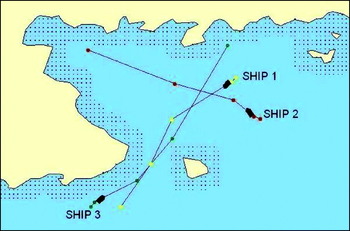
Figure 10. An encounter of three ships in restricted waters.
In Figure 11 an encounter of four ships in restricted water is shown. All ships manoeuvre to avoid collisions with each other and the islands. Ship 1 and Ship 2 manoeuvre to their starboards to avoid collisions with the islands, while leaving enough room for Ship 3 and Ship 4 to pass safely. Ship 3 and Ship 4 manoeuvre to their port to avoid collisions with the islands while keeping right from Ship 1 and Ship 2. Additionally Ship 1 and Ship 3 give way to ships on their starboards – Ship 2 and Ship 4 respectively.

Figure 11. An encounter of four ships in restricted waters.
6. SUMMARY AND CONCLUSIONS
In the paper a new method of solving encounter situations – evolutionary sets of safe trajectories – has been presented. The method is a generalization of evolutionary trajectory determining. A set of trajectories of all ships involved, instead of just the own trajectory, is determined. The method avoids violating ship domains and stationary constraints, while obeying the COLREGS and minimizing total way loss computed over all trajectories. Because of its low computational time the method can be applied to onboard collision-avoidance systems and VTS systems. In the former, in the case of simple scenarios (where ship priorities are clearly described by COLREGS), the method is able to predict the most probable manoeuvre of a target and plan own ship manoeuvre in advance, so that own manoeuvre could be initiated as soon as the target's manoeuvre is executed. In the latter, due to central planning, it could successfully solve any given scenario involving multiple ships and stationary constraints. Further research on the method is planned and it will focus on VTS-specific issues and on planning ship trajectories on Traffic Separation Schemes with high ship density.
ACKNOWLEDGMENTS
The author thanks the Polish Ministry of Science and Higher Education for funding this research under grant no. N N516 186737.


