1. INTRODUCTION
The troposphere is the lowest part of the Earth's atmosphere extending to a height of approximately 15 km, composed of dry gases and water vapour. The troposphere causes errors in GPS measurements both through signal path bending and the alteration of the electromagnetic wave velocity. The troposphere as a non-dispersive medium at the GPS frequencies does not have a frequency dependent delay such as ionospheric layers have, and the actual delay cannot be measured using dual frequency transmission. For high-accuracy positioning and also for meteorological applications, accurate estimation of the atmospheric path delay of GPS signals is necessary. The magnitude of the tropospheric delay depends on the refractive index of the atmosphere along the propagation path. Without proper compensation, tropospheric delay can cause pseudo-range and carrier-phase errors from about 2 m for a satellite in the zenith direction to more than 20 m for a low-elevation satellite, below 10° elevation (Ueno et al. Reference Ueno, Hoshinoo, Matsunaga, Kawai, Nakao, Langley and Bisnath2001).
The refractivity of the troposphere can be divided into hydrostatic and wet components. The refractive index can be expressed as the sum of the hydrostatic or ‘dry’ and non-hydrostatic or ‘wet’ refractivities. These two components have different effects on the propagation of the GPS signal. The hydrostatic component contributes to approximately 90% of the total tropospheric delay. It can be modelled pretty accurately with an error of less than 0·5 m using standard atmospheric models for dry delay based on the laws of ideal gases, assuming layers of constant refractivity with no temporal variation. This error can be considerably reduced if temperature and surface pressure measurements are available. The wet component is much more difficult to model efficiently, as the variation of water vapour in the atmosphere varies greatly with time and location. Most of the water vapour in the atmosphere occurs at heights below 4 km, which particularly affects signals from low elevation satellites that have a longer propagation path length through the troposphere. Fortunately, the wet delay contributes only 10% to the total tropospheric delay.
2. TROPOSPHERIC DELAY MODELS
To estimate the combined zenith delay due to wet and dry components, a model of the standard atmosphere is usually used. Models that do not require real-time meteorological input use average and seasonal variation data related to the receiver's latitude and day-of-year. WAAS/EGNOS is such a “navigation-type” model that provides an estimate of the zenith tropospheric delay, which is dependent on empirical estimates of five meteorological parameters – pressure, temperature, water vapour pressure, temperature lapse rate and water vapour lapse rate. Values of these five meteorological parameters are computed from the values given in a table of meteorological parameters for tropospheric delay, relevant to the receiver height, latitude and day of the year (Penna et al. Reference Penna2001, Ueno et al. Reference Ueno, Hoshinoo, Matsunaga, Kawai, Nakao, Langley and Bisnath2001). Values in the table are estimates of the yearly averages of the parameters and their seasonal variations, derived mainly from North American meteorological data.
Real-time surface meteorological parameters are necessary to avoid failure of a tropospheric delay model under conditions when storm fronts pass, causing large gradients in temperature, pressure and humidity (Markezic et al. Reference Markezic, Filjar and Juricic2000). That is the reason for improving tropospheric delay estimation by employing various surface meteorological parameters in the appropriate tropospheric delay models. A tropospheric correction mapping function is used to determine the delay for different satellite elevation angles (>5°). Two of the best performing prediction models are Saastamoinen and Hopfield.
In the Hopfield model, the total tropospheric delay is expressed as the sum of the dry and wet components:
where p is the atmospheric pressure in hPa, T is the temperature in Kelvin, E is the elevation angle in degrees and e is the partial pressure of water vapour in hPa (Ueno et al. Reference Ueno, Hoshinoo, Matsunaga, Kawai, Nakao, Langley and Bisnath2001).
Tropospheric delay using the Saastamoinen model comprising both dry and wet components is computed as:

where Φ is the latitude of the receiver in radians, h is the orthometric height of the receiver in km, p is the atmospheric pressure in hPa, e is the partial pressure of water vapor in hPa, T is the temperature in Kelvin (Cove et al. Reference Cove, Santos, Wells and Bisnath2004).
Research work presented in many references has examined the performance of many currently available tropospheric delay models used in geodesy and indicated that the zenith delay model of Saastamoinen is generally superior to all others (Cove Reference Cove, Santos, Wells and Bisnath2004, Reference Cove2005, Farah et al. Reference Farah, Moore and Hill2005, Haase et al. Reference Haase, Ge, Vedel and Calais2002, Mendes et al. Reference Mendes, Collins and Langley1995, Musa et al. Reference Musa, Wang, Rizos, Lee and Mohamed2004, Penna et al. Reference Penna2001, Ueno et al. Reference Ueno, Hoshinoo, Matsunaga, Kawai, Nakao, Langley and Bisnath2001).
As we have no International GPS Service (IGS) station in Croatia, there is no available measured tropospheric delay data for our region. To verify the accuracy of tropospheric delay models, we therefore used data obtained from two dislocated IGS stations, one located in Zimmerwald (Switzerland) and the other in Victoria (Canada), both at middle latitudes similar to Croatia. Meteorological data were also available for these stations. A comparison of the measured zenith path delay (ZPD) values and the values computed using the Saastamoinen and Hopfield models using meteorological data for the same locations was performed. To check how efficiently the Saastamoinen and Hopfield models respond to different surface meteorological parameters, we selected for each station two six-day intervals comprising both stable as well as unstable weather conditions with large gradients in temperature and pressure.
Figure 1 presents the measured zenith path delay at IGS station Zimmerwald, Switzerland and the computed values of the tropospheric delay using the Saastamoinen and Hopfield models with available meteorological data. Figure 2 represents the values of the tropospheric delay for Victoria, Canada.

Figure 1. Values of the tropospheric delay at Zimmerwald, Switzerland during stable and unstable weather conditions within two six-day periods.

Figure 2. Values of the tropospheric delay at Victoria, Canada during stable and unstable weather conditions within two six-day periods.
These figures show good agreement between the measured zenith path delay and the tropospheric delay obtained using meteorological surface measurements with the Saastamoinen and Hopfield models.
From Figures 3 to 6 we can analyse the calculated residuals and mean values of the tropospheric delay between ZPD and the Hopfield and Saastamoinen models for both locations. The Saastamoinen model shows slightly better performance with a lower mean value than the Hopfield model. The largest difference of the tropospheric delay values for both locations is less then 45 mm, and the mean value varies between 8 and 20 mm.

Figure 3. Residual and mean value of the tropospheric delay for ZPD/Hopfield model at Zimmerwald, Switzerland.

Figure 4. Residual and mean value of the tropospheric delay for ZPD/Saastamoinen model at Zimmerwald, Switzerland.

Figure 5. Residual and mean value of the tropospheric delay for ZPD/Hopfield model at Victoria, Canada.

Figure 6. Residual and mean value of the tropospheric delay for ZPD/Saastamoinen model at Victoria, Canada.
3. EVALUATION OF TROPOSPHERIC MODELS
After successfully proving the accuracy of the Saastamoinen and Hopfield models, our decision was to use the Saastamoinen model as a reference in our study and compare it to the WAAS/EGNOS “navigation-type” model, that does not require real-time meteorological input (Penna, Reference Penna2001, Farah et al, Reference Farah, Moore and Hill2005). The purpose of our study was to check how the computed values of the tropospheric delay of the EGNOS model correspond to the values estimated using the Saastamoinen model and the measured meteorological parameters for particular locations in Croatia. The geographical environment of these locations is shown in Figure 7. Our study utilised meteorological data for the 12-month period from two locations in Croatia, chosen to allow estimation and comparison of the tropospheric delay in all seasons in the continental part of the country (Zagreb) and in the coastal environment (Zadar). Averaged daily values of meteorological data for the year 2006 were obtained from the Meteorological and Hydrological Institute of Croatia. The computed values of five meteorological parameters for the EGNOS model interpolated for Zagreb and Zadar latitudes are presented in Table 1.

Figure 7. Selected locations in the continental and coastal part of Croatia. (The map is produced by the U.S. Central Intelligence Agency.)
Table 1. Computed average values of parameters for EGNOS model.

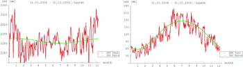
These two locations were selected to allow comparison of two different climatic areas, Zagreb with continental and Zadar with Mediterranean climate. Figure 8 shows the total zenith tropospheric path delay values comparing the EGNOS empirical model and the values obtained using the Saastamoinen model, computed over the one-year period for Zadar and Zagreb. These curves show fairly good agreement with seasonal variations of tropospheric delay on both locations. Examining the curves in Figure 8, we can notice that the EGNOS model has a minimum of the tropospheric delay at the end of January and the Saastamoinen model has a minimum at the beginning of March on both locations. This shift of the minimum of the curves is caused by unusual atmospheric conditions in February and March in the year 2006 with the deviation from normal average meteorological data used in EGNOS model. There were much higher temperatures and lower pressure values than average in the beginning of March that caused the shift of the tropospheric delay minimum.

Figure 8. Zenith total tropospheric delays from 01 January to 31 December 2006 in Zadar (left) and Zagreb (right).
The residuals presented in Figure 9 shows that the maximum tropospheric delay difference between the EGNOS model and the Saastamoinen model is 95 mm for Zadar and 75 mm for Zagreb. The mean values range from 22 mm for Zagreb to 27 mm for Zadar, which is unexpectedly good. The residual curves show two peaks of the residual tropospheric delay components for 30 May and 1 November on both locations, with much lower computed values of the tropospheric delay for the Saastamoinen model than for the EGNOS model shown in Figure 8. Analysing meteorological data for these intervals we noticed that these peaks were probably caused by an extremely rapid drop of the air pressure on these days.

Figure 9. Residual tropospheric delay component over the one-year period for Zadar (left) and Zagreb (right).
To make a better analysis of the tropospheric delay behaviour, our next step was to separate dry and wet components of the tropospheric delay. This should allow more detailed analysis of the compliance of the EGNOS and Saastamoinen tropospheric models within the one-year period and distinguish between different influences. Figures 10 and 11 show the tropospheric ZPD delay for separated wet and dry components for Zadar and Zagreb for EGNOS and Saastamoinen models.

Figure 10. Separated dry (left) and wet (right) components of ZPD for Zadar.

Figure 11. Separated dry (left) and wet (right) components of ZPD for Zagreb.
Analyses of the curves of wet and dry components show very good agreement between EGNOS and Saastamoinen models. The wet component curves apparently show better compliance than the dry components, but this is not the case. Figures 12 and 13 represent residuals and mean values of the delay for Zadar and Zagreb respectively.

Figure 12. Residuals and mean values of dry (left) and wet (right) components for Zadar.

Figure 13. Residuals and mean values of dry (left) and wet (right) components for Zagreb.
The maximum difference between the dry components of the EGNOS and Saastamoinen models for Zadar and Zagreb is less than 50 mm, and for the wet component, less than 90 mm for Zadar and 80 mm for Zagreb. The mean value of the difference for the dry component at both locations is 12 mm, and for the wet component 20 mm in Zagreb and 26 mm in Zadar. This clearly shows that the dry component was modelled better than the wet component, as the compliance is better.
4. CONCLUSIONS
Evaluation of the total tropospheric zenith delays obtained with the EGNOS model and using the Saastamoinen model has allowed assessment of the quality of the EGNOS model. The residual tropospheric delay on both locations showed no significant variations over the year. Separating dry and wet components of the tropospheric delay indicated very good correlation between these models, even for the wet component which is usually much more difficult to model efficiently. The maximum zenith delay difference between these models was in the range of 1 cm to 10 cm, which agrees well with other studies (Penna, Reference Penna2001, Farah et al., Reference Farah, Moore and Hill2005). Although the EGNOS model cannot accommodate changes in the tropospheric delay caused by fast weather changes, it showed remarkably good agreement with the Saastamoinen model. The EGNOS model is computationally simple and gives good accuracy in simulating the mean tropospheric delay. Adding real time surface meteorological data we can achieve very good estimation of the tropospheric delay with sub-seasonal variations, but with much more complexity. For the future, our intention is to analyse the tropospheric delay for other locations in Croatia comprising different latitudes, and also to include meteorological data for several years.
ACKNOWLEDGEMENT
The work described in this paper was conducted under the research project: “Environment for Satellite Positioning” (036-0361630-1634), supported by the Ministry of Science, Education and Sport of the Republic of Croatia.