1. INTRODUCTION
Although navigation technology has considerably improved, incidents of collisions between ships still occur. Finding a collision-free path is the main task in collision avoidance problems. Marine accident surveys have shown that more than 80% of collision accidents are caused by the negligence and irresponsibility of navigators (Zhang et al., Reference Zhang, Yan, Yang and Wall2013; Sormunen et al., Reference Sormunen, Hanninen and Kujala2016). Therefore, intelligent collision avoidance technology has become one of the key technologies for achieving ship automation in recent years.
Although considerable investments in intelligent collision avoidance have been made, there are still many shortcomings in collision avoidance decisions involving multiple ships. Most current collision avoidance studies have assumed that one ship is implementing collision avoidance strategies while other target ships maintain their headings. To learn the intentions of other ships, communication between ships becomes important. Kim et al. applied distributed algorithms in collision avoidance research and proposed some improvements over traditional methods. For example, in the distributed local search algorithm (DLSA) (Kim et al., Reference Kim, Hirayama and Park2014) ships exchange intentions with each other. The distributed tabu search algorithm (Kim et al., Reference Kim, Hirayama and Okimoto2015) introduced a tabu search technique to avoid local optima. The distributed stochastic search algorithm (Kim et al., Reference Kim, Hirayama and Okimoto2017) changes ship intentions in a random manner to reduce the number of communications between ships. In this paper, a distributed algorithm principle is applied, and information for the entire route is used in communication between ships. We suggest a new improvement function that considers the safety and economy of the entire trajectory as a standard for avoidance in scenarios with multiple ships. This approach can not only reduce the collision avoidance operations of ships but also reduce the number of communications between ships in the whole collision avoidance planning.
Communication between ships can effectively simplify the complexity of multi-ship encounters, but detection of danger of collision between ships remains difficult. Szlapczynski and Szlapczynska (Reference Szlapczynski and Szlapczynska2016) proposed using the ship domain for risk calculations considering the shortcomings of closest point of approach (CPA) calculations. The ‘collision diameter’ used by Altan (Reference Altan2019) considers the probability of maritime accident. Kozynchenko and Kozynchenko (Reference Kozynchenko and Kozynchenko2018) applied fuzzy theory and neural networks to predict collision risks. These methods may struggle to make accurate judgements if the trajectory of a ship is nonlinear, however, so it is necessary to adopt a more effective method to assess risk. Huang et al. (Reference Huang, van Gelder and Wen2018) used the velocity obstacle algorithm to monitor the risk of ship collisions. Shi et al. (Reference Shi, Junda, Tengli, Chuan and Jian2018) applied the velocity obstacle algorithm to solve a multi-agent collision avoidance problem. The above studies found that the velocity obstacle algorithm can assess the collision risk of a ship and rapidly find a collision-free solution in multiple-obstacle scenes. Therefore, in this paper, combined with the distributed algorithm principle, the velocity obstacle algorithm is used to solve the collision risk assessment problem in multi-ship scenarios when the trajectory intention of the target ship is known.
There are currently many methods to plan a collision avoidance path. For example, Lisowski (Reference Lisowski2018) applied differential games for collision avoidance planning. Additionally, evolutionary computation methods have been used to find the optimal path (Szlapczynski and Szlapczynska, Reference Szlapczynski and Szlapczynska2012), and genetic, artificial potential fields and particle swarm optimisation algorithms have been applied to find the optimal path in automatic collision avoidance (Kang et al., Reference Kang, Chen, Zhu and Wang2018; Ni et al., Reference Ni, Liu, Cai and Wang2018; Lyu and Yin, Reference Lyu and Yin2019). In this paper, considering the need to plan entire collision avoidance paths at a given time and meet the relevant safety and economic objectives, a multi-objective algorithm is used to select the collision avoidance path. In the case of multiple ships, however, the Pareto front may be discontinuous. Therefore, it is difficult to find all Pareto-optimal solutions using the algorithm based on a non-Pareto criterion, and an algorithm based on the Pareto criterion will have very slow convergence. The bi-criterion evolution (BCE) algorithm can effectively solve these problems (Li et al., Reference Li, Yang and Liu2016), because the entire trajectory can be represented by four variables, namely: the time and range of action at a given avoidance point and the time and range of action at a given resumption point. These four variables are taken as the parameters of the algorithm optimisation to find the desired avoidance path.
In summary, in this paper, we use a distributed algorithm to communicate the intentions of avoidance among ships. Under the condition of knowing the trajectory of the target ship, the velocity obstacle algorithm is used to assess the corresponding danger. Additionally, based on the velocity obstacle method, we propose a new method to calculate the degree of risk, which is regarded as a goal of path optimisation. Because the essence of the velocity obstacle method is related to the ship domain, and the shape of the ship domain is irregular, we apply ship domains related to the ship itself for all ships here instead of expanding the ship domain of the target ship. BCE is used to select the trajectory of the ship, and a population updating method based on the ant lion algorithm is introduced to replace and improve upon the crossover operator in BCE. We suggest a new improvement function considering safety and efficiency to discriminate the action ship in each communication. Therefore, the method adopted in this paper reduces the number of communications in the process of distributed algorithm, and the velocity obstacle method in the field of aggregate ships can better judge the danger between ships. In addition, a new dangerous calculation method is proposed to make it more suitable for a multi-ship collision avoidance environment. By using the multi-objective algorithm instead of deterministic action time as the distributed algorithm, the collision avoidance trajectory has greater autonomy.
The rest of the paper is organised as follows. Section 2 mainly explains the principles of the velocity obstacle algorithm and the distributed algorithm and the calculation of the parameters required for collision avoidance. The principle of the BCE algorithm embedded in the ant lion algorithm and the specific application of the method in ship collision avoidance are explained in Section 3. In Section 4, the simulation examples based on this method are given for multi-ship encounters. Finally, a summary and conclusions are given in Section 5.
2. DESCRIPTION OF THE COLLISION AVOIDANCE METHOD
2.1. Danger model based on velocity obstacle algorithm
The velocity obstacle (VO) algorithm has been applied in many fields, such as vehicles, robots, and unmanned aerial vehicles, to avoid collisions (Mercado et al., Reference Mercado Velasco, Borst, Ellerbroek, Van Paassen and Mulder2015; Wang, Reference Wang2015; Lee et al., Reference Lee, Jeon and Oh2017). Because the VO algorithm itself provides not only conflict detection results but also an optional speed set, this method has gradually been applied in the ship field in recent years (Huang et al., Reference Huang, van Gelder and Wen2018; Song et al., Reference Song, Su, Dong and Shen2018). In the velocity space, the collision risk can be converted into visible velocity contours. Figure 1 shows the principle of the VO algorithm. The speed of the ‘own ship’ (OS) is  $\vec{v}_{o} $, its position is P o (t), and the speed of the target ship (TS) is
  $\vec{v}_{t}$, and its position is P t (t). Therefore, at time t, the collision between OS and TS is defined as follows:
 $$P_o (t)\in P_t (t)\oplus ConfP(O,R)$$
where ConfP is an abbreviation of ‘conflict position’, which depends on the shape and size of the ship. The operation ⊕ is the Minkowski addition. Therefore, for a course change of TS in the collision process, OS is informed, and the VO set can be expressed as follows:
 $${\rm VO} = \bigcup\limits_{t_f}^\infty {\left( {\displaystyle{{P_j{\rm (}t_f{\rm )}-P_j{\rm (}t_0{\rm )}} \over {t_f-t_0}}\oplus \displaystyle{{ConfP(O,R)} \over {t_f-t_0}}} \right)} $$
 where t f is the time when two ships collide and t 0 is the initial time. As shown in Figure 1, a VO is a cone in the velocity space. To determine whether there is a risk of collision between two ships, it is necessary only to determine whether the velocity vector  $\vec{v}_{o} $ of OS is in the above VO set.

Figure 1. Graphical interpretation of the VO set: (a) scenario in geographical space; (b) VO set composed of the relative velocities; the ship domain is treated as ConfP; (c) transformation of the VO set through  $\vec{v}_{t}$.
In this paper, the VO algorithm performs well because the communication between ships can determine the behaviour of each ship. According to Szlapczynski and Szlapczynska (Reference Szlapczynski and Szlapczynska2016), there are certain defects in CPA discrimination. Thus, ConfP is represented as the ship domain here, and the quaternion ship domain is adopted (Wang, Reference Wang2013), as shown in Figure 1. Because the ship domain is irregular, it is unreasonable to consider only a certain proportion of the TS to be enlarged. Therefore, the ship domain of each ship should be retained in the form of a dual ship domain. In this way, there are two collision risk values for the two ships. If one value is beyond the collision limit, it is considered that a collision will occur. The specific formula for the ship domain is as follows (Wang, Reference Wang2013):
 $$\begin{cases} R_{{\rm fore}} =\left( {1+1{\cdot}34\sqrt {A_D^2 +( {{D_T } / 2} )^2} } \right)L \\ R_{{\rm aft}} =\left( {1+0{\cdot}67\sqrt {A_D^2 +( {{D_T } / 2} )^2} } \right)L \\ R_{{\rm starb}} =( {0{\cdot}2+{D_T } / L} ) L \\ R_{{\rm port}} =( {0{\cdot}2+0{\cdot}75{D_T } / L} ) L \end{cases}$$
where R fore, R aft, R starb and R port represent the four radii of the ship domain, A D and D T are the advance and the tactical diameter, respectively. A D and D T are related to the speed of the ship, so the radius is related to the length and speed of the ship.
In the case of multi-ship encounters, it is difficult to calculate the danger between ships via CPA because the TS may have a nonlinear trajectory. The VO algorithm converts the trajectory of the TS in geographic space into velocity space and can clearly identify the VO set in which the velocity vector of OS is located. Therefore, the risk between ships is quantitatively calculated based on the velocity space of the VO algorithm. As shown in Figure 2, the degree of risk between ships can be seen as the degree to which the velocity is in the VO set. Because the centreline is the motion trajectory of the TS in geographic space mapped to velocity space, the closer to the centreline, the greater the corresponding risk, and the closer to the boundary, the lower the risk. The formula for calculating the degree of risk is as follows:
 $$\mbox{Risk}=\begin{cases} \dfrac{2}{1+e^{( {\log 3\cdot ( {L_0 /L_1 } ) } ) }}, & {x_0 \cdot v_y -y_0 \cdot v_x >0} \\ \noalign{\vskip3pt} \dfrac{2}{1+e^{( {\log 3\cdot ( {L_0 /L_2 } ) } ) }}, & {x_0 \cdot v_y -y_0 \cdot v_x \le 0} \end{cases}$$
where L 0, L 1, and L 2 are the distances from the centre intersection to the velocity point and the intersections to the two sides in the velocity space, respectively, as shown in Figure 2; (x 0, y 0) are the coordinates of the ship, and (v x, v y) are the components of the ship velocity. x 0 · v y − y 0 · v x is mainly used to determine whether the speed of the ship is above or below the centreline. The value of the risk calculated by Equation (4) is 1 at the centreline and 0·5 at the boundary lines. The farther from the VO set the risk value is, the closer the value is to 0; therefore, the range of Risk is [0, 1].

Figure 2. Principle of calculating risk based on the VO algorithm.
The method of calculating the feasible risk in this study is in contrast to the degree of domain violation (DDV) method proposed by Szlapczynski and Szlapczynska (Reference Szlapczynski and Szlapczynska2016). In the scenario considered, the distance at the closest point of approach (DCPA) is 1 n mile between all ships, as shown in Figure 3. A comparison between the two methods noted above is presented in Table 1. The DDV used here is a calculation involving the entire space, that is, the range of DDV is [0·5, 1] within the ship domain, and the range of DDV is [0, 0·5) outside the ship domain. In Table 1, in the case where the DCPA is 1 n mile, both the DDV and Risk methods can calculate the degree of danger. The results obtained with the two methods are similar, and it is possible to distinguish whether a ship has entered the domain of the TS. At the same time, the method used in this paper can perform a risk calculation for nonlinear navigation of the TS. Therefore, it is feasible to use the risk calculation method in this paper for collision avoidance optimisation. In addition, the velocity obstacle algorithm applied in this paper considers the VO set constructed for collisions within 40 min; that is, the collision danger within the range of 10 n mile will be detected when the ship speed is 15 kn.

Figure 3. Illustration of all scenarios in Table 1.
Table 1. Comparison of DDV and Risk – results.

2.2. Distributed algorithm and related parameter calculations
In this paper, to reduce the number of collision avoidance actions for a ship, each communication involves the exchange of all collision avoidance trajectory information for the ship, so the principle of DLSA is adopted here. Only one avoidance is considered, so the entire avoidance track can be represented by four variables, as shown in Figure 4. This study defines two points: the avoidance point and restoration point (Tsou and Hsueh, Reference Tsou and Hsueh2010; Wei et al., Reference Wei, Zhao and Wei2015; Li et al., Reference Li, Wang and Zhao2019). The action information for these points is optimised, as shown below.
1. The time of arrival T o for the collision avoidance points indicates the time at which the reference ship is detected by the TS to avoid collision action (unit: min).
2. The avoiding range C o of the relative original route at the avoidance point indicates that the ship is in a position to avoid the point requiring action (unit: degree).
3. The time T a between a turn for collision avoidance and a turn for navigational restoration is the duration of the collision avoidance navigation (unit: min).
4. The return range C a of the relative avoidance route at the restoration point should be at least larger thanC o; otherwise, it cannot go back to the original route (unit: degree).

Figure 4. Schematic diagram of the obstacle avoidance trajectory.
By considering the speed of the ship, the length of the avoidance route and the restriction on ship movement, the scope of the four parameters (T o, C o, T a, C a) is limited to [0, 90]. The above four variables are transmitted through the communication between ships, and each ship has a specific and known collision avoidance strategy; thus, the behaviour of other ships can be considered when planning the route. Because it takes time to exchange information and plan the trajectory of each ship and the ships communicate with each other to determine the collision avoidance strategy, we set 3 min as the time step (Kim et al., Reference Kim, Hirayama and Okimoto2017). Therefore, when a ship identifies a potential risk, the collision avoidance strategy is updated every 3 min. This communication cycle continues until each ship determines its own avoidance collision trajectory.
After learning the intention of each ship and planning the corresponding avoidance behaviour, a parameter must be established to determine which ship avoidance behaviour is best given the current state of the domain. Thus, an improvement function is needed to compare the avoidance trajectory of each ship. An improvement function is proposed here considering the safety of the avoidance trajectory and the smoothness of the entire trajectory, as shown in Equation (5).
 $$ImpRS=\left( {\sum\limits_{i=1}^n {( {\mbox{Risk}_O^i -\mbox{Risk}_A^i } ) } +\mbox{Time}} \right)+\frac{( {\mbox{cos}( {C_o } ) +\mbox{cos}( {C_b } ) } ) }{2}$$
 where  $\mbox{Risk}_{O}^{i} $ and
  $\mbox{Risk}_{A}^{i} $ are the degrees of danger of the original route and the avoidance route for the ith ship, respectively, and n is the number of TSs. The value of Risk is the maximum value of the collision risk at three points in the trajectory: the avoidance point, the restoration point and the return point. Because a ship close to colliding should have a higher probability of being selected than other ships, time information is introduced via the variable Time. The closer a ship is to experiencing a collision, the larger the Time value, which increases the probability that the ship will be selected, as shown in Equation (6).
 $$\mbox{Time}=\exp( {-\alpha ( {t_f -Kt} ) } ) $$
where t f is the collision time initially calculated for a ship, which generally takes the minimum value of the collision time calculated for other ships; t is the time step; K is the Kth cycle; and α is a constant, so that the value of the function reflects the requirements of the scene. We consider the speed of the ship and the point of collision, and α is set to 0·3 (trial-and-error method). In this approach, the ships must exchange their ImpRS values after planning their collision avoidance routes, and these values are compared to determine which ship is the avoidance action ship in a given cycle. After the action ship is determined, the other ships will maintain their original routes and enter the next cycle of communication until there is no danger among ships, as shown in Figure 5.

Figure 5. Procedure for ship avoidance selection.
3. THE DECISION-MAKING PROCESS OF SHIP COLLISION AVOIDANCE
3.1. BCE algorithm
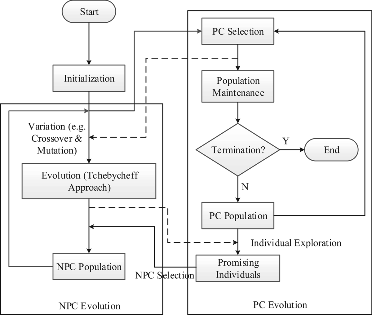
In ship collision avoidance path planning, we should consider not only safety among ships but also whether the planned ship collision avoidance trajectory is reasonable, that is, whether the length and smoothness of the path meet the physiological requirements of maritime personnel. Therefore, the planning of a ship collision avoidance trajectory should be regarded as a multi-objective problem so that the optimal solution set can provide reasonable choices for maritime personnel. In this paper, because a complex situation involving multi-ship encounters may result in a non-continuous Pareto-optimal front, we adopt Li's BCE framework for the Pareto criterion (PC) and non-Pareto criterion (NPC), which encompasses the advantages of the PC and NPC (Li et al., Reference Li, Yang and Liu2016). BCE is mainly divided into two parts: NPC evolution and PC evolution, and this approach can work with any non-Pareto evolutionary multi-objective optimisation (EMO) algorithm. In this paper, the MOEA/D (multi-objective evolutionary algorithm based on decomposition) algorithm is taken as the evolution part of the NPC, and the PC evolution part mainly uses the PC to select the relevant solution set. This method can overcome the poor convergence of PC evolution and the selection pressure of NPC evolution (Li et al., Reference Li, Yang and Liu2016). The PC evolution process mainly finds the Pareto-optimal solution set and maintains the original population size. The NPC evolution process is consistent with that of the NPC algorithm framework shown in Figure 6.

Figure 6. Procedure for BCE.
The key to the complementary advantages of NPC and PC in BCE lies in the selection of promising individuals based on the PC. Promising individuals are mainly non-dominated solutions of unselected or unexplored regions in the population of the NPC. The selection criterion for promising individuals is as follows: there are no NPC individuals or only one NPC individual in the niche range of non-dominated individuals in the PC population. Obviously, such a constraint avoids exploration of undeveloped and low-density regions in the NPC evolution.
The NPC evolution is based on the Tchebycheff approach of the MOEA/D algorithm. In this paper, considering that the evolution of the NPC is closely related to its neighbours and that the BCE algorithm communicates non-dominant individuals of PC evolution with NPC population, the ant lion algorithm is used here to update the population and improve individual crossover in NPC evolution. The ant lion algorithm is a novel nature-inspired algorithm that was proposed by Mirjalili based on the process of an ant lion preying on ants in nature (Mirjalili, Reference Mirjalili2015). In the population updating scheme of the ant lion algorithm, the elite ant lion and a random ant lion are taken as the centre ants, and the ants around them conduct a random walk to generate individuals. In the multi-objective algorithm, the elite ant lion is selected as the non-dominated solution, so the population updating process is directional. Therefore, according to the characteristics of population updating with the ant lion algorithm, the population updating strategy in BCE is improved to produce a better solution than those of traditional methods.
In this paper, because the NPC part of the BCE uses the MOEA/D algorithm, a random ant in the updated population is randomly selected from the neighbours. Because part of the initial population of PC evolution comes from the population generated by NPC evolution, the non-dominated solutions obtained from PC evolution are used in NPC evolution to determine whether there are non-dominated solutions among the neighbours of the currently updated individuals. If a solution exists, it may be randomly selected as an elite ant lion. If no solution exists, the elite ant lion randomly chooses among its neighbours. The new individual is as follows:
 $$\mbox{Ant}_j^t =\frac{R_A^h +R_E^h }{2}$$
 where  $\mbox{Ant}_{j}^{t} $ is the jth ant obtained from the hth iteration,
  $R_{A}^{h} $ is the solution obtained by randomly walking around a random ant lion, and
  $R_{E}^{h} $ is the solution obtained by randomly walking around the elite ant lion. The updating process in the ant lion algorithm is used to replace the cross-operations and improve the solution. Additionally, the mutation operation adopted is polynomial mutation (Wang et al., Reference Wang, Li and Li2018). In this manner, the above four variables representing the entire collision avoidance trajectory are taken as the targets of algorithm optimisation, and the desired solution of the collision avoidance trajectory is obtained based on an objective function that safety and costs.
3.2. The objective function
In the process of planning the avoidance trajectory, a ship should consider the safety among ships and the economics of the collision avoidance trajectory. Therefore, two objective functions for security and economy are adopted to reflect the quality of the solution obtained by the BCE algorithm in this paper. The VO algorithm is combined with the ship domain to construct a method of assessing the corresponding risk, and this method is applied to calculate the risk among ships with the following safety objective function:
 $$F_{{\rm safe}} =\mbox{Risk}_M$$
Therefore, the range of the safety objective function F safe is [0, 1], where RiskM is the maximum value of the collision risk at the avoidance point, restoration point and return point.
For the economic objective function, the general considerations are the time of the voyage, the length of the path and the fuel consumption of the voyage. Because collision avoidance planning occurs over a very short period compared with the time it takes to complete an entire route, it is not a good choice to consider the fuel consumption problem in collision avoidance. Therefore, treating the sailing time and sailing distance of a ship as linear variables, the path length of ship collision avoidance is taken as the economic objective function:
 $$F_{{\rm economy}} =\sum_k {\sqrt {( {x_{k+1} -x_k }) ^2+( {y_{k+1} -y_k } ) ^2} }$$
where F economy represents the distance between the initial point and the return point, as shown in Figure 4, (x, y) are the coordinates of the ship, and k is the index of the position of a ship at each time. The navigation simulation is carried out through the aforementioned ship motion mathematical model. In this paper, we choose the solution according to the range of the safety objective function, that is, a solution is randomly selected in the solution set with the value of F safe in the range of [0 · 2, 0 · 5) (Li et al., Reference Li, Wang and Zhao2019).
3.3. Hypothesis for collision avoidance
In a multi-ship collision avoidance plan, if it is determined that the ship will collide with another ship, the ships communicate with each other to clarify their respective sailing intentions. Here, the provisions of the International Regulations for Preventing Collisions at Sea 1972 (COLREGS) are used to judge the direction of ship actions (Rule 13, 14, 15). The TS with the greatest risk is evaluated based on the degree of danger, and the ship is steered based on the encountered situation involving the TS and another ship. If it is determined that the OS is the stand-on ship, the OS's steering is judged according to the encounter situation between the second dangerous ship and the OS, and so on, until the OS is found to give way. Alternatively, if all the TSs are judged and the OS is still the stand-on ship, and then the OS will not carry out the avoidance plan. Considering that the speed of the ship during the large angle steering (60°–80°) will decrease, the return range C a is limited to below 60 degrees.
According to the sailing intention of each ship, the multi-objective algorithm is used to plan each ship's avoidance route, and the improvement degree of this route relative to the original course is calculated. Through the communication between ships regarding their respective route improvements, the ship with the greatest improvement sails along the avoidance route. Other ships maintain their original routes, enter the next cycle, and again perform collision avoidance planning. This process continues until there is no risk of collision between ships. Taking into account the communication events and the run time of the algorithm, the time step is set to 3 min. After reaching the 3-min threshold, the ship will sail along the route planned in the cycle and enter the next time step. Since the ship domain itself takes into account the length of the ship, the ship is considered as a point, and the location of the point is the centre of the ship. The simulation program is MATLAB 2016b.
4. CASE STUDY
4.1. Four-ship encounter – situation 1 (mainly for crossing and head-on encounters)
In this scenario, the encounters between ships are dominated by crossing encounters and head-on encounters, as shown in Figure 7(a). The respective parameter information for the ships is shown in Table 2. In judging whether OS is the stand-on ship or the give-way ship, according to COLREGS, as long as a TS requires OS to give way, then the state of OS is the give-way ship. Therefore, when assessing the state of S 2, although the risk associated with S 1 is the greatest, according to COLREGS, S 2 is the stand-on ship, and the second-most-dangerous ship for S 2 is S 4. There is a crossing encounter between the two ships. Notably, S 4 is on the starboard side of S 2, and S 2 is the give-way ship. After the action status of each ship is defined, we use the BCE algorithm to plan the avoidance trajectory of each ship and calculate the route improvement degrees to identify the avoidance ship in the current cycle. The planned trajectory is shown in Figure 7(b), where the circle around the ship is the scope of the ship domain.

Figure 7. Multi-ship encounter situation (scenario 1) (left) and ship avoidance trajectories (right).
Table 2. Initial multi-ship encounter situation (crossing and head-on encounters).

The distance between the ships during collision avoidance is shown in Figure 8. The numbers on the lines in the figure represent the closest distance between ships in the collision avoidance trajectories (calculate the closest distance based on the centre point of the ship). The closest distance between the ships is greater than the radius of the ship domain on the side where the ships pass, which ensures that safety is maintained between the ships. In Figure 9, the ship navigation at the critical time node is illustrated. The presence of the ship domain around each ship rather than the expansion of the ship domain not only ensures safety but also avoids the unnecessary oversteering of the ship. Among them, S 1, S 2 and S 3 all turn to the starboard side, mainly according to COLREGS. Table 3 shows the trajectory improvement degree of each ship in each cycle. The order in which the ship collision avoidance trajectory is selected can be observed. The ship with a planned avoidance trajectory does not participate in avoidance planning in the next cycle, and the improvement degree is zero. The action ship in the first cycle is S 1, and the action ship in the second cycle is S 3, followed by S 2 in the third cycle. The collision avoidance parameters of these ships are shown in Table 3. Due to the avoidance behaviour of the first three ships, S 4 is not in danger at this time, so it maintains its original course. In this scenario, the avoidance of each ship will not generate new collisions, and the planning of the following ships will consider the avoidance of the previous ships so that all ships can sail safely.

Figure 8. Relative distance between ships.

Figure 9. Trajectory of each ship at given times.
Table 3. The value of ImpRS in each cycle.

4.2. Four-ship encounter – situation 2 (mainly for crossing and overtaking encounters)
In this scenario, an overtaking encounter situation is added, as shown in Figure 10(a). In Table 4, there is a danger of collision between S 4 and S 1, and the two ships experience a crossing encounter. Additionally, since the length of the ships is identical, the difference in ship speed leads to different sizes of the ship domain. The parameters of each ship are shown in Table 4. The trajectory of each ship after planning can be seen in Figure 10(b). S 1 and S 2 conducted avoidance operations, and S 3 and S 4 maintained their original courses. The ship avoidance and steering manoeuvres were in accordance with COLREGS.

Figure 10. Multi-ship encounter situation: scenario 2 (left) and ship avoidance trajectories (right).
Table 4. Initial multi-ship encounter situation (crossing and overtaking encounters).

The distance between the ships in each voyage is shown in Figure 11, and the numbers on the lines indicate the closest distance between the ships (calculate the closest distance based on the centre point of the ship). The closest distance between the ships is greater than the radius of the ship domain on the side where the ship passes. For S 3 and S 4, in Figure 10(b), both ships are sailing based on their original headings. In addition, in Figure 12, at 900 s, S 3 and S 4 pass on the starboard side. The minimum distance between the two ships is 854·6 m, which is greater than the starboard radius of the two ships. Thus, it is safe for the ships to pass at that distance. Figure 12 shows the navigation status of the ships at each point in time. In Table 5, we can see the improvement degree of each ship in each time cycle and the avoidance action for that cycle. The avoidance parameter values of each ship are shown in Table 5.

Figure 11. Relative distance between ships.

Figure 12. Trajectory of each ship at given times.
Table 5. The value of ImpRS in each cycle.

4.3. Multi-ship and static obstacle encounters
Static obstacles are introduced in this scene. Considering the convenience in the algorithm, obstacles are assigned circular shapes, as shown in Figure 13(a). And the parameters of each ship are shown in Table 6. Here, the radius of the static obstacle is set to 1180 m, which can be regarded as a stationary ship or buoy not considered in the navigation plan. The avoidance trajectory of each ship is shown in Figure 13(b). In considering the ship avoidance direction for static obstacles, only the direction of the minimum steering amplitude is considered here to determine which direction to turn the ship, port or starboard. In avoidance steering tasks, the requirements of COLREGS are still considered.

Figure 13. Multi-ship and static obstacle encounter situation (scenario 3) (left) and ship avoidance trajectories (right).
Table 6. Initial multi-ship and static obstacle encounter situation.

Figure 14 shows the distance between the ships during their voyages (calculate the closest distance based on the centre point of the ship). As shown, the distance between each ship and the static obstacle is greater than each ship domain radius. In Figure 15, the navigation status of the ship is used in each time period. At 1,000 s, S 1 and S 3 pass on their respective port sides. In Figure 14, the closest distance between the two ships is 1144·8 m, which is greater than the port radius of their respective ship domains, so they are safe from colliding. At 1,400 s, S 1 and S 2 pass on their respective port sides. In Figure 14, the closest distance between the two ships is 1530·2 m, which is greater than the radius on the port side of each ship domain. Then, the ships complete their avoidance operations and return to their original routes to continue sailing. Table 7 shows the improved values for each ship in each time cycle. Because S 4 is a static obstacle, it does not need to be planned, and the corresponding value is zero.

Figure 14. Relative distance between ships.

Figure 15. Trajectory of each ship at given times.
Table 7. The value of ImpRS in each cycle.

4.4. Computing time of the algorithm
The calculation time of the collision avoidance method and the time of constructing the VO area are shown in Figure 16. Among them, the horizontal ordinate N represents the number of obstacles and the running time of the program in the longitudinal coordinates. In Figure 16 (left), it can be observed that the time to construct the VO area is related to the number of obstacles. In Figure 16 (right), it is about the time of one-time collision avoidance algorithm planning for a ship. Because this paper adopts a multi-objective algorithm, assuming that the number of iterations is M and the number of population is P, the time complexity of the algorithm is generally O(MP). From Figure 16, it can be observed that the time curve of constructing the VO zone is basically consistent with the trend of running time of the program, that is to say, the main time-consuming part of the whole algorithm is the calculation of the collision risk. At the same time, it can be observed from the figure that the running time of the algorithm increases linearly with the number of obstacles. It can be observed from the figure that the calculation time of one cycle program is 7·51 s in the case of six ships (i.e. five obstacles). Since one ship does not plan collision avoidance for the next time in each cycle, the normal time for six ships to plan each other's trajectories is 24·66 s (i.e. adding up the data in the figure). Therefore, the collision avoidance method proposed in this paper can operate normally in a general multi-ship environment.

Figure 16. Construction time of VO area (left) and running time of multi-objective algorithm (right).
5. CONCLUSIONS
This paper mainly studies the problem of ship collision avoidance path planning in the case of multi-ship encounters and the existence of dynamic ships and static obstacles. BCE is used to plan the entire collision avoidance trajectory; that is, the entire trajectory is considered based on four parameters: T o, C o, T a and C a. In this approach, although the communication times of this method are consistent with those of the DLSA algorithm in each cycle, the number of communication times will be greatly reduced from the point of view of the entire planning process. This paper combines the ship domain with the VO method to assess potential collisions. Based on this method, a new method of calculating the risk between ships is proposed. Additionally, a new ant lion algorithm concept is added to NPC evolution to enhance the convergence of the method. Based on the steering amplitude, the reduction of risk and the time information for a collision avoidance trajectory, a new improvement function considering safety and efficiency is proposed. The improvement function is applied to select the avoidance action ship in each cycle.
Although this method can achieve good results, there are some drawbacks. For example, we do not consider the problem of velocity variation during ship turning. Moreover, we need to consider the collision avoidance planning problem with uncooperative ships, which would include trajectory prediction. In addition, this paper does not consider speed collision avoidance and the collision avoidance operation requires both a speed change and a course change, or consider multiple collision avoidance behaviour, such as multiple static obstacles environment, so as to obtain the optimal solution.
Supplementary material
The supplementary material for this article can be found at https://doi.org/10.1017/S0373463320000053