1. INTRODUCTION
The Closest Point of Approach (CPA) is an estimated point at which the distance between the own ship and another object target will reach the minimum value. CPA is a valuable quantity in assessing ship safety with regards collision avoidance. CPA is presented in Automatic Radar Plotting Aids (ARPA) to assist in direct estimation of collision risk. CPA consists of two parameters: the Distance at Closest Point of Approach (DCPA) and the Time to Closest Point at Approach (TCPA). These should be obtained by the ship officer on target vessels in order to determine whether the risk of collision exists (Bole et al., Reference Bole, Wall and Norris2014). A ship officer then makes the collision avoidance decision taking into account the manoeuvring characteristics of the ship, the tactical situation (course, speed and aspect of target vessels) and the DCPA/TCPA. Furthermore, the CPA may be considered in judging the responsibility of the involved ships in a maritime accident investigation.
Figure 1 (left) shows two ships: ship A and ship B. Over the time series t 1, t 2, t 3, t 4 and t 5, ship A navigates from A 1 to A 5 following a straight trajectory, while ship B navigates from B 1 to B 5 also linearly. Suppose ship A is the own ship and considered as the relative object. The relative motion of the object ship (ship B) is illustrated in Figure 1 (right). Based on both the initial positions and the true velocity vectors of ship A and ship B, the CPA can then be obtained (Sameshima, Reference Sameshima1961).
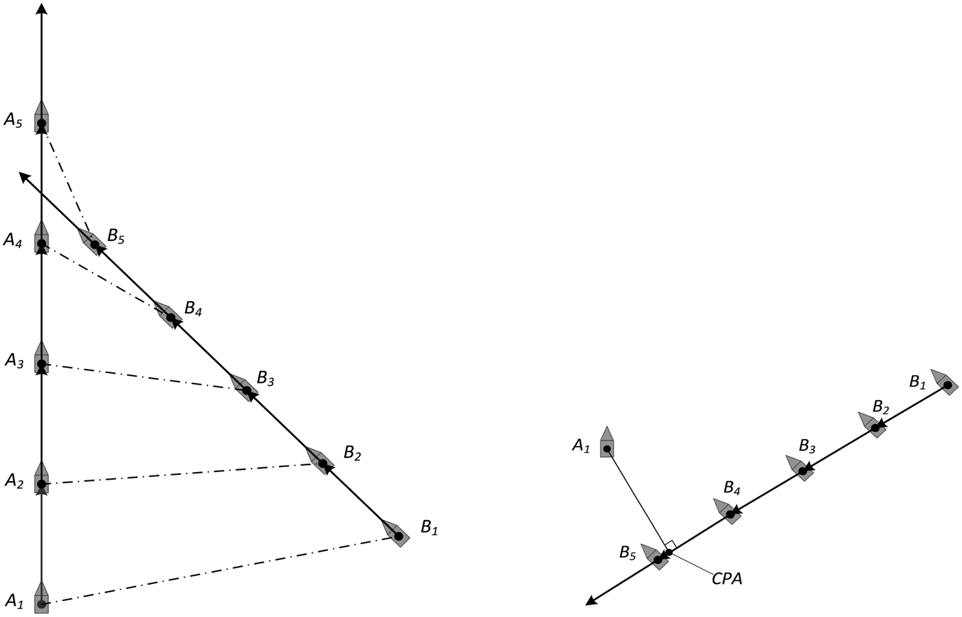
Figure 1. A situation of ships approaching each other.
As a crucial factor for collision avoidance, CPA is widely used in the maritime industry to obtain the ship domain and assess the navigational risk. CPA was originally introduced when radar was first used to avoid the collision. Radar is an essential safety facility also used by aircraft and other systems. CPA is therefore not only useful for ship safety, but also helpful for aircraft collision avoidance (Kim et al., Reference Kim, Lee, Lee and Kang2013) and vehicles (Huang and Lin, Reference Huang and Lin2012). Pimontel (Reference Pimontel2007) looked at the factors that might affect CPA and suggested that there were no clear relationships between the vessel type and CPA, between the vessel dimension and CPA, or between the vessel speed and CPA. However, the correlations of CPA with the size, speed and course of the ship were studied by Mou et al. (Reference Mou, Tak and Ligteringen2010) with regard to linear regression models. These models were then developed to present a dynamic method for assessing the risk.
Jeong et al. (Reference Jeong, Park and Kim2013) used radar and AIS data to assess the safety of vessels. The analysed DCPAs of assessed ships were less than one mile when crossing the Mokpo-Gu waterway. The distribution of CPAs was analysed geographically to show the special regions of traffic intensity, the risk in the waterway and patterns of marine traffic.
To assist the pilot in decision-making in close-quarters situations, Chin and Debnath (Reference Chin and Debnath2009) built a model to perceive the collision risk in port waters based on CPA. In the regression model, TCPA and DCPA were two key factors in computing the collision risk. As a case study, the risks perceived by Singapore port pilots were obtained to calibrate the regression model. This model could be used to give a better understanding of the collision risk and define a more appropriate level of evasive actions.
A risk model consisting of four risk levels, based on the Convention on International Regulations for Preventing Collisions at Sea (COLREGs), was built by Hilgert and Baldauf (Reference Hilgert and Baldauf1997). The actual value of CPA, the actual distance between involved ships in an encounter situation, and identified limit values were needed for the application of the risk model.
Choi et al. (Reference Choi, Kim, Lee and Kim2013a) developed a real-time collision avoidance algorithm for unmanned aerial vehicles. This algorithm was based on the geometry of CPA and a collision detection/resolution scheme. Mathematical equations for calculating the algorithm based on the single vision detector were discussed by Choi et al. (Reference Choi, Kim and Hwang2013b).
The CPA calculation method as above is widely adopted for collision avoidance research. In this traditional method, each of the involved ships is assumed to navigate in a straight trajectory with a certain velocity vector. This can present DCPA and TCPA directly as each approaching ship will navigate ahead with a constant Speed Over Ground (SOG) and a constant Course Over Ground (COG). Actually the ship may change or intend to change the course or speed when approaching. The traditional method therefore lacks accuracy if a ship is changing speed or turning. SOG, COG, the Change Of Speed (COS) and the Rate Of Turn (ROT) are the essential dynamic factors for the ship motion.
With the situation as in Figure 1 at the time t 1, consider if ship B is changing course with a certain ROT at position B 1. The trajectory of ship B will be a curved trajectory rather than a straight line, as shown in Figure 2 (left). Obviously, the approaching situation significantly differs from the prior situation shown in Figure 1. Traditional DCPA and TCPA cannot support the collision avoidance decision effectively. Actions to avoid collision may then have less or no effect, may prove to be a waste of time/fuel and, sometimes even lead to a higher risk of collision. The same can also be shown in Figure 2 (right) if the speed of ship B is changing.

Figure 2. Situations of approaching with a ROT/COS of ship B.
Therefore, a new method taking into account SOG, COG, COS and ROT needs to be developed. Ship positions need to be predicted more accurately by using these four key factors. CPA computed by these predicted positions is more supportive of collision avoidance planning.
2. SHIP TRAJECTORY PREDICTION METHOD
2.1. AIS data
AIS can be used to provide all information of the required four factors. SOG and COG are provided in all AIS systems. For Class A AIS information, ROT is additionally provided as a separate data field derived from the ship equipment. For Class B AIS information, ROT is not transmitted but can be estimated by the COG changes from the last two AIS reports. COS can be estimated from SOG changes as well.
To obtain predicted positions for use by a shore-based operator, the derived COS and ROT should be first obtained from the last received AIS messages (as described in Section 2.2). The future positions of a ship can then be predicted by applying: (1) the derived COS and ROT, and (2) SOG and COG from the last AIS positions (as described in Section 2.3). In the case of Class A AIS vessels, the ROT will not need to be derived from the recent past positions, but can be computed to check whether the received ROT information is correct.
According to the requirements of the International Telecommunication Union (ITU), AIS information is periodically transmitted at variable intervals depending on the navigation status of the ship and the type of AIS (ITU, 2014).
Future predictions of SOG and COG can be prepared by smoothing AIS data from two or more AIS messages. Future COS and ROT can be obtained from the predicted SOG and COG. The more points used, the better the theoretical accuracy. However, if going back in time for more than a couple of minutes, the data may be misleading with the ship having performed more than one manoeuvre in that time interval. In the case of small fast vessels, even a period of two minutes is sometimes too long. Consequently the prediction period depends on the type of the case ship. Since this method is developed for typical cargo and conventional passenger vessels, a period of three minutes is sufficient for the prediction.
2.2. SOG and COG prediction
2.2.1. Exponential smoothing model
The exponential smoothing model was firstly proposed by Holt (Reference Holt2004). This model can use periodic time series data to obtain smoothing data or to predict future data. When the ship is navigating in a waterway with an approximately steady speed, AIS data is broadcast with a certain periodicity, so that the data can be viewed as periodic time series data.
Set the real value as x, the predicted value as s, and the order of the period as t, t ≥ 1. The simplest form of this method is the single exponential smoothing model:
 $$\left\{ \matrix{s_1 = x_0\; \hfill \cr s_{t + 1} = \alpha x_t + \left( {1 - \alpha } \right)s_t \hfill} \right.\,t \ge 1$$
where α is the weight factor, α ∈ [0, 1], s 1 is initialised to x 0 (this initial value can also be set by other methods, such as the mean of previous several values of x), and s t+1 is the first smoothing value after the real value x t .
Two more models commonly used are the double exponential smoothing method and the triple exponential smoothing method, which have equations developed from the above model. In this paper the triple exponential smoothing method is chosen to predict SOG and COG because a ship may change or intend to change its SOG or COG at any time. This method is more applicable in these circumstances. The triple exponential smoothing model is described as follows (Winters, Reference Winters1960; American National Institute of Standards and Technology, 2012):
 $$\left\{ \matrix{{s}^{\prime}_{t} = \alpha \cdot x_t + \left( {1 - \alpha } \right){s}^{\prime}_{t - 1} \hfill \cr {s}^{\prime \prime}_{t} = \alpha \cdot {s}^{\prime}_{t} + \left( {1 - \alpha } \right){s}^{\prime \prime}_{t - 1} \hfill \cr {s}^{\prime \prime \prime}_{t} = \alpha \cdot {s}^{\prime \prime}_{t} + \left( {1 - \alpha } \right){s}^{\prime \prime \prime}_{t - 1} \hfill \cr a_t = 3{s}^{\prime}_{t} - 3{s}^{\prime \prime}_{t} + {s}^{\prime \prime \prime}_{t} \hfill \cr b_t = \displaystyle{{\alpha ^2} \over {2{\left( {1 - \alpha } \right)}^2}}\left[ {\left( {6 - 5\alpha } \right){s}^{\prime}_{t} - \left( {10 - 8\alpha } \right){s}^{\prime \prime}_{t} + \left( {4 - 3\alpha } \right){s}^{\prime \prime \prime}_{t}} \right] \hfill \cr c_t = \displaystyle{{\alpha ^2} \over {{\left( {1 - \alpha } \right)}^2}}\left( {{s}^{\prime}_{t} - 2{s}^{\prime \prime}_{t} + {s}^{\prime \prime \prime}_{t}} \right) \hfill \cr F_{t\left( m \right)} = a_t + mb_t + \displaystyle{1 \over 2}m^2c_t\; \hfill} \right.$$
where t is the current time and t ≥ 2, α is the weight factor and α ∈ [0, 1], x t is the real value at the current time, s′ t−1 is the single smoothing value at the time t − 1 at which it can be initialised to x t−1, s′ t is the single smoothing value at the time t, s″ t−1 is the double smoothing value at the time t − 1 which can be initialised to x t−1, s″ t is the double smoothing value at the time t, s″′ t−1 is the triple smoothing value at the time t − 1 which can be initialised to x t−1, s″′ t is the triple smoothing value at the time t, m is the number of the predicted values and F t(m) is the m th predicted value at the time t.
2.2.2. SOG and COG prediction
Suppose there is a sequential SOG with the value v n where n is the ordinal number. One is added to the ordinal number when the next data is received.
Based on Equation (2), the prediction method can start to work when two sequential AIS data messages are received. At this time, the initial single smoothing value, the double smoothing value and the triple smoothing value can all be initially set as v n−1. The first series of the predicted SOG values with the same time interval can be obtained based on the last value v n−1 and the current value v n .
Set v n(m) as the m th predicted SOG value whethe n th AIS message is received. The series of the predicted values of SOGs can be obtained by Equation (2):
 $$\left[ {v_{n\left( 1 \right)}, \; v_{n\left( 2 \right)}, \; v_{n\left( 3 \right)}, \cdots, v_{n\left( m \right)}} \right]$$
After a time interval, the ordinal number n has one added to it becoming n + 1, a new real AIS data message will be produced, broadcast, received and updated by the vessel. A new series of the predicted SOG values based on this new (n + 1)th AIS message can then be obtained.
The predicted COG values can be obtained by the same method as:
 $$\left[{c_{n\left( 1 \right)}, \; c_{n\left( 2 \right)}, \; c_{n\left( 3 \right)}, \cdots, c_{n\left( m \right)}} \right]$$
2.3. Position prediction based on the navigation features
The future positions of a ship are affected not only by SOG and COG, but also by COS and ROT. These four factors cannot be ignored, so the traditional prediction model (which only uses COG and SOG) is modified by taking into account COS and ROT to predict ship positions.
2.3.1. Prediction of the movement using the four factors
As shown in Figure 3, there exist two random sequential positions: [x k−1, y k−1] at the time t k−1 and [x k , y k ] at the time t k . The course c k−1 changes to c k correspondingly. The distance d between these two positions can be obtained as follows:
 $$d = \root 2 \of {\left( {dx} \right)^2 + \left( {dy} \right)^2} $$
where dx is the horizontal movement and dy is the vertical movement.
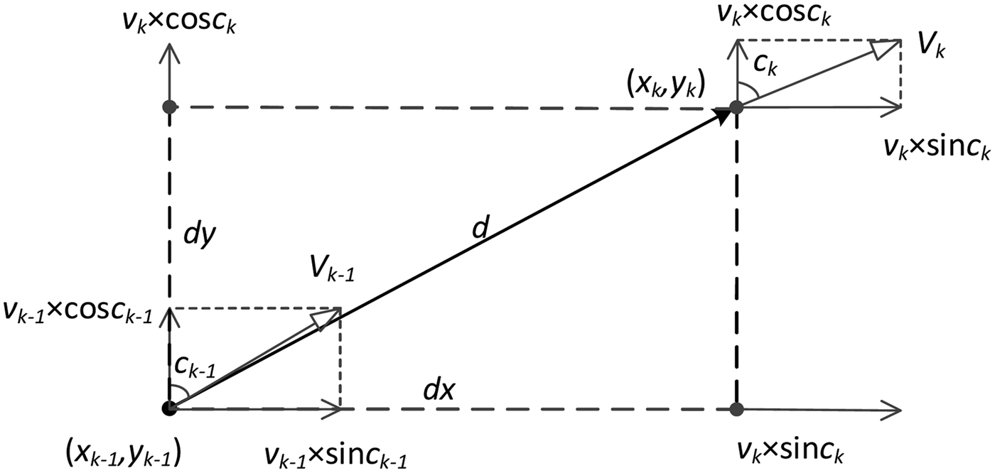
Figure 3. Distance between any two continuous positions.
The COS value c and ROT value r during this period from t k−1 to t k can be obtained as follows:
 $$\left\{ {\matrix{ {c_{k - 1} = \displaystyle{{v_k - v_{k - 1}} \over {t_k - t_{k - 1}}}} \cr {r_{k - 1} = \displaystyle{{c_k - c_{k - 1}} \over {t_k - t_{k - 1}}}} \cr}} \right.$$
If the target vessel uses a Class A AIS, a value of r should be available from the target ship.
As shown in Figure 3, at any point [x t , y t ] between [x k−1, y k−1] and [x k , y k ], the horizontal speed and the vertical speed are as follows:
 $$\left\{ {\matrix{ {v_x = \left[ {v_{k - 1} + c_{k - 1} \left( {t - t_{k - 1}} \right)} \right] {\rm sin} \left[ {c_{k - 1} + r_{k - 1} \left( {t - t_{k - 1}} \right)} \right]} \cr {v_y = \left[ {v_{k - 1} + c_{k - 1} \left( {t - t_{k - 1}} \right)} \right] {\rm cos} \left[ {c_{k - 1} + r_{k - 1} \left( {t - t_{k - 1}} \right)} \right]} \cr}} \right.$$
The horizontal movement dx is the integral of v x and the vertical movement dy is the integral of v y , the movements can then be obtained by the following equations:
 $$\left\{ \matrix{dx = \int_{t_{k - 1}} ^{t_k} {vx\,dt} \hfill \cr dy = \int_{t_{k - 1}} ^{t_k} {vy\,dt} \hfill} \right.$$
According to Equations (5) and (6), there exist:
 $$\left\{ \matrix{dx = \int_{t_{k - 1}} ^{t_k} {\left[ {v_{k - 1} + \left( {v_k - v_{k - 1}} \right)\displaystyle{{t - t_{k - 1}} \over {t_k - t_{k - 1}}}} \right]} \,{\rm sin}\,\left[ {c_{k - 1} + \left( {c_k - c_{k - 1}} \right)\displaystyle{{t - t_{k - 1}} \over {t_k - t_{k - 1}}}} \right]dt \hfill \cr dy = \int_{t_{k - 1}} ^{t_k} {\left[ {v_{k - 1} + \left( {v_k - v_{k - 1}} \right)\displaystyle{{t - t_{k - 1}} \over {t_k - t_{k - 1}}}} \right]\,{\rm cos}\,\left[ {c_{k - 1} + \left( {c_k - c_{k - 1}} \right)\displaystyle{{t - t_{k - 1}} \over {t_k - t_{k - 1}}}} \right]dt} \hfill} \right.$$
At the initial time t 0, the ship is navigating at the position [x 0, y 0] with the SOG value v 0 and COG value c 0. Set the time interval as Δt, t n = t 0 + n × Δt. At the time t n , SOG is set as v n , while COG is set as c n .
SOGs and COGs of the future positions can be predicted based on Equation (2). Suppose m predicted SOGs and m predicted COGs are obtained as [v n(1), v n(2), v n(3), · · · , v n(m)] and [c n(1), c n(2), c n(3), · · · , c n(m)], respectively.
At the time t n , based on Equation (7), the distances of the ship movement between position [x n , y n ] and the m th predicted position at the horizontal axis and the vertical axis can be calculated as follows:
 $$\left\{ \matrix{dx_{n\left( m \right)} = \sum\limits_{k = 1}^m {\int_{t_{k - 1}} ^{t_k} {\left[ {v_{k - 1} + \left( {v_k - v_{k - 1}} \right)\displaystyle{{t - t_{k - 1}} \over {t_k - t_{k - 1}}}} \right]{\rm sin}\left[ {c_{k - 1} + \left( {c_k - c_{k - 1}} \right)\displaystyle{{t - t_{k - 1}} \over {t_k - t_{k - 1}}}} \right]dt}} \hfill \cr dy_{n\left( m \right)} = \sum\limits_{k = 1}^m {\int_{t_{k - 1}} ^{t_k} {\left[ {v_{k - 1} + \left( {v_k - v_{k - 1}} \right)\displaystyle{{t - t_{k - 1}} \over {t_k - t_{k - 1}}}} \right]{\rm cos}\left[ {c_{k - 1} + \left( {c_k - c_{k - 1}} \right)\displaystyle{{t - t_{k - 1}} \over {t_k - t_{k - 1}}}} \right]dt}} \hfill} \right.$$
where k is the ordinal number of the ship position among m predicted positions, 2 ≤ k ≤ m, dx n(m) is the horizontal distance between position [x n , y n ] and the m th predicted position, dy n(m) is the vertical distance between the position [x n , y n ] and the m th predicted position, v n(k) is the k th predicted SOG value when the current time is t n , and c n(k) is the k th predicted COG value when the current time is t n .
The distance between position [x n , y n ] and the m th predicted position can then be obtained by Equations (3) and (8).
2.3.2. Prediction of ship positions
At the time t n , the moving distances at the horizontal axis and vertical axis between the current position [x n , y n ] and the m th predicted position can be obtained. The m th predicted position [P m lat n , P m lon n ] can then be obtained by converting the distances to longitude and latitude (Veness, Reference Veness2012):
 $$\left\{ \matrix{P_m lat_n = {\rm arcsin}\left[ {sin \left( {y_n} \right) \times cos\displaystyle{{d_{n\left( m \right)}} \over R} + \left. {\displaystyle{{dx_{n\left( m \right)}} \over {d_{n\left( m \right)}}} \times cos\left( {y_n} \right) \times sin\displaystyle{{d_{n\left( m \right)}} \over R}} \right]} \right. \hfill \cr P_m lon_n = x_n + {\rm arctan}\left[ {\displaystyle{{\displaystyle{{dy_{n\left( m \right)}} \over {d_{n\left( m \right)}}} \times {\rm sin}\displaystyle{{d_{n\left( m \right)}} \over R} \times {\rm cos}\left( {y_n} \right)} \over {{\rm cos}\displaystyle{{d_{n\left( m \right)}} \over R} \times {\rm sin}\left( {y_n} \right) \times \sin \left( {P_m lat_n} \right)}}} \right] \hfill} \right.$$
where P m lat n is the predicted m th latitude at the time t n , P m lon n is the predicted m th longitude at the time t n , d n(m) is the moving distance obtained by dx n(m) and dy n(m) based on Equation (3) and R is the radius of the Earth.
It is worth noting that the Earth is assumed as a sphere in order to simplify the calculation process.
The series of predicted positions can then be obtained as:
 $$P_n = \left[ {\matrix{ {P_1 lat_n, \; P_2 lat_n, \; P_3 lat_n, \cdots, P_m lat_n} \cr {P_1 lon_n, \; P_2 lon_n, \; P_3 lon_n, \cdots, P_m lon_n} \cr}} \right]$$
3. CPA CALCULATION
3.1. Asynchronous AIS positions
After the ship positions are predicted, the new trajectory of the ship can be obtained differing from the normally predicted linear trajectory. Each ship has a new predicted trajectory. The CPAs need to be calculated as accurately as possible to estimate the probability of collision.
However, according to the requirements of ITU, AIS is not continuously transmitted but at intervals (ITU, 2014). Therefore the AIS data received from different ships is asynchronous. When a ship is underway, the AIS data usually has an interval of 30 seconds between positions from each Class B AIS, and has an interval of 10 seconds between positions from each Class A AIS.
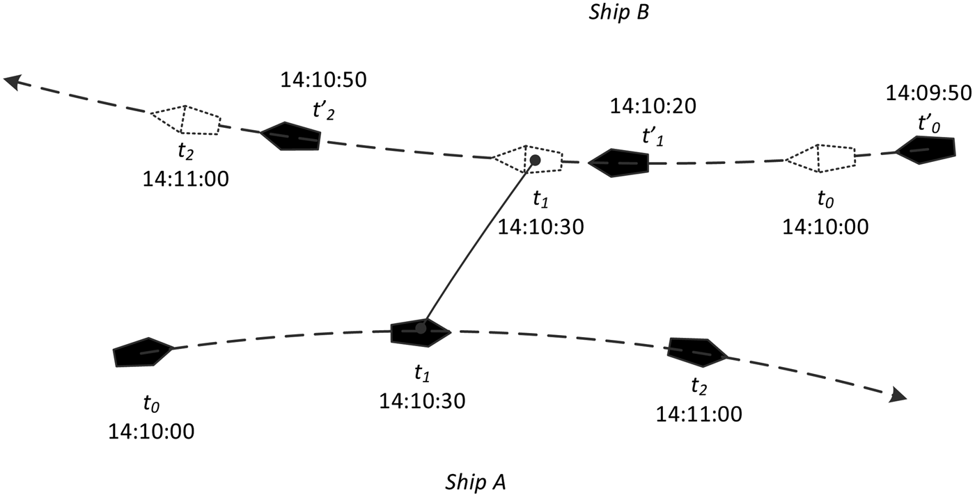
Figure 4 shows two ships. When the shore observer obtains the latest positions of ship A at the time t 0, t 1 and t 2, the received positions of ship B are at the time t′0, t′1 and t′2 before t 0, t 1 and t 2 respectively (t′0 < t 0 < t′1 < t 1 < t′2 < t 2). Consequently, the CPA cannot be obtained directly until the position data is synchronised.
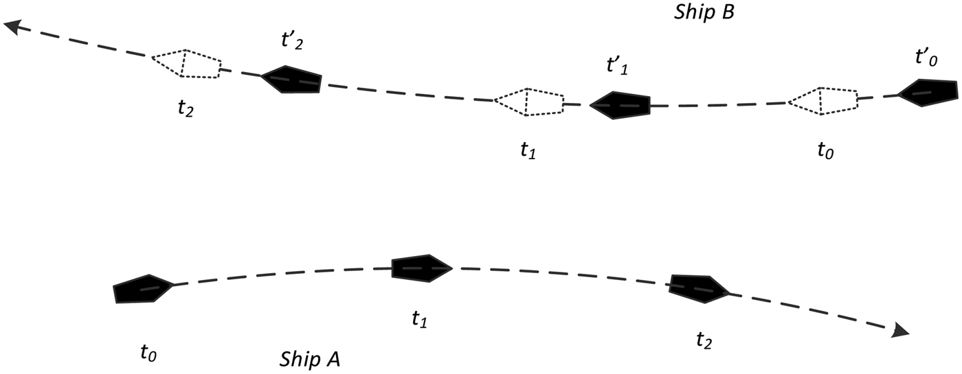
Figure 4. Asynchronous AIS positions.
3.2. CPA calculation
An efficient CPA calculation method using the asynchronous series of data is proposed in this section. Firstly, the hill climbing algorithm is described. This is used to choose a closest approaching position among the predicted positions which have varying time intervals. Secondly, the theory of the golden section search algorithm is explained. The details of the methodology which uses these two techniques to obtain the final CPA are provided later.
3.2.1. Hill climbing algorithm
Suppose the target function of the distance between two ships is f(t), t is a vector of continuous or discrete time values. If the mathematical description of f(t) is not given, the hill climbing algorithm can be used to attempt to minimise the distance function f(t) by adjusting the time value of t.
At each iteration, the hill climbing adjusts t and determines whether the change improves the distance function f(t). With the hill climbing algorithm, any change that improves f(t) is accepted if the change of distance satisfies:
 $$d\;f\left( t \right) \lt 0$$
If the distance change d f(t) > 0, it means that the distance function f(t) starts to increase, and the previous distance is smaller. The hill climbing should then be stopped. If d f(t) = 0, it means that the change of t cannot improve the distance function. However the improvement of the next function f(t) is still unknown. The hill climbing should then be carried on. The iteration therefore should continue until d f(t) changes from d f(t) ≤ 0 to d f(t) > 0. The final adjusted t which follows d f(t) < 0 is the locally optimal solution (Storey, Reference Storey1962). If the change of distance d f(t) after this local optimal is equal to zero, the time t after this locally optimal solution is another locally optimal solution.
In CPA calculation processes, the hill climbing algorithm is used to find the shortest distance among all the pairs of the predicted positions of two approaching ships. The algorithm starts at the latest true AIS position and continues until the change of distance becomes positive (larger than zero).
3.2.2. Golden section search algorithm
The golden section search algorithm was presented by Kiefer (Reference Kiefer1953) to find the final minimum value of the distance function f(t) in this paper. This value will be the DCPA. By comparing the function value at the golden section ratio with a known value in the middle position, the range of time t can be narrowed constantly until a satisfactory result is found.
In the case shown in Figure 5, point e is the middle point of endpoints a and b, f(e) is the function value (distance) at point e, f(e) < f(a) and f(e) < f(b). To find the minimum of the distance function f(t) in the range [a, b], the distance value of f(g) is obtained using the golden section ratio g, where g follows g − a = 0·618(b − a). If f(g) > f(e), like the left-bottom of Figure 6, the function value in the range (g, b] is always larger than f(g). Therefore the minimum is not in the range (g, b]. The range is then narrowed from [a, b] to [a, g]. If f(g) < f(e), like the right-bottom of Figure 6, the function value in the range [a, e) is always larger than f(e). Therefore the range is narrowed to [e, b]. If f(g) = f(e), compute a new golden section ratio g following b − g = 0·618(b − a). Then repeat the comparison. The comparison is repeated with two values so as to narrow the range until a satisfactory result is found.
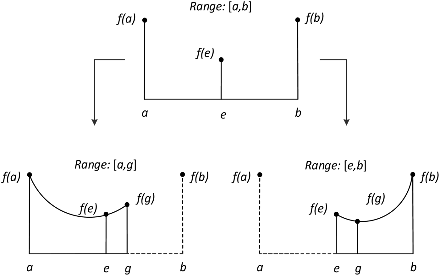
Figure 5. The basic method of golden section search.

Figure 6. Step 1: Example showing the up-CPA.
3.2.3. CPA calculation method
There are three steps to search the final CPA based initially on the asynchronous AIS positions. The first two steps aim at obtaining a position among predicted positions, the third step aims at obtaining the final CPA.
Step 1: Calculation of the unsynchronised-pseudo-CPA. Firstly, the distance between two ships can be calculated directly for comparison, in accordance with the positions of these two ships. If the positions of two ships are (lat 1, lon 1) and (lat 2, lon 2), the distance between them is obtained as follows:
 $$l = \arccos \left[ {\sin \left( {lat_1} \right)\sin \left( {lat_2} \right) + \cos \left( {lat_1} \right)\cos \left( {lat_2} \right){\rm cos}\left( {lon_1 - lon_2} \right)} \right] \times R$$
where l is the distance between the two positions and R is the radius of the Earth.
Calculate the distance l′ between two series of predicted positions of two approaching ships in order, using AIS message times which have the closest match. The hill climbing algorithm starts at the two first positions of the two ships. To obtain the shortest distance, it can be accepted if the change of distance d l′ is less than zero:
 $$d\;l^{\prime} \lt 0$$
If the change of distance d l′ is larger than zero, it means that the values of the obtained distance are increasing and the ships are moving away from each other, the closest predicted point of approach is the current position and can be referred to as the unsynchronised-pseudo-CPA (up-CPA), as shown in Figure 6.
Step 2: Calculation of the synchronised pseudo-CPA. Based on a predicted position which is obtained in Step 1 as the up-CPA, the corresponding position of the object ship at the same time can then be calculated by the cubic spline interpolation method (Hasberg et al., Reference Hasberg, Hensel, Westenkirchner and Bach2008; Sang et al., Reference Sang, Wall, Mao, Yan and Wang2015). The initial real distance l between these two positions can be calculated by Equation (12). The hill climbing algorithm can also be used in this step to find the real shortest distance among all the synchronised positions. The corresponding position of the approaching ship can be referred to as the synchronised pseudo-CPA (p-CPA) shown in Figure 7.

Figure 7. Step 2: The synchronised p-CPA in the example.
After the pair of the p-CPAs is obtained as above, it should be mentioned that this process must now be repeated to obtain two other real distances: (1) the real distance between the previous pair of positions of the two ships and, (2) the real distance between the next pair of positions. These two real distances will be used in Step 3.
Step 3: Calculation of the final CPA. The golden section search algorithm is used to obtain final CPAs of these two ships, based on the pair of the obtained p-CPAs, the previous pair of positions and the next pair of positions. The initial time range is from the time at the predicted position before the p-CPA position to the time at the predicted position after the p-CPA position. The corresponding distances are obtained in Step 2. Within this time range, the initial value of the middle time is the time at the p-CPA. The method as detailed in Section 3.2.2 is used to find the real CPA. When the range of the time interval is reduced to no more than one second, a DCPA l is then found. The final CPA is just at the last golden section ratio point as shown in Figure 8.
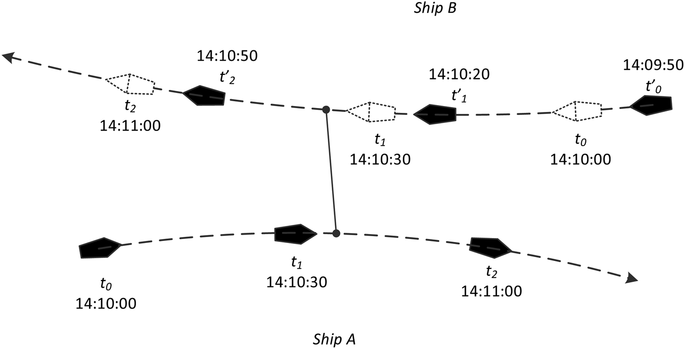
Figure 8. Step 3: The final CPA in the example.
Since the received AIS positions of approaching ships are actually the positions of AIS antennae, the calculation of the real DCPA l r should take more factors into account based on the obtained DCPA l. As shown in Figure 9, once CPAs are obtained, the relative bearing γ of the approaching ship can then be obtained according to the line connected by CPAs and the heading information of the own ship. It should be noted that: (1) the heading information can be extracted from Class A AIS directly and, (2) for Class B AIS, the heading information can be obtained by other nautical sensors, such as the gyrocompass. Meanwhile, when a ship is fitted with AIS, the position of the AIS antenna should be located by parameters d 1, d 2, d 3 and d 4. d 1 and d 2 are the perpendicular distances from the AIS antenna to the bow and the stern of ship, respectively. In addition, d 3 and d 4 are the perpendicular distances from the AIS antenna to the portside and starboard side, respectively. These parameters are broadcast as static information.
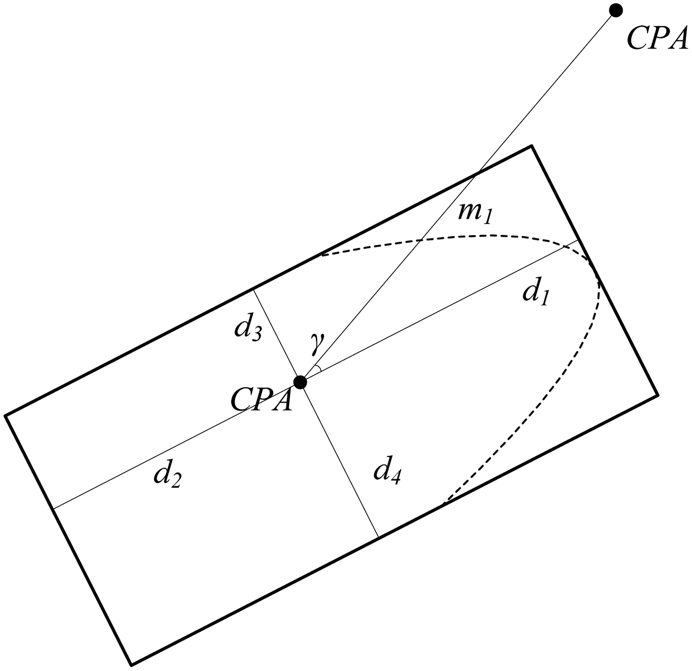
Figure 9. Diagram of DCPA calculation.
The overlap distance m 1 can be approximately computed as follows:
 $$m_1 = \left\{ {\matrix{ {\displaystyle{{d_1} \over {{\rm cos}\gamma}}} & {\gamma \in \left[ {{\rm - arctan}\displaystyle{{d_3} \over {d_1}}, {\rm arctan}\displaystyle{{d_4} \over {d_1}}} \right]} \cr {\displaystyle{{d_4} \over {\cos \left( {0.5\pi - \gamma} \right)}}} & {\; \; \gamma \in \left[ {{\rm arctan}\displaystyle{{d_4} \over {d_1}}, \pi - {\rm arctan}\displaystyle{{d_4} \over {d_2}}} \right]} \cr {\displaystyle{{d_2} \over {\cos \left( {\pi - \gamma} \right)}}} & {\gamma \in \left[ {\left. {{\rm arctan}\displaystyle{{d_4} \over {d_2}}, \pi} \right)} \right.,\left[ {{\rm -} \pi, {\rm -} \pi + {\rm arctan}\displaystyle{{d_3} \over {d_2}}} \right]} \cr {\displaystyle{{d_3} \over {\cos \left( {1.5\pi - \gamma} \right)}}} & {\; \gamma \in \left[ {{\rm -} \pi + {\rm arctan}\displaystyle{{d_3} \over {d_2}}, {\rm - arctan}\displaystyle{{d_3} \over {d_1}}} \right]} \cr}} \right.$$
For the approaching ship, the overlap distance m 2 can be computed by the same equation. The real DCPA l r can then be obtained:
 $$l_r = l - m_1 - m_2 $$
A summary of the method for obtaining CPA using the predicted asynchronous positions is shown in Figure 10 where P is the position of the own ship, l′ is the distance between the asynchronous predicted positions, n is the number of predicted positions, if n = 0, P 0 is the current position, l is the distance between the predicted position of the own ship and the synchronous position of the approaching ship, u is the direction parameter of the time, u = 1 means the time increases to the future, u = −1 means the time decreases to the past, T is the time of a predicted position, θ is the period of AIS data, it depends on SOG and the type of AIS, a and b are the boundaries of the range of the golden section search, and β is the searching position.
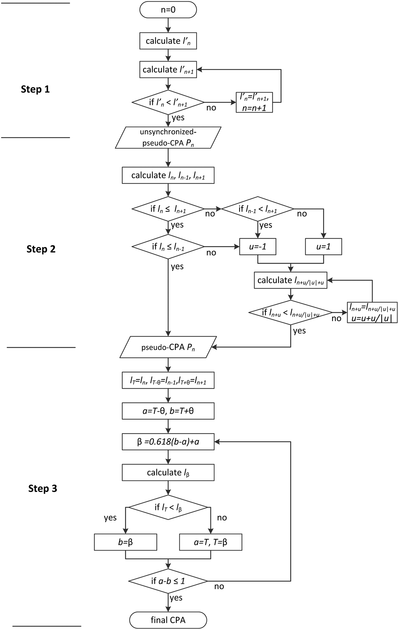
Figure 10. Process of calculating CPA.
4. CASE STUDIES
4.1. Application situations
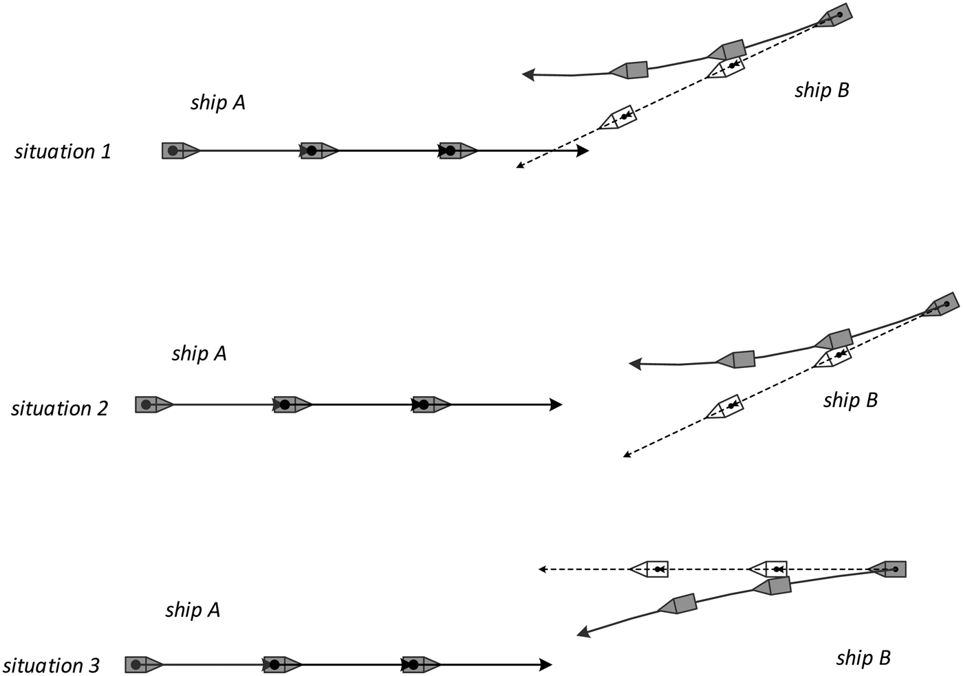
From the predicted positions, a more accurate CPA can be calculated by the proposed method to assist the shore operator in clarifying approaching situations. In Figure 11, three approaching scenarios are shown as examples. In Situations 1 and 2, ship A is the stand-on ship and ship B is the give-way ship (International Maritime Organization, 1972). The demonstrated method can help the shore operator give guidance to these two ships in order to make their rational decisions immediately and facilitate the collision avoidance process.

Figure 11. Some situations where the developed method is useful for safety assessments.
In Situation 1, a collision avoiding alteration has been made by ship B through changing course to starboard. Using the traditional method, the predicted trajectory of ship B (shown with the dotted line) is indicating a high probability of a collision. Although the bridge of ship A can observe the changing course of ship B, the officer may not be clear about whether a response should be taken to avoid a close-quarters situation and reduce the risk. Using the method developed in this paper, it is very clear that ship B has changed its route and will navigate safely when passing and ship A does not need any action.
In Situation 2, ship B is also the give-way ship. This shows that the vessels are not in direct risk of collision, but would pass much closer than normally considered prudent for ship B to pass in the front of ship A. According to COLREGs, these two ships would better pass by each other port side to port side, with an alteration of course to starboard by ship B. Again the danger is that the course change of ship B may not be observed clearly by ship A in a short time or in reduced visibility, and the officer of ship A may decrease the speed or change the course to reduce the collision risk once the close-quarters situation has formed. Using the developed method, it is very clear that ship B has changed the route and will pass on the port side of ship A safely. Only if the calculated DCPA is too short for safety does a simple starboard course change need to be taken to maintain safety.
In Situation 3, ship A and ship B are navigating with a reciprocal course and will pass each other on the port side. In this situation, it is very dangerous if something goes wrong with ship B, such that ship B is turning or drifting to port. The sooner this small change in ship track is observed by the officer of ship A, the better. The traditional method is very slow to detect the tiny change of the approaching situation. However, the proposed method can help shore operators identify this emergency situation quickly and reduce the risk of ships.
4.2. Real-life practical application
The developed method has been adopted by the Early Warning System of the Bridge Waterways in the Yangtze River to ensure the safety of the waterways near bridges. In this early warning system, all the obstacles, such as buoys, bridge piers and shoals, are deemed to be targets with SOG zero and COG zero like static ships. The alarm values of DCPA and TCPA can be set by supervisors according to their experience. The parameter α should be ascertained firstly according to the historical data. Through adjusting the value of α in the range [0, 1], the final α can be obtained when the minimum errors of the predicted positions are found. The obtained parameter α in the area of interest varies from upstream ships to downstream ships. According to minimum errors, the parameter α is 0·8 for upstream ships while it is 0·5 for downstream ships. In this case study, the maximum value of the distance between a prediction position and the corresponding position is usually less than 80 metres if the prediction period is three minutes.
In the Wuhan Bridge Waterway, a downstream ship named ‘Liyuan2’ whose home port was Chongqing Port was navigating to Jiujiang Port with a load of 5,100 tonnes of stones. At about 1100 am on 2 February 2014, the steering system of this ship broke down when passing by the No.1 buoy before proceeding through the Wuhan Yangtze River Bridge. This ship collided with and damaged the No.8 pier of the bridge because of the drift. It is worth noting that there is a strong current pushing downstream ships to the starboard side in this waterway. The ship course therefore should not be just perpendicular with the bridge but slightly to the port side to overcome the current, as shown in Figure 12. The Early Warning System was supervising the entire waterway using AIS data at that time. The monitoring interfaces are shown in Figures 12 and 13 which show the situation over 30 seconds using the proposed method.

Figure 12. Liyuan2's normal navigating monitor interface (at 11:20:43 am).

Figure 13. Liyuan2's anomalous navigating monitor interface (at 11:21:13 am).
In Figure 12, it is shown that the ship was navigating normally (the course is slightly to port in order to cope with the current) and would pass the bridge safely. Meanwhile, the white buoy (No.1 buoy) at the port side was considered as a static target, it alarmed that the DCPA between the ship and the buoy was too small. This buoy is marked by a red square by the system in Figure 12.
In Figure 13, it is shown that the system would show that this ship was drifting and deviating to the starboard side of the channel at 11:21:13 am. It especially would have shown that the ship was reducing its speed, which is actually not normal when crossing under the bridge. The ship position was anomalous and deviated to pass the bridge, while the ship might collide with the No.8 pier under the current drift. DCPAs between the ship and the two buoys were also too close. These two buoys are marked by red squares in the system.
The same situation using the traditional CPA method would alarm some 30 seconds later. Therefore by using the method developed in this paper, there would have been an earlier and timely warning to assist Vessel Traffic Services (VTS) and seafarers in detecting high risk navigational behaviours effectively in many cases.
5. CONCLUSIONS
CPA results by existing methods which only consider SOG and COG are imperfect and a CPA calculation method taking account of SOG, COG, COS and ROT is required. AIS can provide information on all four essential factors, as well as the position and other important information. AIS data is therefore suitable to predict the positions and calculate CPA. To obtain an accurate CPA, a ship position prediction model is firstly built to extract an accurate trajectory using AIS data. In addition, a CPA calculation method is developed to calculate the final CPA with the asynchronous AIS data.
A CPA obtained by the proposed method can assist the ship officer and VTS supervisor in clarifying the approaching situations, making the correct decision immediately, and simplifying the collision avoidance process. The proposed method has been adopted by the Early Warning System of Bridge Waterways on the Yangtze River. A real collision scenario is used to show that the CPA calculation method can assist in detecting high risk navigating behaviours effectively and in a timely manner.
This four-factor method has been developed for implementation in VTS shore facilities where only asynchronous data received from the ship AIS units is available. The principle of using the four factors (SOG, COG, COS and ROT) to predict CPA can be tailored to applications on ship bridges to improve CPA prediction when one or more ships are manoeuvring in close proximity.
The proposed method for CPA calculation may be more complicated than the conventional methods. Further work may be needed to extensively test the method and its applicability. It may also be useful to take into account more relevant factors in the real DCPA calculation although the complexity of the method would be increased.
ACKNOWLEDGEMENTS
Grateful acknowledgement is made to the Changjiang Maritime Safety Administration who provided us with considerable help when the proposed method was validated.
FINANCIAL SUPPORT
This paper was supported by the National Natural Science Foundation of China (Grant No. 51309187) and FP7 Marie Curie IRSES of European Union (Grant No.314836).