1. Introduction
Nowadays, the global positioning system (GPS), in a coded solution, is the primary method of position determination in modern air (Lachapelle et al., Reference Krasuski and Savchuk1996; Ochieng et al., Reference Naranjo, Jiménez, Aparicio and Zato2003; Brodin et al., Reference Brodin, Cooper, Walsh and Stevens2005; Krasuski et al., Reference Krasuski, Ciećko, Bakuła and Wierzbicki2020; Krasuski and Savchuk, Reference Krasuski, Ciećko, Bakuła and Wierzbicki2020), land (Ojeda and Borenstein, Reference Ochieng, Sauer, Walsh, Brodin, Griffin and Denney2007; MacLean, Reference Lachapelle, Cannon, Qiu and Varner2009; Naranjo et al., Reference Merry and Bettinger2009; Zandbergen and Barbeau, Reference van Diggelen2011; Sun et al., Reference Specht2017; Merry and Bettinger, Reference MacLean2019; Elhajj and Ochieng, Reference Elhajj and Ochieng2020; Robustelli et al., Reference Ramesh, Jyothi, Vedachalam, Ramadass and Atmanand2021) and marine (Grant et al., Reference Grant, Williams, Ward and Basker2009; Han et al., Reference Han, Park, Kim and Son2016; Ramesh et al., Reference Ojeda and Borenstein2016; Bhatti and Humphreys, Reference Bhatti and Humphreys2017; Glomsvoll and Bonenberg, Reference Glomsvoll and Bonenberg2017) navigation. Its use depends primarily on the positioning accuracy, which has been constantly changing over the last years, hence GPS applications depend on the current positioning accuracy of that system (Rudnicki and Specht, Reference Robustelli, Paziewski and Pugliano2016; Specht, Reference Specht2019). For this reason, it is important to determine the current GPS accuracy because it is decisive for the possibilities of using the system in various navigation applications.
The accuracy of navigation system positioning is determined by measurement (Specht, Reference Śniegocki, Specht and Specht2010, Reference Specht2010; Śniegocki et al., Reference Rudnicki and Specht2014). The results are processed using statistical methods, where the values of the mean squared errors (MSEs) sφ and sλ are calculated, according to the relationships (Hofmann-Wellenhof et al., Reference Hofmann-Wellenhof, Legat and Wieser2003):


where:
sφ is standard deviation of geographic latitude,
sλ is standard deviation of geographic longitude,
${\delta _{{\varphi _i}}}$
 is geographic latitude error for i-th measurement,
${\delta _{{\lambda _i}}}$
is geographic longitude error for i-th measurement,${\overline {{\delta _\varphi }} _n}$
is sample mean of geographic latitude errors,${\overline {{\delta _\lambda }} _n}$
is sample mean of geographic longitude errors,n is number of measurements.


Next, based on the calculated standard deviation values, the distance root mean square (DRMS) (probability of 63⋅2–68⋅3%) is determined as a basic measure for navigation system positioning accuracy. However, to ensure higher statistical reliability for assessment of the accuracy of the system, it is commonly accepted in navigation to use its double value, that is, twice the DRMS (2DRMS) (probability of 95⋅4–98⋅2%) depending on the ellipticity of the equal probability ellipses associated with the position error. This is described by the following relationship (Hofmann-Wellenhof et al., Reference Hofmann-Wellenhof, Legat and Wieser2003):

The 2DRMS measure is commonly used in navigation because it has advantages, including: straightforward method to analyse data, readily applied to the Monte Carlo method and highly compatible with a geometric dilution of precision (GDOP) analysis. The disadvantages include not being tied to a specific probability level and being skewed by large errors (Chin, Reference Chin1987).
In navigation positioning systems, it is assumed that φ and λ errors are normally distributed (Bowditch, Reference Bowditch1984; Cutler, Reference Cutler2003; Hofmann-Wellenhof et al., Reference Hofmann-Wellenhof, Legat and Wieser2003). This is dictated by many factors, the most important being the simplicity of calculations and the widespread use of Gauss statistics in science and technology. However, it should be noted that approximating φ and λ error distributions with a normal distribution results in a significant difference between two position accuracy measures in the horizontal plane (2D): 2DRMS and Radius 95% (R95). Figure 1 presents the histograms of GPS position errors defined with respect to φ and λ. The graphs come from the U.S. Department of Defense (U.S. DoD, Reference Sun, Odolinski, Xia, Foster, Falkmer and Lee1993). On this graph, comments have been drawn on the differences between the empirical distribution and the typical normal distribution for both variables. They clearly show that φ and λ error distributions exhibited a positive kurtosis (more centred concentration) in 1993 together with some asymmetry.
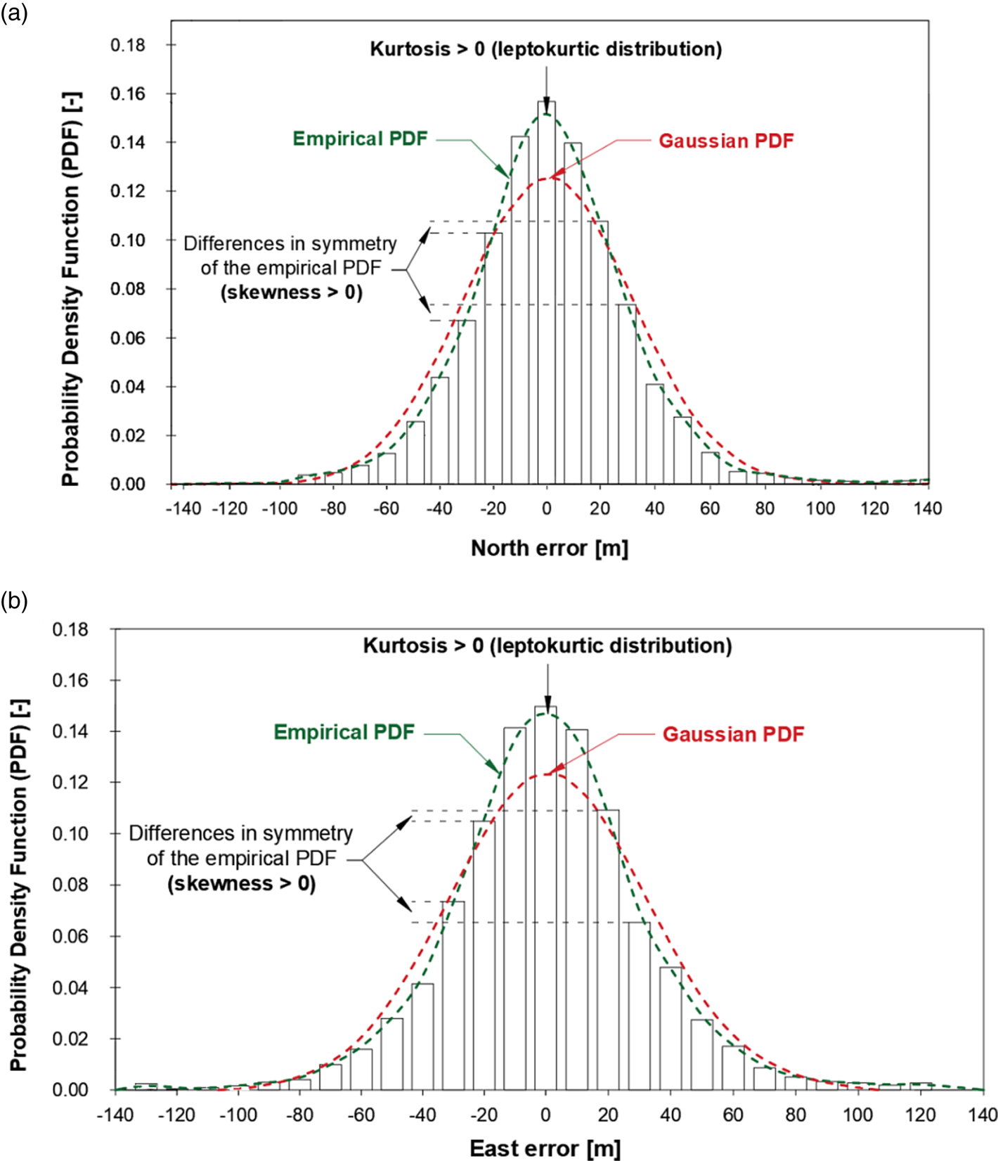
Figure 1. Distributions of GPS latitude (a) and longitude (b) errors (U.S. DoD, Reference Sun, Odolinski, Xia, Foster, Falkmer and Lee1993) together with comments on their selected statistical features influencing the lack of fit between empirical data and the normal distribution
What is visible in Figure 1 are the differences in fit between the empirical GPS data (δφ and δλ) and a typical normal distribution, which cause the difference between the 2DRMS and R95 values. In the case presented in Figure 1, the empirical value of R95 was 64 m, whereas the theoretical value, determined by calculating the 2DRMS measure, was 83 m. Both values differ by 29⋅69%.
Frank van Diggelen (1998) raised this issue by pointing out that distribution matches a true Gaussian distribution in each bin if the bins are 1 m wide (that is, the bins are 10% the width of the 4σ range of the distribution). Note that, in the 1998 paper, the same test was performed for differential GPS (DGPS) with similar results. The distribution matched a true Gaussian distribution with bins of about 10% of the 4σ range of errors – except that, for DGPS, the 4σ range was approximately 1 m, and the bins were 10 cm.
In Kalafus and Chin (Reference Kalafus and Chin1986) and Chin (Reference Chin1987) very detailed statistical analyses of GPS position errors were conducted. Their goal was to obtain the distribution of GPS position accuracy measures over the 24 h period. A total number of 2,178 cases were analysed (for 21 satellites). The east-west accuracy (2σ) was 45⋅8 m, while the north-south accuracy (2σ) was 61⋅5 m. Moreover, the 2DRMS value was 76⋅7 m and the R95 value was 66⋅5 m. Note that these results were obtained with selective availability enabled. This study has shown that the east-west accuracy of GPS is better than north-south accuracy. The difference between the 2DRMS and R95 values was 15⋅33%.
Statistical studies of global navigation satellite system (GNSS) position errors conducted on very large samples ranging from one million to more than two million fixes were analysed in Specht (Reference Śniegocki, Specht and Specht2010, Reference Specht2010) and Śniegocki et al. (Reference Rudnicki and Specht2014). All measurement campaigns were performed at coordinates: φ = 54°31⋅756087’ N, λ = 18°33⋅574138’ E (Gdynia, Poland) with a frequency of 1 Hz and the measurement data were recorded using the National Marine Electronics Association (NMEA) standard. This research confirmed that the position errors of DGPS and European Geostationary Navigation Overlay Service (EGNOS) systems are also different for φ and λ measurements, with latitude measurements exhibiting larger errors. Moreover, the differences in determination of 2DRMS against R95 values were:
• 13⋅97% during the DGPS 2006 measurement campaign (2,187,842 fixes) for which 2DRMS = 2⋅04 m and R95 = 1⋅79 m (Śniegocki et al., Reference Rudnicki and Specht2014).
• 15⋅66% during the DGPS 2014 measurement campaign (951,698 fixes) for which 2DRMS = 0⋅96 m and R95 = 0⋅83 m (Śniegocki et al., Reference Rudnicki and Specht2014).
• 15⋅74% during the EGNOS 2006 measurement campaign (1,774,705 fixes) for which 2DRMS = 8⋅82 m and R95 = 7⋅62 m (Specht, Reference Specht2010).
• 13⋅37% during the EGNOS 2010 measurement campaign (1,481,660 fixes) for which 2DRMS = 1⋅95 m and R95 = 1⋅72 m (Specht, Reference Śniegocki, Specht and Specht2010).
These differences are due to differences in sφ and sλ estimation and the position random walk, which occurred in both of the analysed systems, but was slower than in the GPS system (Specht, Reference Specht2021).
Note that in each of the considered cases, the actual accuracy value (R95) for DGPS and EGNOS systems was higher than the accuracy value calculated from the 2DRMS relation. This indicates that the empirical position errors in the determination of φ and λ by DGPS and EGNOS systems are more concentrated around the real value than the probability density function (PDF) calculated with the normality assumption. This corresponds to the conclusions on error concentration presented by the U.S. Department of Defense (U.S. DoD, Reference Sun, Odolinski, Xia, Foster, Falkmer and Lee1993) and van Diggelen (1993). It also confirms that 2DRMS values are overestimated relative to R95, as described in Kalafus and Chin (Reference Kalafus and Chin1986) and Chin (Reference Chin1987). Note, however, that the magnitude of this difference (for both 2DRMS and R95) is different for both DGPS and EGNOS systems.
Studies of the statistical features of DGPS and EGNOS position errors presented in Specht (Reference Specht2021) carried out on a very large series of fixes (900,000) have shown that, for both systems, errors are more concentrated around the mean value than in the case of normal distribution, which is evidenced by kurtosis different from zero, and the error distribution exhibits a small skewness, which is indicative of its slight asymmetry. Figure 2 presents an example of statistical distributions of φ errors by the DGPS system in 2006 and λ errors by the EGNOS system in 2014.

Figure 2. Statistical distributions of latitude errors by the DGPS system in 2006 (a) and longitude errors by the EGNOS system in 2014 (b)
For navigation positioning systems, such as GPS, the process of position determination exhibits a special feature called the position random walk (PRW) which consists of wandering of GPS position coordinates. This phenomenon results from both the iterative method used to determine coordinates and the use of Kalman filtering. It results in the following position being determined based on the previous one, which causes subsequent positions to appear closer to one another. Figure 3 presents the PRW phenomenon, where grey colour presents the distribution of 168,286 fixes determined by the GPS system in 2013 (typical code receiver) in relation to the average value. Sub-sessions consisting of 1,000 fixes each have been marked with different colours. On the right side, Figure 3 shows the change in mean coordinates determined for successive sub-sessions and the distance between them.
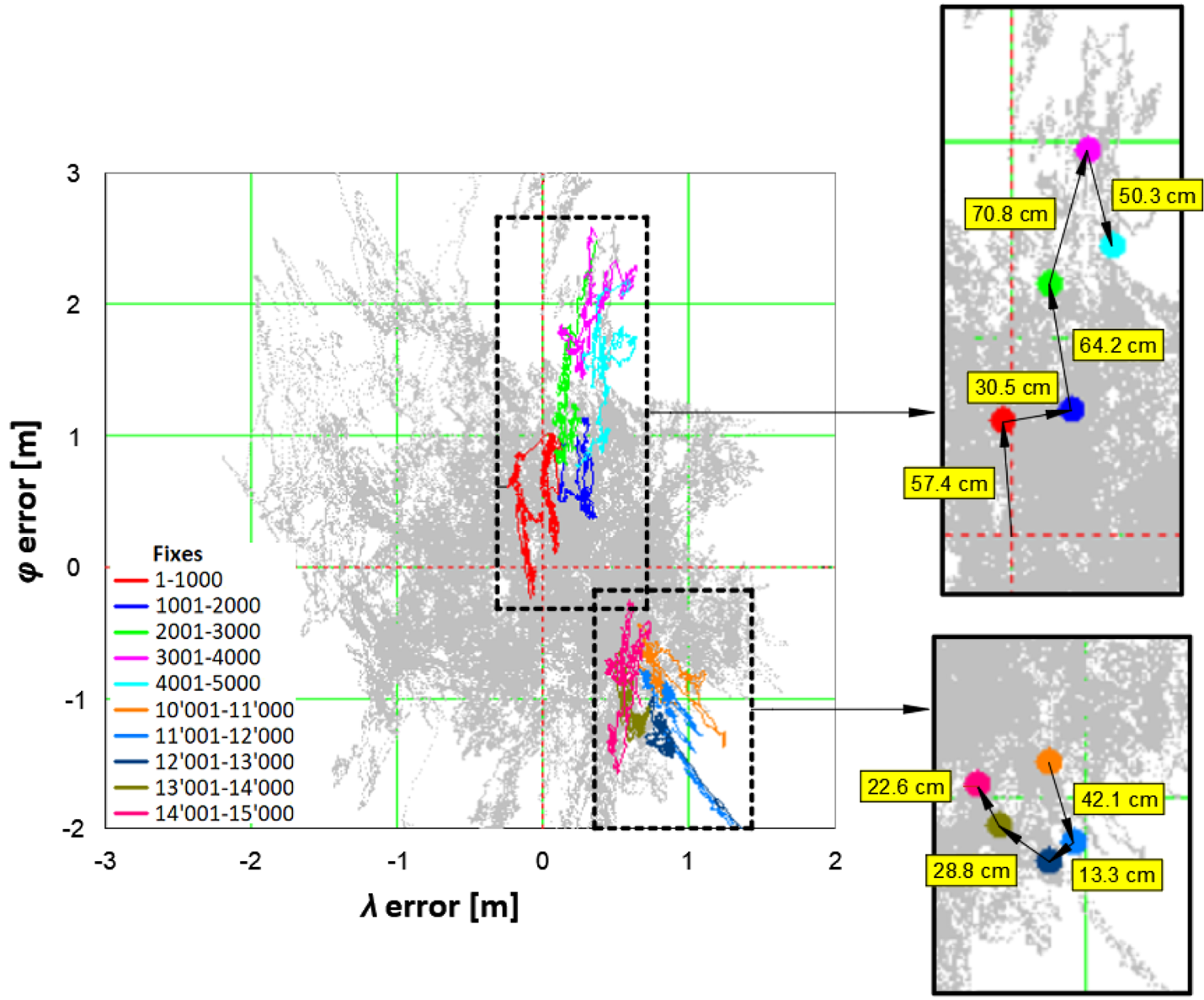
Figure 3. PRW phenomenon for the GPS system in 2013
The whole measurement campaign was divided into smaller sub-sessions consisting of 1,000 fixes. The red colour indicates the results of session 1 (measurements: 1–1,000), blue indicates the results of session 2 (measurements: 1,001–2,000), green indicates the results of session 3 (measurements: 2,001–3,000), purple indicates the results of session 4 (measurements: 3,001–4,000) and sky-blue indicates the results of session 5 (measurements: 4,001–5,000). To prove that the phenomenon is permanent, an identical analysis was performed for sub-session (1,000 fixes each) which included measurements numbered: 10,001–11,000, 11,001–12,000, 12,001–13,000, 13,001–14,000 and 14,001–15,000.
On the right side of Figure 3 are marked with dots mean coordinates (φ and λ) calculated based on 1,000 fixes in each sub-session. Moreover, to estimate at which speed the average coordinates move (from every 1,000 fixes), the distances between the mean coordinates were added to the figures. They show that the walking speed for average coordinates (from 1,000 consecutive fixes) can be estimated in the case under analysis at 13⋅3–70⋅8 cm per 1,000 s. Obviously, this is only an estimate determined as in Specht (Reference Specht2020).
Another very important conclusion from Figure 3 is that if only a few thousand measurements were used to assess the GPS accuracy from this session, the calculated statistics (2DRMS and R95) would be far different and unrepresentative. This means that to assess the accuracy of GPS, the length of the measurement session cannot be arbitrarily determined, as is commonly the case in contemporary literature on the subject. Therefore, a preliminary study was conducted to estimate roughly a representative sample of measurements for a specific navigation positioning system (Specht, Reference Specht2020). It showed that this quantity depends on the accuracy of the navigation system positioning. For the GPS system, it was observed that for a session performed in 2013, the 2DRMS value stabilised at around 78,000 fixes. For the DGPS system, the value was around 31,000 fixes. Undoubtedly, higher positioning accuracy results in a shorter sample, ensuring the representativeness of the measurement campaign.
This paper describes research undertaken to evaluate the analyses of the distributions of GPS position error statistics in one-dimensional (1D) and two-dimensional (2D) space. Moreover, statistical distribution measures were determined using statistical tests, the hypothesis on the normal distribution of φ and λ errors was verified, and the consistency of GPS position errors with commonly used statistical distributions was assessed together with finding the best fit.
The measurements reported in this paper involved four identical code receivers, two of which operated in GPS mode while the other two operated in multi-GNSS mode, that is, with GPS/GLObal NAvigation Satellite System (GLONASS). To ensure the representativeness of the study, each of them took one million fixes.
The research aims were:
1. Determination of statistical measures describing the distributions of φ and λ errors, as well as their characteristics.
2. Determining the fit between φ and λ errors (analysed separately) and the normal distribution of GPS measurements.
3. Determining differences between GPS accuracy values calculated using 2DRMS and R95.
4. Evaluation of other statistical distributions for better approximation of the distribution of GPS position errors in 1D and 2D space.
This is the fourth paper in a series of monothematic publications, ‘Research on empirical (actual) statistical distributions of navigation system position errors’. The main scientific aim of this series is to answer the question of what statistical distributions follow the position errors of navigation systems such as GPS, GLONASS, BeiDou Navigation Satellite System (BDS), Galileo, DGPS, EGNOS and others. It must be emphasised that the purpose of both this paper and the whole series of publications is not to analyse the causes of PRW, such as ionospheric and tropospheric effects, multipath, noise, etc. This paper rather analyses the statistical distributions of 1D and 2D position errors resulting from PRW. The causes might be very complex and probably deserve a separate series of publications.
2. Materials and methods
2.1 Statistical distribution measures
Studies of the distribution of position errors for such systems as Decca (1993), GPS (2013) (Specht, Reference Specht2020), DGPS (2006 and 2014) and EGNOS (2006 and 2014) (Specht, Reference Specht2021) made it possible to establish both the methodology for this type of analysis and useful dispersion measures of navigation positioning system errors. The following measures were adopted as the most important and those that allowed for statistical inference in analyses of GPS position errors:
• PDF of empirical position errors.
• Histogram of empirical position errors.
• Cumulative distribution function (CDF) of empirical position errors.
• Other statistical measures such as arithmetic mean, kurtosis, median, quantiles, range, skewness, standard deviation and variance.
The PDF of empirical position errors, which is the GPS position error, may be determined separately for φ and λ or jointly – as the 2D position error. In real measurements, it is a natural, very intuitive and often the most convenient description of the probability distribution by means of a function. The probability density provides a mathematical apparatus that can be conveniently used for theoretical considerations, practical calculations and illustration of measurement results. In line with the definition, the probability density is a measurable function $f:{{\mathbb R}^n} \to [{0,\infty } )$ such that:

for any event A (GPS position determination with a specified error).
This function makes it possible to determine the probability of any event (occurrence of a GPS position error with a certain value) and even multivariate statistical analysis of the system's position errors. The plot of the PDF can be interpreted very intuitively: the higher the value of this function at a given point, the higher the probability of the given random variable taking the value from the environment of that point (GPS position error).
In the analyses of statistical distributions of GPS position errors, a random variable will be considered T with the probability density f. The knowledge of probability density f allows for determining the probability of observing a random variable T (GPS position error) within a given time interval $[{{\tau_i},{\tau_j}} ]$ in line with the formula:

Let ${T_1},{T_2}, \ldots ,{T_n}$ be a sample taken from the distribution of GPS position errors with density f. The ways of estimating the density f from a sample ${T_1},{T_2}, \ldots ,{T_n}$
 will be analysed. For navigation positioning systems, the position determination process exhibits the special feature called PRW, hence it is very important here to ensure a representative number of measurements. Therefore, the analysis was conducted on a largely redundant number of observations of nearly one million fixes.
Since the issue analysed here consists of estimating a function, it raises problems related to the fact that the set of functions defined on ${\mathbb R}$ is incommensurably more numerous than the set ${\mathbb R}$
 . An unbiased estimator of the function f does not exist. Therefore, other quality criteria of the estimator will be analysed. Thus let ${\hat{f}_n}$
 be the estimator f obtained from the sample ${T_1},{T_2}, \ldots ,{T_n}$
 . The number $e({{{\hat{f}}_n}} )$
 given by the formula:

is the mean integrated squared error (MISE) of the estimator ${\hat{f}_n}$ . The value $e({{{\hat{f}}_n}} )$
 is the measure of the global average fit between the estimator ${\hat{f}_n}$
 and the estimated function f.
An example of using the PDF of empirical position errors is presented in Figure 4, which presents a histogram of empirical λ errors for the DGPS system (900,000 fixes from 2014) approximated using three PDFs derived from logistic, normal and Weibull distributions.
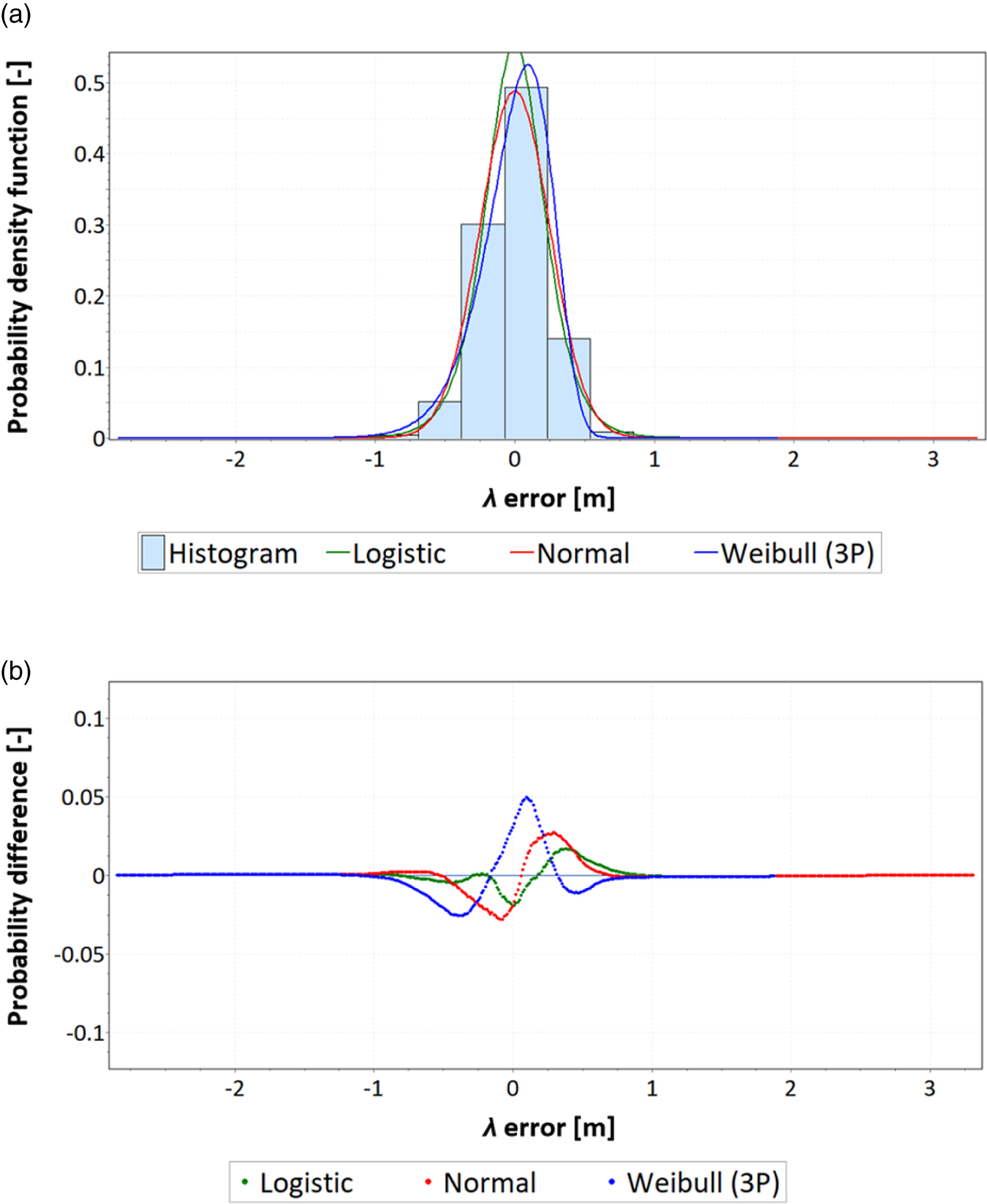
Figure 4. Distribution of empirical longitude errors for the DGPS system in 2014, their approximation using three probability density functions (a) and the differences between empirical data and theoretical distributions (b)
With the PDF of empirical position errors, it is possible to determine which of the statistical distributions is the best fit for the empirical data and for which fitting error values to the theoretical distributions are the smallest and largest. From Figure 4 it follows that logistic is the best-fitting distribution, whereas Weibull is the worst-fitting. In addition, it allows an analysis of selected statistical distribution measures: asymmetry (skewness), central tendency (arithmetic mean and median), concentration (kurtosis) and dispersion (range, standard deviation and variance).
The histogram of empirical position error is commonly used for processing and presenting data and it allows statistical inference. For this purpose, the whole interval of the sample in which the observed values of the random variable T (describing the position errors) fall has been divided into so-called ‘class intervals’ of equal length. All observations falling into a given class interval are represented by a single value from this class interval. The middle of the interval is the value representing a class interval. The sample elements represented by the individual centres of the class intervals should then be counted, which means that the size of individual class intervals should be determined.
In this way, a sequence of pairs of numbers $({{t_1},{n_1}} ), \ldots ,({{t_2},{n_2}} )$ is obtained, the first elements of which are the centre of the interval and the second elements of which are the size of this interval. Although the choice of class intervals is arbitrary, computational algorithms become much simpler when these are of equal length. The number of class intervals in a series depends on the variance in the characteristic under study (position error), the sample size and the purpose of the study. The number of intervals cannot be too small as this might blur important details of the sample and the regularity in the distribution of the variable. On the other hand, an excessively large number of intervals results in an excessive degree of detail that hinders the analysis and the drawing of conclusions about the distribution of the characteristic under analysis. There are no clear-cut rules for determining the number of classes r (position error intervals) for an n-element sample, but class width needs to be selected in such a way that the MISE (Equation [6]) is the smallest, irrespective of the estimated density. It can be assumed that the following inequality should be met:


and for very large values of n the minimum MSE is obtained for:


The constant c depends on the unknown density f through the intermediary of the value of ${\int {[{f(t )} ]} ^2}dt$ . This difficulty can be eliminated by choosing a constant c from a certain family of distributions. If, for example, f is the density of a normal distribution with variance σ 2, then the constant c is expressed by the formula:

By estimating σ from a sample ${T_1},{T_2},\ldots ,{T_n}$ , using the estimator:


we obtain a constant to be inserted into Equation (11). This method also provides good results for distributions other than normal.
The CDF of empirical position errors is a function determined based on frequency distribution calculated using the following formula:

The CDF ${\overline F _n}(t )$ is a step function, equal to zero for all t smaller than the smallest observed measurement and stepping by $1/n$
 for t equal to successive values of ti ($i = 1,2,\ldots ,r$
 ). The empirical CDF is an approximation of the true CDF from which comes the random sample (a series of GPS position error measurements). The determination of the empirical CDF function allows calculation of the differences between its values and the approximated values of theoretical CDFs of various statistical distributions. With empirical CDFs determined, it is possible to use the quantile–quantile (Q-Q) plot function in analyses. The use of this function allows a detailed analysis of the different dispersion measures depending on the random variable and the probabilities of its occurrence (empirical and theoretical). The Q-Q plot is a graph of the input (observed) data values plotted against the theoretical (fitted) distribution quantiles. Both axes of this graph are in units of the input data set. The Q-Q graphs are produced by plotting the observed data values δi ($i = 1,2,\ldots ,n$
 ) against the X-axis, and the following values against the Y-axis:

where:
F−1(δ) is the inverse CDF (ICDF) of geographic errors,
Fn(δ) is the empirical CDF of geographic errors,
δi is the geographic error for the i-th measurement.
The Q-Q plot will be approximately linear if the specified theoretical distribution is the correct model. EasyFit software displays the reference diagonal line along which the graph points should fall (Figure 5).
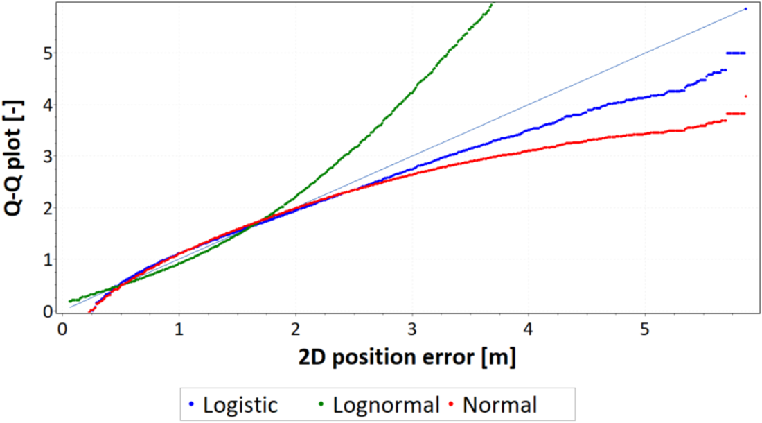
Figure 5. Example of the Q-Q plot of 2D position errors of a navigation system approximated by three statistical distributions
Other parameters, such as arithmetic mean, kurtosis, median, range, skewness, standard deviation and variance, as well as their use in analyses of statistical distributions of navigation positioning system errors, are described in detail in Specht (Reference Specht2021).
2.2 Description of GPS measurement campaigns
The research plan included two measurement sessions: the main session (900,000 fixes) and the verification session (237,000 fixes). Two typical (code) GPS receivers (Garmin GPS 19x HVS) were used in each series. Such receivers were chosen due to their popularity. The receivers worked in GPS mode only. The measurement was performed at coordinates: φ = 54°29⋅9740’ N, λ = 18°26⋅0947’ E (Gdynia, Poland) with a frequency of 1 Hz and the measurement data were recorded using the NMEA standard.
Simultaneous use of two receivers was intended to verify the repeatability of the results, whereas running two subsequent sessions (main and verification) allowed the representativeness of the statistics to be assessed. It was assumed that in the first session (main session) about one million fixes would be made by GPS 1 and GPS 2 receivers, whereas the next session (verification session) would cover about 0⋅25 million fixes. Research presented by Specht (Reference Specht2021) has shown that the length of the main session should ensure the representativeness of the results. Measurements for the first session were made from 8:30 p.m. on 22 February 2021 to 8:34 a.m. on 9 March 2021, giving 1,252,069 fixes. Measurements for the second series were made from 0:40 p.m. on 9 March 2021 to 6:31 a.m. on 12 March 2021 and yielded 237,084 fixes. The measurement results were verified for transmission errors using a checksum from the global positioning system fix data (GGA) message. For this purpose, copyrighted software was used, which deleted erroneous GGA messages. Since the measurements were conducted for two receivers located 1 m from each other, individual erroneous messages were deleted from both receivers in such a way as to obtain measurements performed in identical moments. For statistical analysis, data were prepared from the main session, which consisted of 900,000 fixes (for each of the two receivers), whereas for the verification session there were 237,000 fixes. The choice of 900,000 fixes resulted from the fact that similar analyses of position errors of DGPS and EGNOS systems (Specht, Reference Specht2021) were performed on exactly the same number of measurements. With the same session length, the results can be considered comparable. The coordinates of φ and λ were transformed (Gauss-Krüger transformation) to plane coordinates (x,y), expressed in metres, in line with mathematical relationships described in Deakin et al. (Reference Deakin, Hunter and Karney2010).
For position error calculations, algorithms were used developed in Mathcad software, additionally supplemented by EasyFit software. Measurement errors were compared with the mean values of φ and λ calculated from the whole population (repeatable accuracy).
3. Results
3.1 Analysis of 1D position errors
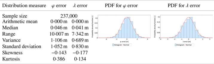
GPS position errors in 1D and 2D space necessitate separate statistical analyses – separate for φ and λ errors and separate for 2D position error. It was decided to present the results of 1D position error analyses (φ and λ) in a tabular form, unified for all sessions. The discussion will refer to two measurement sessions (main and verification), in which the results from measurements carried out by two GPS receivers (GPS 1 and GPS 2) are analysed. Tables 1 and 2 present the statistical distributions of φ and λ errors (separately) from two receivers (GPS 1 and GPS 2) obtained during the main session. The first column of those tables presents the statistical measures related to φ and λ variables, separately. These values were calculated based on empirical data (position errors). The second and third columns of Tables 1 and 2 present the histograms of φ and λ errors along with the PDFs, which were determined based on the minimisation of the MISE of the estimator.
Table 1. Statistical distributions and their measures determined for latitude and longitude errors (separately) for the GPS 1 receiver calculated based on measurements made during the main session
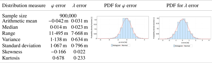
Table 2. Statistical distributions and their measures determined for latitude and longitude errors (separately) for the GPS 2 receiver calculated based on measurements made during the main session
Research showed that the beta, Student's, lognormal, normal and logistic statistical distributions best approximate φ errors (main session, GPS 1 receiver), whereas beta, normal, lognormal, gamma and logistic distributions best describe λ errors (main session, GPS 1 receiver).
At the same time, the fit between φ and λ errors was tested with the normal distribution (main session, GPS 1 receiver). For this purpose, the Kolmogorov–Smirnov test was used. The testing method has been described in detail by Specht (Reference Specht2020, Reference Specht2021). The test results gave no grounds to reject the hypothesis that φ and λ errors fit the normal distribution, for α = 0⋅05. On this basis, it was decided only to approximate the remaining histograms (main and verification sessions, GPS 2 receiver) using the PDF of the normal distribution.
The following conclusions can be drawn from the presented data from the main session:
• The results obtained and their statistics, made with two independently operating receivers, are very similar.
• The difference in arithmetic mean values is 8 mm for φ and 22 mm for λ.
• Significant differences between standard deviation values for φ (1⋅067 m and 1⋅117 m) and λ (0⋅796 m and 0⋅818 m) errors are worth noting. This means that the GPS system exhibits much larger errors in measuring latitude than longitude. This hypothesis is also confirmed by the range value, which is significantly larger for φ.
• For both coordinates, both sessions exhibit a small asymmetry (skewness), which is negative for φ and positive for λ. Skewness results combined with low arithmetic mean values indicate that, for both coordinates, the distributions of errors can be considered symmetric and the estimation of the arithmetic mean value exhibits a high accuracy. This is also confirmed by the result of testing the fit between φ and λ errors with the normal distribution.
• Both φ and λ errors exhibit leptokurtic characteristics (Kurt>0), which means that errors are more concentrated around the central value than in the normal distribution. In this context, it should be noted that the kurtosis value for φ errors is two to three times larger than for λ errors. This feature has also been observed in DGPS and EGNOS systems (Specht, Reference Specht2021).
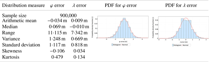
The presented conclusions from the main session were verified with measurements of the verification session, whose size was limited to 237,000 fixes. The verification session was intended to confirm the results obtained in the main session. Note that since the number of measurements in the verification session was three times smaller, slight differences in the estimation of particular measures should be considered acceptable. Tables 3 and 4 present the statistical analyses related to the verification session in a form identical to Tables 1 and 2.
Table 3. Statistical distributions and their measures determined for latitude and longitude errors (separately) for the GPS 1 receiver calculated based on measurements made during the verification session
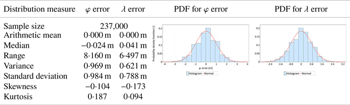
Table 4. Statistical distributions and their measures determined for latitude and longitude errors (separately) for the GPS 2 receiver calculated based on measurements made during the verification session

The following conclusions can be drawn from the verification session compared with the main session:
• Analyses of the mean value and standard deviation present results similar to the main session. The hypothesis that φ errors are larger than λ errors was confirmed.
• The positioning accuracies, defined by the standard deviation of both variables (φ and λ errors), were very similar in both sessions.
• Similar to the case of the main session, slight skewness (asymmetry) in the distributions of φ and λ errors was observed.
3.2 Analysis of 2D position errors
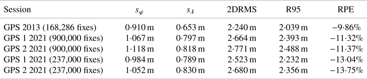
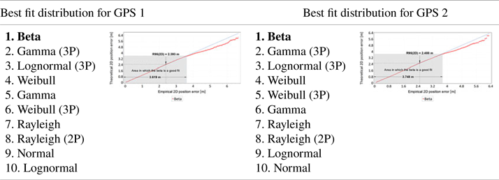
The differences found in the values of sφ and sλ should influence the GPS position error statistics, determined in the horizontal plane (2D). Tables 5 and 6 present the analyses of 2D position errors for both GPS receivers (main session). A histogram, PDFs of different statistical distributions and a Q-Q plot were used for the analyses. The first column of Table 5 shows the results of position error statistics related to the percentile statistics of 2D position errors for the GPS system. What is particularly important here is the value of the 95% statistic, as it is identical to the R95 measure commonly used in navigation. The second and third columns of Table 5 present the histograms of 2D position errors for two GPS receivers, approximated by the beta distribution. The use of beta distribution for approximation is justified by its very good fit with empirical distributions of GNSS systems such as DGPS and EGNOS (Specht, Reference Specht2021). Those statistical distributions (starting from the best one) that approximated 2D position errors for the GPS system most accurately are listed in the first column of Table 6. These have been supplemented with a Q-Q plot that shows the differences between the beta distribution and the empirical position errors. Moreover, the grey rectangle on the Q-Q plots indicates the area in which the beta statistical distribution is a good fit for GPS position errors.
Table 5. Statistical analysis of 2D position errors for two receivers (GPS 1 and GPS 2) in the main session
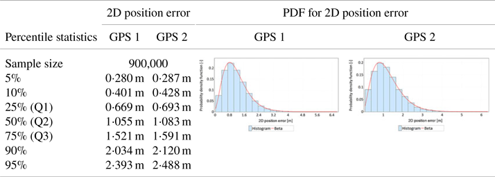
Table 6. Analysis of fit between empirical data of 2D position error and theoretical distributions for two receivers (GPS 1 and GPS 2) in the main session
An analysis identical to the main session was conducted for the verification session. The results of this session are presented in Tables 7 and 8. The structure of Tables 7 and 8 and the interpretation of the presented results are identical to Tables 5 and 6.
Table 7. Statistical analysis of 2D position errors for two receivers (GPS 1 and GPS 2) in the verification session
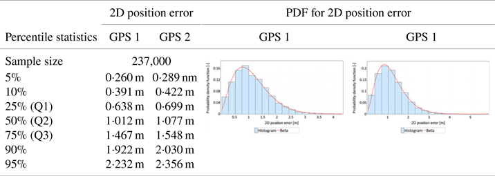
Table 8. Analysis of fit between empirical data of 2D position error and theoretical distributions for two receivers (GPS 1 and GPS 2) in the verification session

The following conclusions can be drawn from Tables 5–8:
• The values of the R95 measure in the main session were 2⋅393 m (GPS 1 receiver) and 2⋅488 m (GPS 2 receiver), respectively. Similar values, 2⋅232 m (GPS 1 receiver) and 2⋅356 m (GPS 2 receiver 2) were obtained in the verification session. The difference in results of the main session is 9⋅5 cm, which may be indicative of the representativeness of the main session fixes. The results of the verification session are slightly worse, which may be due to the session length.
• The measurements of both sessions showed that the beta distribution best represents the statistical nature of 2D position errors for the GPS system. Gamma, lognormal and Weibull distributions present equally good fits of empirical GPS position errors.
• Q-Q plot analyses indicate that the beta distribution does well in approximating 2D position errors for the GPS system to values well above the position error determined with 95% probability. In the main session, this distribution well describes GPS errors up to a value of about 3⋅7 m. In the much shorter verification session, this value was about 3⋅5 m. It should be added that the position error value of 3⋅7 m in the main session was determined with a probability of more than 99⋅7% (3σ). This proves that the beta distribution can accurately approximate empirical GPS position errors practically over the whole range of probabilities (from 0 to close to 1).
Furthermore, as already shown, in the main session φ errors are about 34–37% larger than λ errors, hence, the calculation of the 2DRMS value must be quite different from the R95 value. Table 9 presents results of the 2DRMS calculation based on sφ and sλ in line with Equation (3). The last column of Table 9 presents the percentage value of the difference between the 2DRMS and R95 measures (relative percent error, RPE) determined in accordance with the following formula:

Table 9. The differences between the 2DRMS and R95 measures

Measurements made in 2013, with a session length of 168,286 fixes, were also included in Table 9.
4. Discussion
Both sessions showed that the positions are more scattered relative to φ than relative to λ. The difference seems significant, since it was 33⋅88% (GPS 1 receiver) and 36⋅67% (GPS 2 receiver) for the main session and was 24⋅71% (GPS 1 receiver) and 26⋅75% (GPS 2 receiver) for the verification session. In this context, it is worth mentioning the results of similar analyses conducted on data from 2013, which covered 168,286 fixes. Analysis of the 2013 data, where φ errors were compared with λ errors, produced a similar result of 39⋅36%.
Moreover, analysis and research of their results indicate the following statistical conclusions for GPS position errors:
• From the analysis of three sessions of different lengths, it follows that φ errors are larger than λ errors by 25–39%.
• A longer measurement session allows for decreasing the value of kurtosis for GPS position errors (especially for φ).
• As the measurement session gets longer, the value of skewness for φ and λ errors decreases, which leads to the conclusion that the distribution of both errors can be considered symmetrical.
• Latitude errors exhibit two to three times higher kurtosis, meaning that they are more concentrated around the central value than are longitude errors of this system.
The statistical characteristics described by the analysed distributions of φ and λ errors must result in a distribution of 2D position errors that is different from circular. Therefore, the use of a measure determining circular error, such as 2DRMS, must result in a discrepancy with respect to the R95 measure. The analysis of the results of 2D position errors showed that the actual accuracy of the GPS system determined by the R95 measure is lower than the value calculated using the 2DRMS measure. This is obvious, as both values relate to slightly different probabilities. The results of the conducted analyses are consistent with the conclusions of van Diggelen (1993) indicating a 10% difference between the 2DRMS and R95 measures. The results presented in Table 9 indicate that this difference is about 10–14%. Note also that a similar difference between the 2DRMS and R95 measures was obtained when determining the position error of DGPS and EGNOS systems (Specht, Reference Śniegocki, Specht and Specht2010, Reference Specht2010; Śniegocki et al., Reference Rudnicki and Specht2014). In a study of very long measurement sessions, a difference of 13–16% was obtained.
Referring to analogous analyses from the end of the 20th century, it should be noted that in 1993 the difference between the 2DRMS and R95 measures was 29⋅69% (U.S. DoD, Reference Sun, Odolinski, Xia, Foster, Falkmer and Lee1993), while research presented in the 1980s indicated that the difference between these measures was 15⋅33% (Kalafus and Chin, Reference Kalafus and Chin1986; Chin, Reference Chin1987). However, it should also be noted that these studies were carried out when the GPS system was operating with selective availability enabled.
5. Conclusions
Knowledge of the actual positioning accuracy of any navigation system, including GPS, is essential to correctly determine the applications in which the system can be used. In this paper, based on two measurement sessions (900,000 and 237,000 fixes), the distributions of GPS position error statistics in both 1D and 2D space have been analysed. Statistical distribution measures were determined using statistical tests, the hypothesis on the normal distribution of φ and λ errors was verified, and the consistency of GPS position errors with commonly used statistical distributions was assessed together with finding the best fit.
Research has shown that φ and λ errors for the GPS system are normally distributed. It was proven that φ and λ errors are more concentrated around the central value than in a typical normal distribution (positive kurtosis) with a low value of asymmetry. Moreover, φ errors are clearly more concentrated than λ errors. This results in larger standard deviation values for φ errors than λ errors. The differences in both values were 25–39%. Regarding the 2D position error, it should be noted that the value of 2DRMS is about 10–14% greater than the value of R95. In addition, studies show that statistical distributions such as beta, gamma, lognormal and Weibull are the best fit for 2D position errors in the GPS system.