


1. INTRODUCTION
In June 2017, during its 98th session (MSC98), the Maritime Safety Committee (MSC) of the International Maritime Organization (IMO) (2017) approved a new work plan for Maritime Autonomous Surface Ships (MASS). In recent years, MASS has become a popular research topic.
A key problem in researching MASS is planning a safe path at sea, in which automatic Collision Avoidance (CA) of all moving and stationary obstacles (for example, other ships, shallow waters, reefs, etc) is of vital importance. The complexities of CA for MASS lie in the following aspects: necessity to comply with the International Regulations for Preventing Collisions at Sea (COLREGS) (IMO, 1972), complex situations with multiple vessels, the existence of uncoordinated or uncertain CA actions for other Target Ships (TSs), and the real-time CA decision making of the Own Ship (OS) affected by a changing environment.
Early studies mainly addressed path planning or CA without considering COLREGS. Some examples include an extension of an Evolutionary Planner/Navigator (EP/N) named θ EP/N ++ that computes a safe and optimum path of a ship in given static and dynamic environments (Smierzchalski and Michalewicz, Reference Smierzchalski and Michalewicz2000); a Line of Sight Counteraction Navigation (LOSCAN) algorithm for CA in a two-ship encounter (Wilson et al., Reference Wilson, Harris and Hong2003); and a genetic algorithm to compute a safe navigation path in an open sea (Zeng, Reference Zeng2003). These methods are inherently unavailable for application in human-present ocean-going CA applications where COLREGS prevail.
Many path planning techniques with consideration of COLREGS have been developed in recent years, such as Artificial Potential Fields (APF) (Lee et al., Reference Lee, Kwon and Joh2004; Xue et al., Reference Xue, Clelland, Lee and Han2011; Lyu and Yin, Reference Lyu and Yin2017), a Velocity Obstacle (VO) (Kuwata et al., Reference Kuwata, Wolf, Zarzhitsky and Huntsberger2014), a Trajectory-Based Algorithm (TBA) (Lazarowska, Reference Lazarowska2017), the Ant Colony Optimisation (ACO) method (Lazarowska, Reference Lazarowska2015), Evolutionary Algorithms (EA) (Tam and Bucknall, Reference Tam and Bucknall2010), Fuzzy Logic (FL) (Brcko and Svetak, Reference Brcko and Svetak2013), and neural networks and hybrid intelligent systems (Perera et al., Reference Perera, Carvalho and Soares2012). However, some studies claim to be “COLREGS compliant” while allowing explicit violations of the rules in certain scenarios, such as making frequent and minor course alterations that are difficult to detect by other ships (Tam and Bucknall, Reference Tam and Bucknall2010) or turning to port when a collision risk exists (Perera et al., Reference Perera, Carvalho and Soares2012; Shah et al., Reference Shah, Svec, Bertaska and Klinger2014) even in a head-on situation (Tam and Bucknall, Reference Tam and Bucknall2010). Furthermore, some studies assume that all TSs maintain their course and speed (Lee et al., Reference Lee, Kwon and Joh2004; Perera et al., Reference Perera, Carvalho and Soares2012; Lazarowska, Reference Lazarowska2015; Szlapczynski, Reference Szlapczynski2015; Lazarowska, Reference Lazarowska2017; Lyu and Yin, Reference Lyu and Yin2017) or take COLREGS-compliant manoeuvres (Tam and Bucknall, Reference Tam and Bucknall2010) during problem solving. Once TSs perform changes of speed and/or course, even with a non-protocol action, the original solution based on these algorithms might be invalid. Again, some of them only simulated a single ship-to-ship encounter situation (Lee et al., Reference Lee, Kwon and Joh2004; Brcko and Svetak, Reference Brcko and Svetak2013; Szlapczynski, Reference Szlapczynski2015).
A Cooperative Path Planning (CPP) algorithm is a new contribution to path planning for MASS in multi-contact encounters. The main idea of this method is to compute a collision-free path for all ships involved (Xue et al., Reference Xue, Clelland, Lee and Han2011; Szlapczynski, Reference Szlapczynski2011; Tam and Bucknall, Reference Tam and Bucknall2013). This method supposes that all ships comply with COLREGS. Therefore, CA actions of these ships are predictable. In fact, encountered ships at sea may include both unmanned ships and human-operated ships, while non-COLREGS manoeuvres may exist and be hard to predict. Adopting a CPP strategy for all encountered ships relies on a means of wireless communication or coordination between them, such as the Automatic Identification System (AIS) (Woerner and Novitzky, Reference Woerner and Novitzky2017), Vessel Traffic Services (VTS) (Szlapczynski, Reference Szlapczynski2011) or a future more advanced technique.
In addition, for planning the path approaches of ships, one noticeable limitation is the computational time (at least a few seconds, for example, the CPP method and TBA, but over 200 s for an EA-based approach), which is significantly increased with the number of obstacles, making it difficult to achieve real-time navigation. One outstanding method based on simplified Model Predictive Control (MPC) can be used to manage complex scenarios with multiple dynamic obstacles with random motion (Johansen et al., Reference Johansen, Perez and Cristofaro2016). Unfortunately, this method does not consider static obstacles and might lead to higher time consumption. However, an expected feasible path for the OS considering real navigational constraints needs to be updated immediately due to the highly dynamic obstacles and environmental disturbances.
The APF method in particular (Lee et al., Reference Lee, Kwon and Joh2004; Xue et al., Reference Xue, Clelland, Lee and Han2011) has the ability to handle static and/or moving obstacles and considers some key rules from the COLREGS. Additionally, an artificial repulsive potential was included in a Non-linear Model Predictive Control (NMPC) method for controlling multiple Unmanned Surface Vehicles (USVs) in arbitrary formations (Fahimi, Reference Fahimi2007). However, this is a non-COLREGS potential field and only used for static obstacle avoidance.
Lee's method is capable of guiding a marine vehicle away from danger and returning to the pre-determined path by combining two heading angles in ‘track-keeping’ mode and ‘collision avoidance’ mode. However, the system incorporates over 200 fuzzy rules to determine the heading angle, which presents a challenge in computation time. Additionally, course alteration is fixed to a right-hand turn regardless of the obstacle's mobility, and only ship-to-ship encounter situations are presented in Lee's paper.
Xue's algorithm can address a complicated multi-ship encounter situation in the presence of some static obstacles. However, local minima limitations do exist in this method. The OS is obstructed by the obstacle and cannot reach the destination when the OS, the destination, and the obstacle lie on the same line with the obstacle in the middle. Additionally, this method assumes that all TSs exhibit COLREGS-compliant behaviour. No emergency scenarios or unforeseen circumstances are considered.
Table 1 shows a comparison of some typical approaches mentioned above in chronological order. These methods were evaluated according to the fulfilment of nine requirements/features: COLREGS compliance (a degree of fulfilment is specified as no, low, medium, or high), consideration of static and dynamic obstacles (quantities and shapes), motion features of the TSs (change of speed or/and course), consideration of dynamic properties, speed change in CA actions, and emergency CA actions for the OS, as well as computational time and repeatability of a solution. Some requirements are evaluated based upon fulfilment (yes in the table) or failure of fulfilment (no in the table) of a defined criterion. The computational time has its own scale of evaluation, where the time can be very low (milliseconds), low (seconds), medium (several or tens of seconds) or high (hundreds of seconds). In the last column this paper's method is evaluated for comparison with existing approaches.
Table 1. Comparison between different selected path planning and CA methods and the author's method for ships.

Notes: symbol “?” means that this subject is not specified or presented clearly in corresponding papers, “med” is the abbreviation of “medium”;
➀ the magnitude in the course change is standardised to one value of 30°;
➁ the running time is approximately linear with respect to the number of obstacles;
➂ a predictable change of speed or/and course as required by the COLREGS;
➃ dynamic properties of an OS are taken into account by considering the time needed for a ship to execute the calculated manoeuvre – course change;
➄ the turning manoeuvre directly affects the speed of the OS, not the speed change for CA action.
The rest of the paper is organised as follows: Section 2 describes the real-time path planning problem to be studied, including some assumptions, environment representations and requirements under COLREGS. Section 3 presents the path planning strategy based on a modified APF. Section 4 includes a model of the ship's motion. In Section 5, the results of the simulation are given. The last section summarises the achievements and limitations.
2. PATH PLANNING PROBLEM
This paper is concerned with the process of path planning for power-driven vessels in a complex environment modelled by static constraints and dynamic TSs.
2.1. Environment
The environment data can be collected by navigational aids such as a shipborne AIS, radar and Differential Global Positioning System (DGPS). Additional information can be provided from an Electronic Chart Display and Information System (ECDIS). The data input should include information about static obstacles and the real-time position, speed, and course of moving obstacles (TSs).
The collision shapes of static obstacles are simplified as circles and modelled as TSs with zero speed. This is not as precise as considering irregular shapes (Smierzchalski and Michalewicz, Reference Smierzchalski and Michalewicz2000). However, the circle collision shapes are simple and easy to expand into other shapes. For example, Xue et al. (Reference Xue, Clelland, Lee and Han2011) constructed coastlines and polygon land using discrete obstacle points, such as circle shapes, and convex and concave polygons in Lazarowska (Reference Lazarowska2017) are replaceable by the corresponding outer circles of these polygons. Additionally, the collision shapes of moving TSs are approximated as circles, as adopted in some recent studies (Tam and Bucknall, Reference Tam and Bucknall2013; Johansen et al., Reference Johansen, Perez and Cristofaro2016). Other domain shapes, such as hexagons and ellipses, which are used in Lazarowska's (Reference Lazarowska2017) CA algorithm by avoiding intersections with the boundaries of these shapes, are not suitable for use in the APF method at the moment.
2.2. Requirements
The path planning for ships has to fulfil some key requirements as follows:
• ability to avoid all the moving and stationary obstacles,
• COLREGS-compliant behaviours and the practice of good seamanship,
• nearly real-time operation for CA or path planning online,
• consideration of course changes for TSs, even with their uncoordinated behaviours,
• consideration of dynamic properties of the OS in a solved solution.
As compliance with COLREGS encompasses many different aspects, the focus in this study is about general vessel encounters, including conduct of vessels in sight of one another and operating under rules 13–17 for power-driven vessels. Categories of scope for COLREGS can be found in Woerner et al. (Reference Woerner, Benjamin, Novitzky and Leonard2016) and Woerner (Reference Woerner2016). Here, three primary encounter situations are considered: crossing, head-on, and overtaking. It is also worth considering Rule 8, which addresses general collision avoidance.
The CA action of the two ships potentially involved in a collision is defined as shown in Table 2, with the corresponding five regions illustrated in Figure 1. These regions are divided according to the relative bearings of TSs, such as 5°, 112·5°, etc. It should be specified that a head-on situation is somewhat vaguely defined by Rule 14 as “… meeting on reciprocal or nearly reciprocal courses…”, so 5° of the OS/TS heading line on either side is configured by the author for a tolerance of head-on, although it is not specified in the COLREGS. As required by Rule 8, the give-way vessel shall, as far as possible, take early and substantial action to keep well clear.
Figure 1. An illustration of the encounter situations.
Table 2. Encounters and Actions for OS and TSs

Many open-ocean scenarios involve speed changes (sometimes exclusively). This includes merchant ships slowing to a near stop rather than deviating course. However, such actions only occur when appropriate preventive action is not taken in good time. Under normal circumstances, mariners prefer to change heading rather than speed to avoid a collision. Therefore, course change is assumed as the primary strategy adopted for avoiding a collision in this article, which is suitable for the manoeuvres of the OS and all TSs.
In previous studies, the path planning solution is fixed and determined in advance based on ideal assumptions, such as all TSs maintaining their course and speed, or acting under the COLREGS. However, in reality, TSs may take unexpected actions. Even as the stand-on vessel, the OS has to take actions to avoid a collision due to absence or negligence of actions from a give-way TS at a short range. The reactive avoidance routine of the OS in an emergency collision situation should be considered to ensure safety (Campbell et al., Reference Campbell, Naeem and Irwin2012). This is one major aspect of concern in this study that differs from previous works.
3. THE PROPOSED STRATEGY
3.1. Collision risk assessment
The collision risk is assessed by two factors:
• Checking Criterion of Collision Risk (CC), which is used to determine if there is a collision risk with any TS when the current course for the OS is maintained;
• Checking Range of Collision Risk (CR), which is the distance the OS begins to scrutinise the risk of collision (Xue et al., Reference Xue, Clelland, Lee and Han2011).
The position and velocity of the OS and TS at one time step are denoted by p os, v os, p ts and v ts, respectively (see Figure 2). The safe boundary of the TS is expanded according to the domain radius of the OS and TS (that is, R os and R ts, respectively) and the allowable safe distance (d safe) is determined by the sea room, position sensor errors, and relative speed of the OS and TS in one time step. Therefore, the expanded circle's radius can be written as:
Figure 2. The vectors and CA strategy for ship-to-ship encounters.
 $$d_{m}=R_{os}+d_{safe}+R_{ts} $$
 $$\hbox{CR}=d_{m}+\rho_{o} $$
where ρ o is the influence range of the TS set by operators and is larger under conditions of low visibility, open waters, etc. The algorithm ignores obstacles outside the circle with a radius of CR. A large CR means an early CA action for the OS.
Additionally, in Figure 2, two tangent lines are drawn from the point p os to the expanded circle with a radius of d m. θ m is defined as the angle between any tangent line and the relative position vector p ot (i.e., p ts − p os), as in Equation (3).
 $$\theta_{{\rm m}}=\arctan\left(\displaystyle{{d_{m}}\over{\sqrt{\rho^{2}\lpar p_{os}\comma \; p_{ts}\rpar -d_{m}^{2}}}}\right)$$
θ is the angle between p ot and the relative speed vector v to (that is, v os − v ts). A risk of collision therefore exists when the extension line of v to crosses the circle with radius d m around the TS. Therefore, the CC can be written as follows:
 $$\theta \lt \theta_{\rm m} $$
3.2. Decision making with a modified APF
Original path planning to the goal is achieved through an attractive potential field. The attractive potential U att(p) is defined as a function of the relative distance between the OS and the goal:
 $$U_{att}\lpar p\rpar =\displaystyle{{1}\over{2}}\varepsilon\rho^{2}\lpar p_{os}\comma \; p_{g}\rpar $$
where ε is a positive scaling factor, and ρ(p os, p g) is the range between the OS and the goal.
The virtual attractive force is defined as the negative gradient of the attractive potential in terms of position:
 $$F_{att}\lpar p\rpar =-\nabla\lsqb U_{\rm att}\lpar p\rpar \rsqb =\varepsilon p\lpar p_{05}\comma \; p_{g}\rpar \overrightarrow{n_{og}} $$
where  $\overrightarrow{n_{og}}$ is a unit vector pointing to the goal position from the OS position.
If no risk is detected by the collision risk assessment module, the OS would proceed to the goal under the virtual attractive force. Otherwise, the CA manoeuvre subroutine is activated and computed through the repulsive potential field. Here, four subdivided zones around the OS (see Figure 3) are defined to determine the corresponding virtual repulsive potential. The distances between the OS and any TSs are indicated by d = ρ(p os, p ts). The τ is a small radius of an artificial safety margin of the OS, which guarantees that at the surface of the obstacles, the repulsive potential is sufficiently large but bounded (Ge and Cui, Reference Ge and Cui2002).
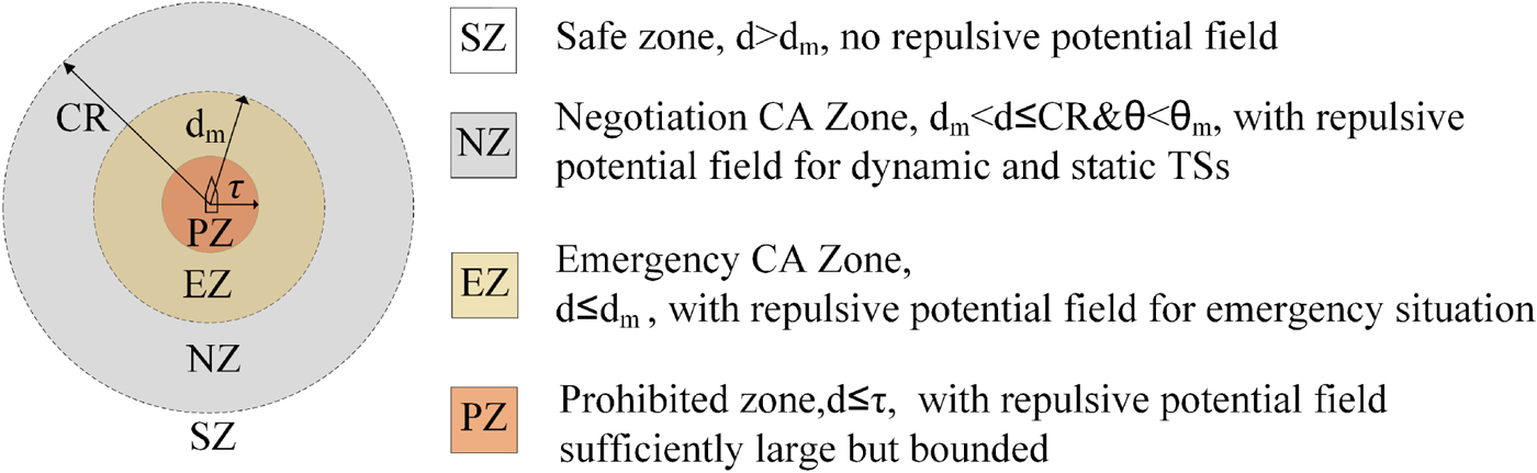
Figure 3. Subdivided zones around the OS.
Based upon the above, a new subdivided repulsive potential field function is proposed, which considers the CA for stationary and moving TSs giving sufficient sea-room, and the emergency CA at close range. It is noted that there are some zones where the resultant repulsive potential field is weakened or zero, even in the vicinity of an obstacle for the traditional APF model. A close-range emergency repulsion potential field function is included, which can produce a larger repulsion potential field than usual so that the OS could take an appropriate course alteration action immediately to keep well clear of all TSs. In addition to the conditions of no collision risk, sometimes the repulsive potential is also not defined, since there is no feasible solution for avoiding a collision with TSs in the case where TSs intentionally move towards the OS. Finally, the modified repulsion potential function is shown in Equation (7):
 $$\eqalign{ & U_{rep}\lpar p\comma \; v\rpar \hfill \cr & \quad =\left\{\matrix{\eta_{\rm d}R_{ts}\lpar e^{\theta_{m}-\theta}-1\rpar \left(\displaystyle{{1}\over{d-d_{m}}}-\displaystyle{{1}\over{\rho_o}}\right)^2d^2_g\comma \; \hfill & if\, v_{ts}\, {\ne}\, 0\comma \; \hbox{d}_{\rm m} \lt d \le \hbox{CR}\hbox{and }\theta \lt \theta_m \hfill \cr \displaystyle{{1}\over{2}}\eta_sR_{ts}\left(\displaystyle{{1}\over{d-\tau}}-\displaystyle{{1}\over{\rho_o}}\right)^2d^2_g\comma \; \hfill & if \, v_{ts}\, = \, 0\comma \; \hbox{d}_{\rm m} \lt d \le \hbox{CR}\, \hbox{and}\, \theta \lt \theta_m \hfill \cr \eta_eR_{ts}\left[\left(\displaystyle{{1}\over{d-\tau}}-\displaystyle{{1}\over{\rho^2}}\right)^2+\lpar \Vert V_{to}\Vert \cos \theta\rpar^2\right]d^2_g\comma \; \hfill & if\, d \le d_m \hfill \cr \hbox{not defined}\comma \; \hfill & \hbox{others}\hfill }\right.} $$
where η d and η s are the positive scaling factors for the dynamic TSs and static obstacles, respectively, at long distance, η e is the positive scaling factor for emergency CA action for the close-range obstacles, and d g = ρ(p os, p g).
The new corresponding repulsive force is defined as the negative gradient of the repulsive potential in terms of the positions and velocities:
 $$\eqalign{ F_{rep}\lpar p\comma \; v\rpar & =-\nabla U_{\rm rep}\lpar p\comma \; v\rpar \cr &=-\nabla_{p}U_{\rm rep}\lpar p\comma \; v\rpar -\nabla_{v}U_{\rm rep}\lpar p\comma \; v\rpar \cr & = \left\{\matrix{F_{rd1}+F_{rd2}+F_{rd3}\comma \; \hfill & if \, v_{ts}\, {\ne}\, 0\comma \; \hbox{d}_{\rm m} \lt d\leq \hbox{CR}\, \hbox{and}\, \theta \lt \theta_{{\rm m}} \hfill \cr F_{rs1}+F_{rs3}\comma \; \hfill & if\, v_{ts}=0\comma \; \hbox{d}_{{\rm m}} \lt d\leq \hbox{CR}\, \hbox{and}\, \theta \lt \theta_{{\rm m}} \hfill \cr F_{re1}+F_{re2}+F_{re3}\comma \; \hfill & if \, d\leq d_{m} \hfill \cr \hbox{not defined}\comma \; \hfill & \hbox{others}\hfill }\right.} $$
where:
 $$F_{rd1}=-\eta_{d}R_{ts}d_{g}^{2}\left[\left(\displaystyle{{1}\over{d-d_{m}}}-\displaystyle{{1}\over{\rho_{0}}}\right)e^{\theta_{{\rm m}}-\theta}\left(\displaystyle{{d_{m}}\over{d\sqrt{d^{2}-d_{m}^{2}}}}+\displaystyle{{\sin\theta}\over{\Vert v_{to}\Vert}}\right)+\displaystyle{{e^{\theta_{{\rm m}}-\theta}-1}\over{\lpar d-d_{m}\rpar^{2}}-F_{to0}}\right]\overrightarrow{n_{ot}} $$
 $$F_{to0}=\left(\displaystyle{{1}\over{d-d_{m}}}-\displaystyle{{1}\over{\rho_{0}}}\right)\left(\displaystyle{{d_{m}}\over{d\sqrt{d^{2}-d_{m}^{2}}}} +\displaystyle{{\sin\theta_{{\rm m}}}\over{\Vert v_{to}\Vert}}\right)$$
 $$\eqalign{F_{rd2} & = \pm\eta_{d}R_{ts}d_{g}^{2} \cr & \quad \left[\left(\displaystyle{{1}\over{d-d_{m}}}-\displaystyle{{1}\over{\rho_{0}}}\right)e^{\theta_{\rm m}-\theta}\left(\displaystyle{{1}\over{\Vert p_{ot}\Vert}}+\displaystyle{{\cos\theta}\over{\Vert v_{to}\Vert}}\right)+\displaystyle{{\Vert v_{ot\perp}\Vert\lpar e^{\theta_{{\rm m}}-\theta}-1\rpar }\over{d\lpar d-d_{m}\rpar^{2}}}-F_{to\perp}\right]\overrightarrow{n_{ot\perp}}} $$
 $$F_{to\perp}=\left(\displaystyle{{1}\over{d-d_{m}}}-\displaystyle{{1}\over{\rho_{0}}}\right)\left(\displaystyle{{1}\over{\Vert p_{ot}\Vert}}+\displaystyle{{\cos\theta_{{\rm m}}}\over{\Vert v_{to}\Vert}}\right)$$
 $$F_{rd3}=\eta_{d}R_{ts}d_{{\rm g}}\left(\displaystyle{{1}\over{d-d_{m}}}-\displaystyle{{1}\over{\rho_{0}}}\right)\lpar e^{\theta_{{\rm m}}-\theta}-1\rpar \overrightarrow{n_{og}} $$
 $$F_{rs1}=-\eta_{{\rm s}}R_{ts}\left(\displaystyle{{1}\over{d-\tau}}-\displaystyle{{1}\over{\rho_{0}}}\right)\left(\displaystyle{{d_{{\rm g}}^{2}}\over{d^{2}}}\right)\overrightarrow{n_{ot}} $$
 $$F_{rs3}=\eta_{{\rm s}}R_{ts}d_{{\rm g}}\left(\displaystyle{{1}\over{d-\tau}}-\displaystyle{{1}\over{\rho_{0}}}\right)^{2}\overrightarrow{n_{og}} $$
 $$F_{re1}=-2\eta_{{\rm e}}R_{ts}\left(\displaystyle{{1}\over{d-\tau}}-\displaystyle{{1}\over{d_{m}}}\right)\displaystyle{{d_{{\rm g}}^{2}}\over{\lpar d-\tau\rpar ^{2}}}\overrightarrow{n_{ot}} $$
 $$F_{re2}=2\eta_{{\rm e}}R_{ts}\displaystyle{{d_{{\rm g}}}\over{d}}\Vert V_{to}\Vert^{2}\lpar \cos\theta\sin\theta\rpar \overrightarrow{n_{ot\perp}} $$
 $$F_{re3}=2 \eta_{{\rm e}}R_{ts}d_{{\rm g}}\left[\left(\displaystyle{{1}\over{d-\tau}}-\displaystyle{{1}\over{d_{m}}}\right)^{2}+\Vert V_{to}\Vert^{2}\cos^{2}\theta\right]\overrightarrow{n_{og}} $$
In the NZ, the repulsive force determines that the passing side is to port or starboard for static obstacles yet only to starboard for dynamic TSs in order to meet the requirements of COLREGS. Figure 4 shows an illustration of a new repulsive force for a dynamic TS, so the total repulsive force F rd drives the OS to starboard.
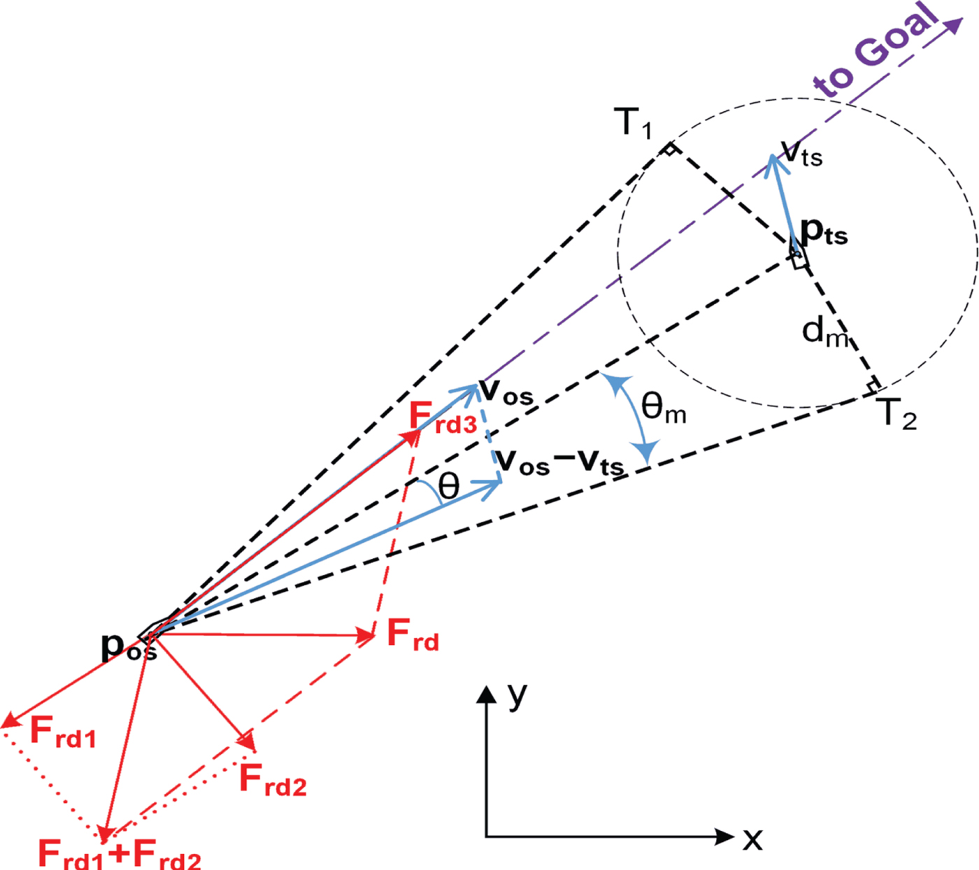
Figure 4. Modified repulsive force for a dynamic TS.
For an emergency CA action, that is, TSs in the EZ, the forces of turning left or turning right are chosen according to the minimum time to avoid collision. F rd1, F rs1 and F re1 are related to the relative positions of the OS and TSs, and they will keep the OS away from the TS in the corresponding conditions.  $\overrightarrow{n_{ot}}$ is the unit vector pointing to any TS from the OS, and
  $\overrightarrow{n_{ot\perp}}$ is a unit vector that is perpendicular to
  $\overrightarrow{n_{ot}}$ (see Figure 2). F re2 will automatically make the OS avoid danger from the right or left side of P ot depending on which side of the P ot line the vector V to is in. F rd2 always makes the OS alter course to starboard at a range of CR based on seafarers' practice, as the appropriate passing side for each encounter is determined by the COLREGS. F rd3, F rs3 and F re3 force the OS to move towards the goal.
Based on the calculation of the attractive and repulsive forces, the total virtual force is obtained by:
 $$F_{total}=F_{att}+F_{rep} $$
As there are multiple TSs, the repulsive force is given by:
 $$F_{rep}=\sum_{{\rm s}=1}^{n}F_{rep_{{\rm s}}} $$
where  $F_{rep_{\rm s}}$ is the repulsive force generated by the s-th TS, and n is the number of encountered TSs. Therefore, the OS will take CA actions under the total resultant F total for different conditions and reach the goal, although the goal is near a stationary obstacle. A flow chart of the modified APF method is given in Figure 5.

Figure 5. Flow chart of the modified APF method.
4. MODEL OF THE SHIP'S MOTION
A model of the ship's motion is simulated on the horizontal plane. All TSs can be set to change their course at any moment. Moreover, the process of CA at sea is described with the use of a kinematic model of ship motion, where state variables and control values are represented in the following forms:
 $$\eqalign{P_{os} & =\lsqb p_{ij}\rsqb _{m\times 2} \cr \dot{p}_{i1}^{os} & =V_{os}\times\cos\psi_{os}\lpar t\rpar \cr \dot{p}_{i2}^{os} & =V_{os}\times\sin\psi_{os}\lpar t\rpar } $$
 $$\eqalign{P_{ts} & =\lsqb p^{ts}_{ij}\rsqb _{k\times 2} \cr P_{tsi} & =\left[\matrix{ p_{\lsqb n\lpar i-1\rpar +1\rsqb 1}^{ts} & p_{\lsqb n\lpar i-1\rpar +1\rsqb 2}^{ts} \cr \vdots & \vdots \cr p_{\lpar n\times i\rpar 1}^{ts} & p_{\lpar n\times i\rpar 2}^{ts}}\right]\cr V_{ts}&=\lsqb v_{ij}\rsqb _{{\rm n}\times 2} \cr \dot{P}_{tsi} & =V_{ts}} $$
where i = 1,2,…,m is the i-th time step, k is the product of m and n, P os and P ts are coordinates of the OS and TS position, respectively, and V os and V ts are velocities of the OS and TS, respectively.
The course changes for TSs can be activated at some designated time step, which is calculated by the following formulae:
 $$a=\hbox{sgn}\lpar \hbox{rand}\lpar 1\rpar -0{\cdot}5\rpar \times\Delta\psi_{ts} $$
 $$\hbox{A}=\left[\matrix{ \cos a & \sin a \cr -\sin a & \cos a}\right]$$
 $$V_{ts-new}=V_{ts}\times A $$
where Δψ ts is the maximum value of course alteration of the TS at one time step, α is used to determine the random magnitude and sign of the course alteration, A is the transformation matrix for changes of course and V ts−new is the new course of the TS at the designated time step. The CA action of the TS is assumed to maintain course and speed (it does not give way when it should), or it alters its course into a worse situation. Certainly, a coordinated CA action can also be chosen in simulations.
The OS maximum turning angle to port or starboard at one time step is [-maxturn, maxturn]. To approach this issue, let ψ f be the angle of the total force F total, and ψ os be the heading of OS at the (i-1)-th time step. Then, the preliminary steering angle Δψ p is given by:
 $$\Delta\psi_{{\rm p}}=\psi_{{\rm f}}-\psi_{{\rm os}} $$
The final steering angle Δψ os (see Figure 5) can be determined by:
 $$\Delta\psi_{{\rm p}}=\left\{\matrix{\Delta\psi_{{\rm p}}-2 \pi \hfill & \hbox{if}\, \Delta\psi_{{\rm p}} \gt \pi \hfill \cr \Delta\psi_{{\rm p}}+2\pi \hfill & \hbox{if}\, \Delta\psi_{{\rm p}} \lt - \pi \hfill }\right. $$
 $$\Delta\psi_{{\rm os}}=\left\{\matrix{\min\lpar maxturn\comma \; \Delta\psi_{{\rm p}}\rpar \hfill & \hbox{if}\ \Delta\psi_{{\rm p}}\geq 0 \hfill \cr \max\lpar -maxturn\comma \; \Delta\psi_{{\rm p}}\rpar \hfill & \hbox{if}\ \Delta\psi_{{\rm p}} \lt 0 \hfill }\right. $$
The desired heading of the OS ψ os at the i − th time step is given by:
 $$\psi_{{\rm os}}\lpar i\rpar =\psi_{{\rm os}}\lpar i-1\rpar +\Delta\psi_{{\rm os}} $$
The dynamic properties of the OS are taken into account by considering the time needed for a ship to execute the calculated manoeuvre, that is, course change (Lazarowska, Reference Lazarowska2017). The course change should be large enough in a shorter period of time to ensure the avoidance manoeuvre is obvious to other parties. Therefore, the configuration of the parameters of maxturn and the time step are used to reflect the dynamic properties of the OS. This mainly depends on the available rudder angle (≤35°), the speed v os, the loading condition and the delay of turning for a specific OS. For some large vessels, if 5° is the maxturn and 15 s is the time step, the total turning angle for 2 minutes will reach 40° (satisfying Rule 8b). However, a slightly bigger maxturn with a shorter time step could be selected for more manoeuvrable vessels, which is also compliant with the “readily apparent manoeuvre” clause. It is therefore desirable to achieve a smooth path by incorporating the dynamic properties, including the turning abilities of the OS.
Meanwhile, this path contains the desired heading at any given point in near real-time. This is convenient for modelling the tracks and designing an automatic pilot. To control the course of the ships, slide mode controllers and a Proportion Integration Differentiation (PID) control system may be used. Complex modelling for track keeping and course controlling are beyond the scope of this paper.
5. RESULTS AND ANALYSIS
Extensive simulation cases were implemented using MATLAB software. The simulations considered COLREGS compliance and a wide range of cases, from a single TS avoidance to multi-ship avoidance, and from single predictable TS trajectories to complex and random TS trajectories, as well as stationary obstacle avoidance.
5.1. Experimental conditions and explanations
The calculations were conducted using a PC with an Intel Core i5 3230 m 2·6 GHz processor, 6 GB RAM, and a 64-bit Windows 7 Professional operating system. The following values for the parameters were used in the presented simulation tests: ε = 3, 000, η d = 2, 000, η s = 300, 000, η e = 2, 000, τ = 0 · 3 nautical mile (nm), R os = 0 · 5 nm, d safe = 0 · 5~1 nm (1 nm is selected for open water), ρ o = 3~5 nm, maxturn = 5°, and time step = 15 seconds.
The simulation results are illustrated in multiple figures, representing snapshots of situations. A two-dimensional Cartesian coordinate system presents the distance in nautical miles (nm); the vertical axis in the positive direction shows North 000°, and the horizontal axis in the positive direction is 090°. The following symbols and colour codes are applied:
• The black curve is the OS trajectory, and its starting point and goal point are indicated by the red square and blue triangle, respectively. In addition, the OS heading data at every time step is plotted, to easily find the course alteration points.
• The paths of multiple TSs, including stationary obstacles, are identified by corresponding TS numbers and different colours.
• The relative bearing of each TS and the range (scope 0~6 nm) between the OS and any TS at each time step is chosen to display with various colours.
• All the paths are marked at regular intervals, for example, 60 time steps.
5.2. Collision avoidance with one TS
Overtaking, Head-on, and Crossing encounters are presented in this paper, see Figures 6–8(a), 8(b) and 8(c), and the reactive avoidance actions of the OS replying to the uncoordinated behaviours of the TS are illustrated in Figures 6–8(d), 8(e) and 8(f). The initial configuration of these simulations is described in Table 3, which contains the start positions (p ts), velocities (v ts), and radii (R ts) of the TSs. For example, (−8, 8) for v ts means that the velocities on the x-axis negative direction and y-axis positive direction are 8 kn and 8 kn, respectively. The OS's start point (0, 0) and destination (10, 10), as well as initial course 045° and speed 12 kn are designated. The simulation results, including the course changes and distances from the TS at the action time for the OS, the final Distance of Closest Point of Approach (DCPA), and the total run time of each simulation are also described in Table 3.
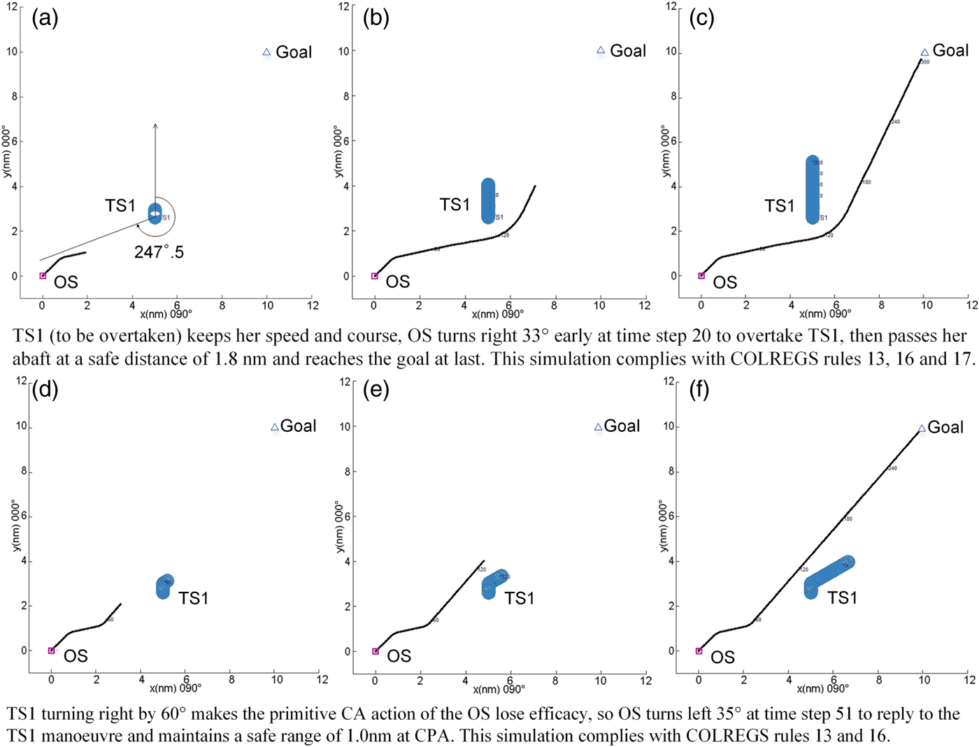
Figure 6. Single-TS Overtaking encounter simulation.
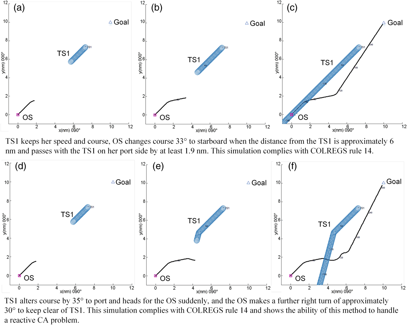
Figure 7. Single-TS Head-on encounter simulation.
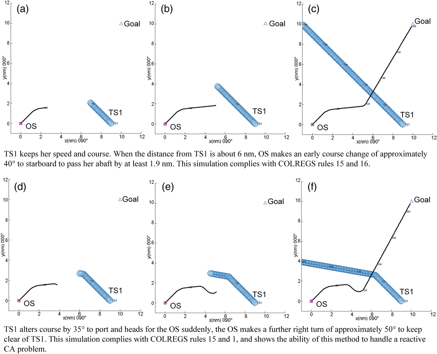
Figure 8. Single-TS Crossing encounter simulation.
Table 3. Initial inputs and simulation results for three typical encounters

It can be seen clearly that the OS's behaviour complies with COLREGS Rules 13–17, and the computation time is very low (no more than 130 milliseconds) to satisfy the real-time requirement for CA or path planning online.
5.3. Collision avoidance with multiple obstacles
Two cases were chosen for this scenario.
Case 1 presents an encounter between the OS and four moving TSs and two static obstacles. The initial input for OS is no change. The initial configurations for the TSs are described in Table 4 and an uncoordinated course alteration (30°) of TSs are considered. Figures 9(a)–(h) indicate the temporary positions at the selected step and the trajectory history of all TSs. Figures 9(h1)–(h3) illustrate the distance between the OS and any TS, the relative bearings of the TSs, and the heading of the OS at each time step.

Figure 9. Graphical solution of case 1. Video files are available as Supplementary Material.
Table 4. The initial inputs for TSs at case 1

In Figure 9(a), initially the OS moves towards the goal along the nominal path. It can be observed that a TS4 head-on situation and a TS3 crossing situation from starboard are developing. However, the distance between the OS and TS3 and even TS4 are so large (more than 6 nm) that CA algorithms are considered to not apply according to the threshold CR. When the distance between them reaches the CR (at step = 12 in Figure 9(h)) first for TS3, the OS makes a course change 30° to starboard to avoid the two risks.
In Figure 9(b), TS3 and TS4 change their courses to port to intercept the OS trajectory, which is deemed as an uncoordinated CA action. Therefore, the OS makes a further course change of 35° to starboard (at step = 60) to avoid a collision with TS3, although it will lead to a larger deviation from the planned trajectory. This shows that the method is able to successfully handle and quickly react to the presence of obstacles with an unpredictable course change.
In Figure 9(c), after passing TS3 at safe range 1·4 nm, the OS returns to the planned route. Note that TS4 is arriving from the port side after turning left, and the OS has the right to stand on. This stand-on behaviour means that it takes the OS far away from the planned trajectory. However, this is compliant with the COLREGS and is safe.
In Figure 9(d), after passing at a safe distance (1·2 nm according to d m) in front of TS4 (according to CC: θ < θ m), the OS makes a sharp turn 51° (at step = 115) to port to avoid collision with the static obstacle TS1. Finally, TS1 is passed at 1·4 nm (see Figure 9(h1)) on the OS's starboard side.
In Figure 9(e), TS2 is ahead of the OS. Meanwhile, TS5 is arriving from the port side such that it is a give-way ship. In this scenario TS5 does not respect its responsibility to give way and the OS makes a course change (approximately 31° at step = 155) to starboard to avoid collision with the TS5 and to avoid a hazardous situation if TS5 alters course to starboard in compliance with its responsibility to keep clear according to COLREGS. In addition to the stationary obstacle, TS2 can be passed at a safe distance (approximately 1·3 nm, see Figure 9(h1), blue line) on the OS's port side.
In Figure 9(f), after clearing TS2 and TS5, the OS turns left 30° (at step = 190) towards the goal, taking into account the influence of TS6. Since TS6 is approaching from the port side and the DCPA (1·7 nm, see Figure 9(h1), brown line) is enough to pass clear, the OS stands on and moves to the goal without any collision risk, until reaching the goal at step = 315.
Case 2 contains a more complex situation in which 11 TSs have random changes in course and five TSs are stationary obstacles, as shown in Figure 10. The initial configuration is shown in Table 5. The OS's start point is set to (1, 1) and the other parameters remain the same.

Figure 10. Graphical solution of case 2. Video files are available as Supplementary Material.
Table 5. The initial inputs for TSs of case 2.

In Figures 10(a) and 10(b) the OS alters course 50° to starboard to pass abaft TS8, meanwhile avoiding the close-quarters situation with TS1. In Figures 10(c) and 10(d), after passing clear of TSs #12, 7, 3 and 8 at a safe distance of 1 nm, the OS makes a large starboard turn of 90° to manage the uncoordinated behaviours of TS2 and passes clear at 0·9 nm. In Figures 10(e) and 10(f), the OS avoids the static obstacle of TS #16, and 11, then reaches the goal, although TS11 is near the goal.
Simulations show that the OS can make a collision-free path with multiple TSs making unpredictable course changes and manage the reactive CA problem. The computational time is also very short (140~200 milliseconds, that is, ms at 50 repetitions of calculations) and is invariant in almost every simulation. Further, it does not obviously increase with an increasing number of TSs or their random motion. Meanwhile, the solution for the same situation is also deterministic for every run of the calculations. As the algorithm is based on a simple deterministic structure with regard to the field and gradient theory, it is algorithmically complete in such a way that it will generate the exact solution (if it exists). This is because no random variables are involved in the computation and the outputs from the algorithm are entirely consistent and predictable for the same known conditions. Additionally, there is no feasible solution in the simulations for some extreme situation where the TS suddenly alters course to a worse condition and rushes at the OS at a critical close range. In this scenario a collision may be inevitable even in a real situation due to the limitation of the manoeuvrability and reaction time of the OS.
Due to the maxturn limit, the heading plot includes some small fluctuations, that is, the small course changes. A smooth heading line is re-plotted using one-dimensional MATLAB median filtering (see the magenta solid line in Figures 9(h3) and 10(h2)). Compared with the original heading data (blue dotted line), the new heading line preserves the substantial course changes and is smoother than before so that it is feasible for the ship. By inputting the new heading data, the new planned path can also be obtained (see the magenta line in Figures 9(g) and 10(g)), which almost coincides with the original planned path (the black line) and does not influence the collision avoidance effect. Other small course changes are eliminated by adjusting the parameter d safe, with a larger d safe ensuring that the course changes are readily apparent.
6. CONCLUSIONS
A real-time path planning method based on a new modified APF model is presented in this paper. Simulations illustrate that this method is well-suited for automatic path planning and collision avoidance in a complex environment, where static and dynamic obstacles occur. Additionally, it is compliant with Rules 13–17 of COLREGS for power-driven vessels and shows the potential to address the extreme or emergency multi-ship collision situations mentioned by Xue et al. (Reference Xue, Clelland, Lee and Han2011) and Perera et al. (Reference Perera, Carvalho and Soares2011) in their proposed future work. The proposed method is robust in the uncertainty of TS strategies, such as unpredictable changes of course in the solution finding process. In addition, a smoother path is achieved by considering the dynamics of the OS.
The strength of the approach appears in the capability to plan a collision-free path in a very short time (millisecond level) for the OS. Additionally, the computational time is barely affected by the number of obstacles and the random course changes of the TSs.
The presented simulation results prove the advantages and effectiveness for real time path planning using the proposed method. Due to the deterministic and acceptable solution derived for the complex collision avoidance task, a very low and almost constant computational time for every scenario, repetition and robustness for the uncertainty of other ship's behaviours, it can be applied to an on board anti-collision decision-making system and promotes the automation level of a USV or an autonomous ship.
The method can be further refined by considering speed reduction behaviours and more accurate ship dynamics, as well as the uncertainty of environmental disturbances and area-based obstructions.
ACKNOWLEDEGMENTS
This work was financially supported by Traffic Youth Science and Technology Talent Project (Grant No. 36260401), Science and Technology Program of Yunnan Communication Department (Grant No. YunJiaoKe2013(A)01), Natural Science Foundation of Liaoning Province of China (Grant No.201602081), and the Fundamental Research Funds for the Central Universities [No.3132018306].
Supplementary material
The supplementary material for this article can be found at https://doi.org/10.1017/S0373463318000796.


