1. INTRODUCTION
The operation of the new applications for driving assistance being introduced in road vehicles is based on information processing of the vehicle, the driver, the route and the environment. For many, digital maps involve expanding the visual horizon beyond what is perceived by the driver and the onboard sensors (Reichart et al, Reference Reichart, Friedmann, Dorrer, Rieker, Drechsel and Wermuth1998; Venhovens et al, Reference Venhovens, Bernasth, Löwenau, Rieker and Schraut1999; Njord et al, Reference Njord, Peters, Freitas, Warner, Allred, Bertini, Bryant, Callan, Knopp, Knowlton, López and Warne2006; Wevers and Lu, Reference Wevers and Lu2007; Jiménez and Naranjo, Reference Jiménez and Naranjo2009). However, to exploit its potential it is necessary to define a specification of accuracy and detail in these maps and positioning systems to higher levels than those currently used for navigation purposes (Noronha and Goodchild, Reference Noronha and Goodchild2000; Baum, Reference Baum2003; Organisation for Economic Co-operation and Development, 2003; T'Siobbel and van Essen, Reference T'Siobbel and van Essen2004; Lu et al, Reference Lu, Wevers, van der Heijden and Heijer2004; Pandazis, Reference Pandazis2006; Jiménez et al, Reference Jiménez, Aparicio and Páez2008; Jiménez and Naranjo, Reference Jiménez and Naranjo2009). In this regard, of particular interest are the recent findings developed within the eSafety working group on digital maps (eSafety Forum, 2005) and the final results of the Map&ADAS sub-project of the PREVENT EU-funded Integrated Project (T'Siobbel et al, Reference T'Siobbel and van Essen2004).
Two lines of research appear: first, the development of digital maps; and secondly the positioning of the vehicles on those maps. Nowadays, in the first case, a solution is to use digitised paper maps or aerial photographs (Bendafi et al, Reference Bendafi, Hummelsheim, Sabel and van de Ven2000; Miles and Chen, Reference Miles and Chen2004), but when accuracy needs to be combined with fast measurement or when highly detailed maps are required, the solution is to use a datalog vehicle (Yerpez and Ferrandez, Reference Yerpez and Ferrandez1986; EDMap Consortium, 2004). On the other hand, in the second case, GPS positioning is the most widespread solution. Hence, focusing on onboard measurement and positioning systems, two large groups can be distinguished; GPS positioning and inertial measurement systems.
GPS positioning is not robust enough and metric accuracy cannot be guaranteed for on-the-lane positioning, as some of the new ADAS applications require (Jiménez and Naranjo, Reference Jiménez and Naranjo2009). Furthermore, the satellite signal can be lost in some circumstances (driving through tunnels, between high buildings, etc) and important information for new digital maps such as the super-elevation rate cannot be obtained in a direct and accurate way. Despite the preceding ideas, some authors have used GPS positioning to obtain the road geometry. Among these, in Castro et al (Reference Castro, Iglesias, Rodríguez-Solano and Sánchez2006), the cruising speed is approximately 80 km/h with a 1 Hz sampling frequency, which gives points that are spaced 20 metres apart. They use the mean and standard deviation of the lane width measurement when measuring the same route using different lanes, as an indicator of accuracy. In Ben-Arieh et al (Reference Ben-Arieh, Chang, Rys and Zhang2004), the authors also use a GPS receiver with a 1 Hz sampling frequency and a vehicle speed of 100 km/h. In both cases the filtering and elimination of erroneous points is required. In Transportation Research Board (2002), GPS positioning signal is used to integrate the road geometry information into a GIS. In order to increase accuracy of GPS positioning, differential correction techniques can be used. This correction is based on the use of a second GPS unit, whose position is accurately known, so errors can be estimated and can be extrapolated to the measures of the mobile GPS receiver in the vehicle. In Naranjo et al (Reference Naranjo, Jiménez, Aparicio and Zato2009), different types of differential corrections are described and tested. The quality of positioning is measured following the standard GPS NMEA convention: type 4 or fixed for centimetric accuracy, type 5 or floating for sub-metric accuracy and type 1 or autonomous (the device is positioning without differential correction) for metric accuracy (error of 10–15 m maximum). In most cases, results were not completely satisfactory because: 1) virtual base stations do not guarantee high signal quality all the time, and 2) proprietary base stations can overcome previous limitations but their small range means that accurate results can only be obtained near the station and corrections are not possible too far away from it. In both cases, the main problem is that the greater the distance between the two GPS units, the bigger the positioning error is, so that distance is limited to tens of kilometres. Despite previous considerations, in Imran et al (Reference Imran, Hassan and Patterson2006) differential GPS with a 0·1 Hz sampling frequency is used in order to increase accuracy in positioning.
Previous solutions cannot solve signal degradation or signal losses under adverse conditions (urban environments, trees, high walls near the road, etc). For many years inertial measurements systems have been seen as a solution to minimize previous limitations by combining both positioning methods (e.g. Zhang and Gao, Reference Zhang and Gao2008). These inertial systems do not have the problems of signal losses and can provide data as super-elevation rate in a direct way. Drakopoulos and Örnek (Reference Drakopoulos and Örnek2000) use speed measurements and a gyroscopic sensor to deduce the horizontal alignment. Measurements are taken every 16 metres and the angular precision is 1°, which can lead to significant errors. Subsequently, a distinction is made between straight lines and curves based on the variation of the yaw angle. The problem arises when accuracy requirements increase, so it is necessary to analyze whether this system is reliable for accurate digital map development and on-the-lane positioning because of the cumulative error that inertial systems present (Jiménez et al, Reference Jiménez, Aparicio and Estrada2009). Borenstein et al (Reference Borenstein, Ojeda and Kwanmuang2009) set out a method to reduce the effect of gyroscopic platforms drift. A comparison of results using a differential GPS receiver and a low-cost 2D inertial measurement unit is presented in EDMap Consortium (2004) . Han and Wang (Reference Han and Wang2010) show the integration of GPS and reduced inertial navigation systems and propose a novel method for estimating position and speed. In this sense, the use of Kalman filtering is a very widespread solution in order to improve the positioning obtained using different measurement methods (Labrech et al, Reference Labrech, Boucher and Noyer2004; Rezaei and Sengupta, Reference Rezaei and Sengupta2007; Toledo-Moreo et al, Reference Toledo-Moreo, Zamora-Izquierdo, Úbeda-Miñarro and Gómez-Skarmeta2007; Xu et al, Reference Toledo-Moreo, Zamora-Izquierdo, Úbeda-Miñarro and Gómez-Skarmeta2008, Jwo and Lai, Reference Jwo and Lai2009). Lee and Jekeli (Reference Lee and Jekeli2009) implemented and compared four different filtering algorithms: the extended Kalman filter (EKF), the unscented Kalman filter (UKF), the unscented particle filter (UPF), and the adaptive unscented particle filter (AUPF). Baselga et al (Reference Baselga, García-Asenjo, Garrigues and Lerma2009) propose a data-filtering scheme to apply to inertial measurement systems raw data prior to the integration with GPS. In other approaches, neural networks are used to integrate GPS and inertial measurement systems (Jwo and Huang, Reference Jwo and Huang2004; Lee and Jekeli, Reference Lee and Jekeli2010). Xu et al (Reference Xu, Li, Rizos and Xu2010) show the integration of the least squares support vector machine and Kalman filter. Other limitations such as not considering an absolute reference are easily solvable and they do not entail additional problems.
Furthermore, although high-cost equipment (similar to the equipment tested in Naranjo et al, Reference Naranjo, Jiménez, Aparicio and Zato2009) can be used for digital maps development, they cannot be used for vehicle positioning because they are not affordable for consumers. The performance of low-cost measurement systems that could be installed in mass-production vehicles should be evaluated in order to assess whether they fulfil the specifications of new ADAS applications, some of which require accurate on-the lane positioning (Kwon et al, Reference Kwon, Kim and Betts2003; Alexander et al, Reference Alexander, Cheng, Donath, Gorjestani, Newstrom, Shankwitz and Trach2005). In marine applications, low-cost single-frequency OEM GPS receivers for high-accuracy kinematic positioning have been tested (Alkan and Saka, Reference Alkan and Saka2009) but road environments can be more restrictive and signal degradation problems could be more frequent. Taking previous considerations into account, this paper presents an experimental analysis of performance of low-cost autonomous GPS receivers under normal driving conditions. Furthermore, we study to what extent the cumulative errors of inertial systems are admissible by new ADAS accuracy requirements. This study is carried out from a theoretical point of view using uncertainty propagation law and results are checked using test data of high- and low-performance equipment.
2. OBJECTIVES, METHOD AND EQUIPMENT
Nowadays, digital map development can justify using high-performance equipment (differential GPS receivers and high accuracy inertial systems), but present applications of vehicle positioning do not justify their surcharge. For this reason, it is useful to analyze the performance of low-cost inertial systems in determining vehicle trajectory under normal driving conditions. The main objectives of this paper are:
• To determine results degradation when low-performance measurement equipment is used under real driving conditions and to analyze whether its use is viable on new ADAS applications that require on-the-lane positioning.
• To use theoretical and experimental approaches to determine the cumulative error when using high-performance inertial measurement systems for vehicle positioning or for digital map development, and to establish a travelled distance limit in order to observe new ADAS specifications that require on-the-lane positioning when GPS signal is lost or degraded.
• To analyze the possibility of obtaining accurate results by combining both sources of information (GPS and inertial systems).
An extensive test plan has been carried out, comparing high-performance systems with low-performance ones. These tests include trajectories on the University Institute for Automobile Research test track and routes along rural roads that combines a wide range of operating conditions. The following instrumentation is used:
• High performance systems:
∘ RTK DGPS Topcon GB-300 receiver with an update frequency of 10 Hz and the possibility of using American GPS and Russian GLONASS.
∘ Inertial measurement system that is composed of a Correvit L-CE-non-contact speed sensor and a RMS FES 33 gyroscopic platform.
• Low-performance systems:
∘ Astech G12 receiver in autonomous mode with a 10 Hz update frequency.
∘ Garmin GPS eTrex H receiver in autonomous mode with a 1 Hz update frequency.
∘ Xsens MTi-G that includes a gyroscopic platform and a GPS receiver with an update frequency of 1 Hz.
3. PERFORMANCE ANALYSIS OF LOW-COST GPS RECEIVERS
The performance of GPS receivers has been tested under different operating conditions. RTK DGPS receiver results are used as reference data, so when type 4 accuracy level is achieved, the complete difference can be assigned to the other system, but in the other cases, that difference should be divided.
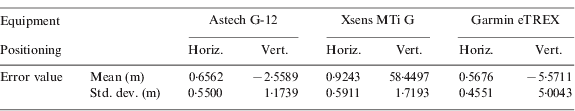
Firstly, tests were performed on the test track. Figure 1 shows one of the trajectories and the comparison between all the GPS receivers involved in the tests. In these tests, type 4 accuracy level is almost guaranteed for the DGPS, and it can be seen that differences are admissible for the use of all receivers in new ADAS applications that require on-the-lane positioning (Table 1). Larger differences arise when the vertical magnitude is considered. In this case, DGPS receivers present a more accurate and repetitive behaviour. However, this situation is not very relevant because vertical positioning is not crucial, in general, and the combination of horizontal positioning and accurate digital maps can provide that information if necessary.

Figure 1. Comparison of trajectories obtained by different GPS receivers.
Table 1. Differences in the GPS positioning during the test on the test track (Reference value: results of DGPS Topcon GB-300).
In any case, in more realistic trajectories, differential correction does not provide type 4 accuracy level all the time. In some cases, the distance percentage of high accuracy is quite low (Naranjo et al, Reference Naranjo, Jiménez, Aparicio and Zato2009). For this reason, when this accuracy level is not achieved, the difference between receivers cannot be ascribed to only one of them. Furthermore, the analysis of the signal recovery time after a signal loss is interesting, because inertial systems should be used during that time and cumulative error should be taken into account.
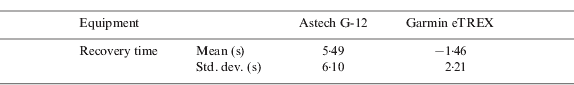
Figure 2 shows a trajectory that combines urban and rural areas, and different areas are distinguished. Table 2 shows the signal recovery time referred to the time required by the Topcon GB-300 receiver (negative times mean a higher recovery speed of the analyzed receiver). There are not clear data tendencies but it was found that the low-performance Garmin eTREX receiver can recover the signal more quickly but it is also prone to short losses.

Figure 2. Test trajectory that combines urban and rural areas.
Table 2. Signal recovery time after a signal loss referred to the time required by the Topcon GB-300 receiver.

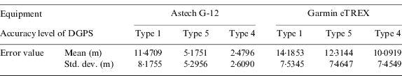
Table 3 contains the positioning differences between receivers in the different possibilities of accuracy of the DGPS receiver. As can be seen, these differences are higher when type 4 accuracy level is not achieved, because of the lower quality of the reference and the worse operating conditions of every receiver. According to the results obtained with the two low-performance receivers, only the Astech G 12 receiver can guarantee on-the-lane positioning on those road stretches where the DGPS achieves the highest accuracy level. In other situations, the measurement uncertainty is larger than the lane width and the low-cost Garmin eTREX receiver cannot provide results accurate enough even under good operating conditions. It should be noted that in these tests the Xsens MTi G equipment has not been considered because it comprises the GPS receiver and the gyroscopic platform and it combines both when signal losses occur.
Table 3. Differences in the GPS positioning during the test in normal driving conditions (Reference value: results of DGPS Topcon GB-300).
4. USE OF INERTIAL MEASUREMENT SYSTEMS
4.1. Theoretical approach
Using inertial measurement systems, the trajectory can be computed by means of the following equations:


where (x, y) are the Cartesian co-ordinates, v is the cruising speed, Δt is the time between the two measurements and θz is the angle drawn around the Z-axis defined in the mobile system of the datalog vehicle (the X axis is aligned along the longitudinal axis of the vehicle, the Z is the vertical and Y forms a right-handed system with the other two).
The main problem of this method is that the error committed in this measurement is cumulative, mainly because of the gyro drift. It is necessary to evaluate the magnitude of this error. From a theoretical point of view, the uncertainty of results using inertial systems can be evaluated applying the law of propagation of uncertainty (Taylor and Kuyatt, Reference Taylor and Kuyatt1994; European co-operation for Accreditation, 1999). The global uncertainty of an indirect output variable α defined as α=f(β1, β2,…, βN) is given by the following general expression:

where u(βi) is the uncertainty component of the input variables, u(βi, βj) is the covariance when input variables are correlated and c i is the sensitivity coefficient of each uncertainty component.
When applying the previous equation to the calculation of the x and y coordinates' uncertainty, it may be assumed that the input quantities are not correlated because they come from different equipment, so the terms involving covariances are zero and the previous equation can be applied, only taking into account the uncertainties of the input variables (longitudinal speed, yaw angle and time interval).
Depending on the application for which the digital map or the vehicle positioning is going to be used it is critical to establish an admissible upper limit of committed error. Assuming the uncertainty of measurement in the yaw angle and the time between the two measurements are constant and the speed uncertainty is linear in respect of the speed value, we can consider that:
Using these assumptions in the expression of the sum of uncertainties of the X and Y coordinates, the following result is achieved:

where it has been assumed that the time between the two measurements is constant.
In order to find a higher limit for the uncertainty, a constant maximum speed is considered, giving:

where d is the distance travelled.
From this equation it is deduced that the distance that can be travelled without the figure for uncertainty exceeding an admissible limit u 2(x)+u 2(y)⩽L 2 is equal to:
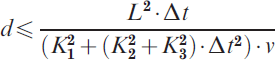
It should be noted that the previous equation provides the evaluation of the uncertainty in the measurement of the road geometry before doing the measurement (a priori evaluation), so applied means can be analyzed in order to assess whether they are suitable for the specifications. Hence, for example, ADAS applications that require on-the-lane positioning enforce an upper bound for uncertainty in the position as equal to the lane width and this implies a very restrictive situation as regards the maximum distance that can be travelled using only inertial systems for positioning. Figure 3 shows the calculated distance considering the instrumentation used. This distance depends on the speed and the sampling rate, apart from the characteristics of the instrumentation. Note that the distance increases when reducing the speed and presents a maximum value on a specific rate that depends only on the characteristics of the instrumentation (in this case, near to 20 Hz). Finally, it should be taken into account that the upper limit increases in a quadratic way when increasing the positioning tolerance and this fact significantly reduces the demands on the instrumentation of the datalog vehicle.

Figure 3. Dependence of the maximum distance on the travelling speed and the sampling rate.
4.2. Experimental approach (comparison between high- and low-performance equipment)
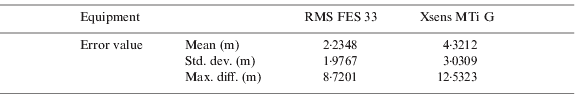
Tests using the different inertial systems were carried out on a test track. Three laps were completed with a total length of 1581 metres. The trajectory was calculated using equations (1) and (2). Results are shown in Figure 4 and Table 4, in which DGPS data can be taken as the reference ones because type 4 accuracy level is maintained along the whole test. It can be seen that cumulative errors with low-performance systems are significantly larger than with high-performance ones.

Figure 4. Comparison of trajectories using inertial measurement systems.
Table 4. Differences in the positioning using inertial systems (Reference value: results of DGPS Topcon GB-300).

It should be noted that, when applying equation (9) to the RMS FES 33 gyroscopic platform high performance inertial system, 231·83 metres is the upper limit of the distance travelled for guaranteeing on-the-lane positioning that can be travelled using only the inertial measurement system assuming a correct positioning at the starting point and test operating conditions. Furthermore, the theoretical approach provides an estimation of the maximum error in the whole trajectory (9·14 metres). There is a difference of 4·82% when comparing this figure with the experimental one, and we should keep in mind that the theoretical formula provides an upper limit and overestimates the error.
5. COMBINATION OF GPS AND INERTIAL MEASUREMENT SYSTEMS
The combination of GPS positioning and inertial sensors is a widespread solution to deal with the limitations of each system separately, as previously mentioned. The developed algorithms for data fusion are based on determining the confidence level of each measure. Taking into account the satisfactory results of DGPS when type 4 accuracy level is achieved, it should be analyzed in which situations inertial sensors can improve results.
Two extreme situations can be distinguished when using DGPS receivers (only the first one can be applied to GPS receivers working in autonomous mode): 1) the inertial measurement system is used only when the GPS signal is lost; 2) the inertial measurement system is used when GPS accuracy is degraded. Of course, Kalman filters consider intermediate situations. The first solution can also be used with GPS receivers working in autonomous mode, but taking into account that the last point before GPS signal is lost and the first point after recovery do not usually present type 4 accuracy level, quite large uncertainty in GPS positioning is expected. For this reason, it could be a better solution to use inertial positioning in the road stretch where accuracy degrades and not to wait until the signal is lost, but, in this case, longer distances should be covered using inertial measurement systems, so a compromise is required.
In order to compare the results provided by both the extreme situations previously stated, tests have been carried out in urban and rural areas using the Correvit L-CE-non-contact speed sensor, the RMS FES 33 gyroscopic platform and the DGPS Topcon GB-300 receiver that can reach centimetric accuracy under certain conditions. The performance analysis is carried out comparing the final point N of the path computed using the inertial system with the GPS positioning, considering that the initial point of this stretch is taken as the origin. The error is then given by:
Figure 5 shows differences in the final points of road sections between the positioning of GPS signal and the positioning obtained using inertial measurement systems in the two situations. As can be seen, the consideration of a more reliable starting point for calculation using inertial measurements improves results significantly, despite the fact that the distance travelled using only the inertial measurement system is greater in this second situation. Of course, a compromise should be found between the relative error and the distance in order to minimize the cumulative error, because, in some cases, the recovery of type 4 GPS signal can need more time than expected and the distance travelled can increase significantly.

Figure 5. Positioning error using the inertial measurement system when GPS signal is lost or degraded.
More specifically, in the first case, errors of 6% of the distance travelled without GPS signal are found (average value and standard deviation of 3·2±1·1%) but it should be noted that we cannot say if the first difference is caused by the cumulative error of the inertial system or the GPS signal. On the other hand, in the second case, previous uncertainty is not present because centimetric GPS accuracy is guaranteed and discrepancies are around 0·9±0·4%, a lower value than in the first case owing to the fact that the influence of GPS errors has been removed. These results are coherent with conclusions derived from equation (9) when calculations are carried out when GPS signal accuracy is degraded, because lower distances than the calculated upper limit for guaranteeing on-the-lane positioning always provide errors lower than the lane width. However, this does not occur when using the inertial system data when the GPS signal is lost because signal degradation before and after signal losses lead to very high uncertainty values.
In the case of using low-performance equipment, the upper distance limit is outstandingly reduced if worse GPS accuracy level is considered for the starting point (for example, when differential correction is not used, a situation that is quite common) or higher uncertainty inertial equipment is used, so this makes non-viable the use of this kind of system during more than 5–6 seconds in ADAS applications that require high accuracy level of vehicle positioning. These results can be extrapolated to other tests because test conditions (road type, road surroundings, etc) do not have significant influence on the results provided by the inertial measurement systems.
6. CONCLUSIONS
When talking about the positioning of vehicles, two aspects must be considered: the positioning itself and the digital map development on which this positioning is applied. The accuracy requirements for new ADAS applications have implications for both of them and levels of accuracy and detail should be similar to achieve the objectives. However, it can be assumed that the construction of the digital map is more restrictive because it requires a greater depth of some variables such as super-elevation and ramps. In addition, providing detailed mapping can reduce the effect of errors in positioning during vehicle movements. Another relevant topic that should be taken into account is that high-cost equipment is affordable for digital maps development but not for its implementation in mass-production vehicles, in which present assistance applications do not justify their surcharge.
DGPS appears to be a good solution that provides accurate results, but it is not robust enough and other complementary methods such as inertial measurement systems should be introduced. Furthermore, it is expensive so other solutions should be explored. Low-cost GPS receivers can provide enough accuracy for most of the ADAS applications, mainly on x and y coordinates, but not on the z- coordinate, in which errors are very high. It should be noted that this variable is useful for digital map development, but it is not completely necessary for vehicle positioning on them. GPS signal losses can be solved using inertial measurements. In this case, a theoretical approach based on the uncertainty propagation law for estimating the cumulative error is set out. Experimental data validated the formula that gives the maximum distance that could be travelled without exceeding a specific error limit.
According to the results obtained, in most GPS signal losses, better results were obtained if inertial measures were used not only in the GPS loss road section but in the complete stretch with degraded accuracy, despite the fact that longer distances were considered. However, despite being a better solution, it is necessary that this degradation should not take too much distance in order not to include significant cumulative errors. For this reason, a compromise criterion should be considered. But low-cost gyroscopic platforms involve large errors in yaw measurement, so they probably do not provide accuracy levels required by new ADAS applications that need on-the-lane positioning because cumulative error on x and y coordinates become inadmissible very soon, so they can only be used to locate vehicles when GPS signal losses are very short or low levels of accuracy in that positioning are required (for example, to know if a vehicle has taken a certain diversion inside a tunnel without distinguishing the lane it is travelling along).
ACKNOWLEDGMENTS
The work reported in this paper has been partly funded by the Spanish Ministry of Science and Innovation (SIAC project TRA2007-67786-C02-01 and TRA2007-67786-C02-02) and the CAM project SEGVAUTO.