


1. Introduction
With the rapid development of aerospace technology, high-altitude spacecraft are playing an increasingly important role in military and civilian fields, such as long-distance communication, meteorological detection, disaster warning, and lunar exploration (Ashman et al., Reference Ashman, Bauer, Parker and Donaldson2018a; Chai et al., Reference Chai, Wang, Yu, Wang and Li2018). Currently, the orbit determination of high-altitude spacecraft is mainly undertaken by the ground Telemetry, Track and Command (TT&C) network. This method has problems such as complex equipment, high maintenance costs, and poor survivability during periods of ground conflict or as a result of disasters, meaning that it cannot meet future development needs (Capuano et al., Reference Capuano, Botteron, Leclère, Tian, Wang and Farine2015; Jing et al., Reference Jing, Zhan, Lu, Feng and Ochieng2015). As an important space infrastructure and strategic resource, the global navigation satellite system (GNSS) has the characteristics of high real-time, strong autonomy, high precision and low cost, which can simultaneously meet the needs of multiple navigation tasks such as positioning, velocity measurement, timing, and attitude determination (Groves, Reference Groves2013; Wang et al., Reference Wang, Ji and Feng2014). Using GNSS to provide an autonomous navigation service for high-altitude spacecraft can reduce dependence on the TT&C network, simplify navigation equipment and improve navigation precision. Therefore, the autonomous navigation technology for high-altitude spacecraft based on GNSS has important application value.
In order to verify the feasibility of autonomous navigation technology based on GNSS for high-altitude spacecraft, many flight tests have been carried out by research institutions in various countries. In 2001, the GPS receiver on the AMSAT OSCAR-40 satellite launched by the United States successfully tracked main lobe and side lobe signals at an orbital altitude of 58,800 km. Due to the insufficient number of visible GPS satellites, however, it failed to realise on-orbit real-time positioning (Moreau et al., Reference Moreau, Davis and Russell Carpenter2002). In 2013, the GPS receiver on the European Space Agency's GIOVE-A satellite realised on-orbit real-time positioning above the GPS constellation for the first time, at an orbital altitude of 23,300 km (Unwin et al., Reference Unwin, Blunt and Steenwijk2013). In 2014, the Chang'E 5-T1 lunar probe launched by China was equipped with a GNSS receiver compatible with GPS and GLONASS signals, and verification of the on-orbit flight test was carried out in both the Earth–Moon transfer orbit and the Moon–Earth transfer orbit (Wang et al., Reference Wang, Dong and Wang2015). In 2015, formation satellites carrying out NASA's Magnetospheric Multiscale mission were equipped with Navigator GPS receivers, which have the ability of fast acquisition of weak signals, and successfully realised the navigation solution at an orbital altitude of 76,000 km (Winternitz et al., Reference Winternitz, Bamford, Price, Russell Carpenter, Long and Farahmand2017). In 2016, SJ-17 launched by China was equipped with a high-sensitivity GNSS receiver compatible with the main lobe and side lobe signals of GPS/GLONASS/BDS, which was used to carry out the experimental verification of GNSS-based navigation technology in geosynchronous orbit (Gao et al., Reference Gao, Wang, Liu, Che and Zhang2017). Subsequently, China launched the TJS-2 satellite for the verification of on-orbit navigation based on GNSS in geostationary orbit (GEO) (Jiang et al., Reference Jiang, Li, Wang, Zhao and Li2018). In general, the GNSS-based autonomous navigation technology for high-altitude spacecraft is still in the feasibility exploration stage.
Only limited test data has been returned through flight tests and used to guide the development of GNSS receivers suitable for high-altitude space (this paper refers to the space above the GNSS constellation). So far, availability analysis is still an important means to understand the characteristics of GNSS signals in high-altitude space. Moreau (Reference Moreau2001) took the lead in analysing the characteristics of GPS signals in high-altitude space from the number of visible satellites, carrier-noise ratio, Doppler shift and geometric dilution of precision (GDOP). Dion et al. (Reference Dion, Calmettes, Bousquet and Boutillon2010) further considered the ionosphere loss, and analysed the improvement in availability of GNSS signals by compatibility with GPS and Galileo for a specific geosynchronous orbit user. In 2012, NASA proposed to use the minimum number of visible satellites, the lowest power of signal received and the pseudorange accuracy in measuring the availability of GNSS signals to the space service volume (SSV) in the altitude range from 3,000 km to 36,000 km (Miller and Moreau, Reference Miller and Moreau2012). Jing et al. (Reference Jing, Zhan, Lu, Feng and Ochieng2015) proposed an analytical methodology to characterise the minimum received power for the worst location, and defined the estimated position error to analyse the signal characteristics in the SSV. In 2018, a United Nations-coordinated report (UN Office for Outer Space Affairs, 2018) further revealed the potential of interoperable GNSS for improving the availability of main lobe signals in SSV through many cases. Although the formal definition of SSV ends at geostationary altitude, the availability of GNSS signals in higher altitude space has also received extensive attention (Ashman et al., Reference Ashman, Parker, Bauer and Essewin2018b). Many studies in the literature have examined the availability of GNSS signals at lunar altitude from different aspects, including duration of the time intervals in which four GNSS signals are acquired simultaneously (Palmerini et al., Reference Palmerini, Sabatini and Perrotta2009), the influence of lunar occultation on availability of GNSS signals (Silva et al., Reference Silva, Lopes, Peres, Silva, Ospina, Cichocki, Dovis, Musumeci, Serant, Calmettes, Pessina and Perello2013), and the synergies between GNSS signal/navigation processing and other navigation sensors (i.e., accelerometers, optical camera, laser altimeter) (Manzano-Jurado et al., Reference Manzano-Jurado, Alegre-Rubio, Pellacani, Seco-Granados, Lopez-Salcedo, Guerrero and Garcia-Rodriguez2014). Capuano et al. (Reference Capuano, Botteron, Leclère, Tian, Wang and Farine2015, Reference Capuano, Shehaj, Blunt, Botteron, Farine and Wang2017a) studied the availability of different modulation mode signals and dual frequency combination signals for a specific Moon transfer orbit (MTO) user. Furthermore, the potential application value of standalone GNSS receiver and GNSS receiver assisted by orbit filter for the MTO user were evaluated (Capuano et al., Reference Capuano, Blunt, Botteron, Tian, Leclère, Basile and Farine2016a, Reference Capuano, Basile, Botteron and Farine2016b, Reference Capuano, Blunt, Botteron and Farine2017b). In addition, Delepaut et al. (Reference Delepaut, Giordano, Ventura-Treveset, Blonski, Schofeldt, Schoonejans, Aziz and Walker2020) analysed the capability of the receiver to demodulate the navigation data in detail, taking an Earth–Moon L2 halo orbit user as the application object.
From the above analyses, the existing related research has analysed the availability of signals to the respective research objects from different aspects. In fact, the availability of GNSS signals is simultaneously affected by multiple factors such as the signal's coverage and strength characteristics, and the user's dynamic performance. This paper will comprehensively and systematically analyse the availability of GNSS signals in high-altitude space from aspects of the coverage and strength distribution characteristics of GNSS signals, the geometric configuration and GDOP of visible GNSS satellites, and the Doppler shift range of GNSS signals, so as to provide technical support for the future development and application of GNSS in high-altitude space.
2. Problem description
The GNSS receiver computes the navigation solution only after processing the visible signals and obtaining measurement information for code phase and so forth. The factors influencing the availability of GNSS signal are shown in Figure 1.

Figure 1. Schematic diagram of factors affecting availability of GNSS signals
The visibility of a GNSS signal is affected by the signal's coverage and strength characteristics. The signal strength characteristics and the user's dynamic performance affect the acquisition and tracking performance, in turn affecting the accuracy of measurement information such as code phase, and finally affecting the precision of the navigation solution together with the geometric configuration of visible satellites. Therefore, the coverage and strength characteristics of GNSS signals and the dynamic performance of the user directly affect the availability of GNSS signals.
Since the GNSS transmitting antennas point to the Earth's centre, and the main lobe beam is mostly used by ground users, the coverage and strength characteristics of the GNSS signals above the GNSS constellation will be seriously deteriorated. In addition, compared with the low dynamics of ground vehicles, the stronger dynamic performance of high-altitude users will bring greater difficulty to the acquisition and tracking of GNSS signals. Therefore, the problems of availability of GNSS signal faced by high-altitude users are more serious.
3. Visibility of GNSS signal in high-altitude space
For a GNSS signal to be visible, the following two conditions must be met simultaneously: (1) the signal reaches the user's location; (2) the strength of the signal is higher than the sensitivity of the receiver (Moreau, Reference Moreau2001). Obviously, the coverage and strength characteristics of the GNSS signal will have an impact on the signal's visibility.
3.1. GNSS signal coverage characteristics
Figure 2 shows the schematic diagram of the GNSS transmitting antenna. In Figure 2, the angle between the signal transmission direction (i.e., the direction of the GNSS satellite points to the user) and the boresight-axis is the beam angle  $\alpha$, and the rotation angle of the signal transmission direction around the boresight-axis is the azimuth
  $\varphi$. According to different beam angle, the GNSS signal beam can be divided into the main lobe beam and the side lobe beam. Considering that the beam ranges of the main lobe signal and the side lobe signal are slightly different among types of GNSS satellites and L-band signals, the L1 signal of the GPS Block IIR-M satellite is used for analysis.
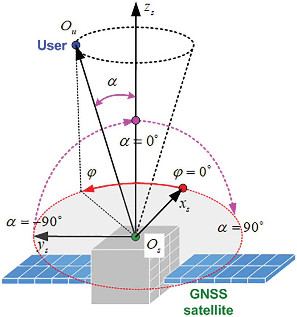
Figure 2. Schematic diagram of the transmitting antenna
The coverage area of the GNSS signal in a certain axial section of the boresight-axis is shown in Figure 3.
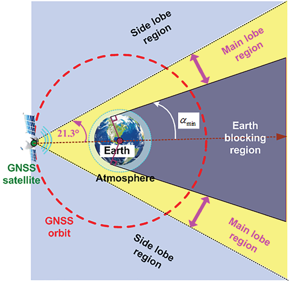
Figure 3. Schematic diagram of GNSS signal coverage areas
Under the influence of Earth blocking, the minimum absolute value of the beam angle of the GNSS signal reaching high-altitude space is:
 \begin{equation}{\alpha _{\min }} = \arcsin \left( {\frac{{{R_\textrm{e}}}}{{{R_{\text{GNSS}}}}}} \right) = \textrm{13}.\textrm{9}^\circ \end{equation}
where  ${R_\textrm{e}}$=6378 km is the Earth's radius and
  ${R_{\text{GNSS}}}$ represents the geocentric distance of the GNSS satellite;
  ${R_{\text{GNSS}}}$ = 26,560 km for GPS.
Since the main lobe beam range is  $|\alpha |\lt 21.3^\circ $ (ICD-GPS, 2019), the beam angle range of the main lobe signal reaching high-altitude space is:
 \begin{equation}{\alpha _{\min }} \lt |\alpha |\lt 21.3^\circ\end{equation}
The proportion of main lobe signal reaching high-altitude space to the total main lobe signal is just 34.7%:
 \begin{equation}{\eta _{\text{main}}} = \left( {1 - \frac{{13.9^\circ }}{{21.3^\circ }}} \right) \times 100\%= 34.7\%\end{equation}
The remaining 65⋅3% of the main lobe signal is blocked by the Earth and cannot reach high-altitude space. Reaching the user's location is one of the conditions for a GNSS signal to be visible, so the narrow coverage of main lobe signal in high-altitude space will have a negative impact on the signal's visibility.
The side lobe beam range is  $21.3^\circ \lt |\alpha |\lt 90^\circ $, accounting for
 \begin{equation}{\eta _{\text{side}}} = \left( {1 - \frac{{21.3^\circ }}{{90^\circ }}} \right) \times 100\%= 76.3\%\end{equation}
of the total beam range of the GNSS signal. Unlike the main lobe signal, the side lobe signal cannot be blocked by the Earth, so the combination of main lobe signal and side lobe signal can improve the visibility of GNSS signal in high-altitude space.
3.2. GNSS signal strength characteristics
The signal transmitter, the transmission path, and the receiving terminal together form the signal transmission link, as shown in Figure 4. The following sub-sections focus on the influence of transmitting antenna gain and signal transmission loss on the strength characteristics of the GNSS signal. Based on this, the quantitative study of the distribution characteristics of signal received power is performed.
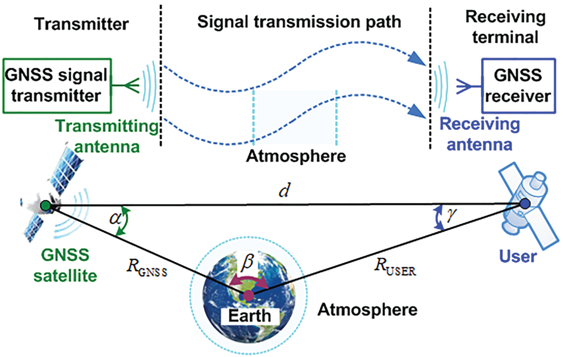
Figure 4. Schematic of GNSS signal transmission link in high-altitude space
3.2.1. Transmitting antenna gain
The directivity of the transmitting antenna gain directly affects the signal strength of different transmission directions. The following describes the directivity of the transmitting antenna gain according to the test results of the GPS Block IIR-M satellite (Marquis and Reigh, Reference Marquis and Reigh2015). The test results (L1 signal) of the GPS satellite with the space vehicle number (SVN) set at 50 are shown in Figure 5.

Figure 5. Results of transmitting antenna gain. (The test results of different azimuths are distinguished by scatter points of different colours, and the fitting results are indicated by solid red line.)
Figure 5 indicates that the gain of the transmitting antenna in the main beam range is more than 5 dB, and the gain of the transmitting antenna within the Earth coverage area is more than 14 dB; while in the side beam range, the gain decreases rapidly with the increase of the absolute value of beam angle, most of which is below 0 dB, and the worst is −50 dB. In addition, the transmitting antenna gains in the range of the main lobe beam have good consistency at different azimuths, while the gains in the range of the side lobe beam show strong fluctuations with the change of azimuth. However, from the overall test results, the transmitting antenna gain is mainly affected by the beam angle.
In order to focus on the influence of beam angle on the signal’s strength characteristics, the test results of different azimuths are averaged, and the fitting results of the transmission antenna gain with the change of beam angle are obtained by cubic spline interpolation. The fitting results in Figure 5 are consistent with the trend of the gain changing with the beam angle in the test results. In general, the gain of the transmitting antenna in the range of the side lobe beam is significantly lower than that in the range of main lobe beam, which will have a negative impact on the utilisation of side lobe signal by high-altitude users.
3.2.2. Signal transmission loss
The calculation equation of signal transmission loss  ${L_d}$ is:
 \begin{equation}{L_d} = 20\lg \left( {\frac{\lambda }{{4\pi d}}} \right)\end{equation}
where  $\lambda$ is the carrier wavelength,
  $\lambda$=0⋅19 m for GPS L1 carrier, and d is the signal transmission distance.
The relationship between the signal transmission distance d, the beam angle  $\alpha$ and the user's geocentric distance
  ${R_{\text{USER}}}$ is analysed below. In a certain axial section of the boresight-axis, the geometric relationship between the user, the GNSS satellite and the Earth is established as shown in Figure 6.

Figure 6. Geometric relationship between the user, the GNSS satellite and the Earth
In Figure 6, the Earth centre plane frame ( ${O_e} - {x_e}{y_e}$ frame, abbreviated as
  $e$-frame) can be established. In the triangle formed by the user, the GNSS satellite and the Earth's centre, it can be obtained according to the sine and cosine theorems:
 \begin{align}\frac{{\sin (\alpha )}}{{{R_{\text{USER}}}}} &= \frac{{\sin (\gamma )}}{{{R_{\text{GNSS}}}}} = \frac{{\textrm{sin}(\beta )}}{d}\end{align}
 \begin{align}\gamma &= \arccos \left( {\frac{{R_{\text{USER}}^2 + {d^2} - R_{\text{GNSS}}^2}}{{2{R_{\text{USER}}}d}}} \right)\end{align}
 \begin{align}d &= \sqrt {R_{\text{GNSS}}^2 + R_{\text{USER}}^2 - 2{R_{\text{GNSS}}}{R_{\text{USER}}}\cos (\beta )}\notag\\ &= \sqrt {R_{\text{GNSS}}^2 + R_{\text{USER}}^2 + 2{R_{\text{GNSS}}}{R_{\text{USER}}}\cos ({\alpha + \gamma } )}\end{align}
where  $\beta$ represents the angle of the user and the GNSS satellite relative to the Earth's centre, and
  $\gamma$ represents the Earth's centre and the GNSS satellite relative to the user.
For the high-altitude user,  ${R_{\text{USER}}} \gt {R_{\text{GNSS}}}$, so Equation (3.7) indicates that
  $\gamma \lt 90^\circ $. Further combining with Equation (3.6), we obtain:
 \begin{equation}\gamma = \arcsin \left[ {\frac{{{R_{\text{GNSS}}}}}{{{R_{\text{USER}}}}}\sin (\alpha )} \right]\end{equation}
By substituting Equation (3.9) into Equation (3.8), we obtain:
 \begin{equation}d = \sqrt {R_{\text{GNSS}}^2 + R_{\text{USER}}^2 + 2{R_{\text{GNSS}}}{R_{\text{USER}}}\cos \left\{ {\alpha + \arcsin \left[ {\frac{{{R_{\text{GNSS}}}}}{{{R_{\text{USER}}}}}\sin (\alpha )} \right]} \right\}}\end{equation}
 Equation (3.10) indicates that when the geocentric distance  ${R_{\text{USER}}}$ is constant, the transmission distance d decreases with an increasing beam angle
  $\alpha$. Therefore, when reaching high-altitude space with the same geocentric distance, the transmission distance of the main lobe signal is greater than that of the side lobe signal.
The spatial distribution of GNSS signal transmission loss is analysed. The plane of the  $e$-frame is divided into 10 km × 10 km grids, and the results shown in Figure 7 are obtained after traversing all grid points.

Figure 7. Spatial distribution of GNSS signal transmission loss
Figure 7 shows that the transmission loss of the GNSS signal reaching high-altitude space is increased by the influence of the increase of the signal transmission distance. At the same orbital height in high-altitude space, the transmission distance of the main lobe signal is greater than that of the side lobe signal, so the transmission loss of the main lobe signal is greater than that of the side lobe signal. Obviously, the large signal transmission loss has an adverse impact on the utilisation of GNSS signal by high-altitude users.
3.2.3. Power of signal received
The power of the GNSS signal received can be expressed as:
 \begin{equation}{P_R} = {P_T} + {G_T} + {L_d} + {G_R}\end{equation}
where  ${P_T}$ is the signal transmitted power,
  ${P_T}$ = 14⋅28 dBW for GPS (ICD-GPS, 2019),
  ${G_T}$ is the transmitting antenna gain, and
  ${G_R}$ is the receiving antenna gain. In practical applications, the gain of the receiving antenna is usually designed according to different mission requirements. Here we focus on analysing the strength distribution characteristics of GNSS signal in high-altitude space, so, without loss of generality, it is assumed that the receiving antenna is an omnidirectional antenna with a gain of 0 dB.
First, the beam angle  $\alpha$ and signal propagation distance d are calculated according to the position coordinates of each grid point and GNSS satellite in
  $e$-frame. Second, according to the fitting results in Figure 5, the transmitting antenna gain corresponding to the beam angle
  $\alpha$ can be obtained. Then, the signal propagation loss
  ${L_d}$ can be calculated by substituting the signal propagation distance d into Equation (3.5). Finally, the power of the signal received can be obtained by substituting the transmitting antenna gain
  ${G_T}$, signal transmission loss
  ${L_d}$, signal transmitted power
  ${P_T}$=14⋅28 dBW and the receiving antenna gain
  ${G_R}$=0 dB input Equation (3.11). The spatial distribution of the power of the signal received is shown in Figure 8.

Figure 8. Spatial distribution of the power of the signal received
Figure 8 shows that the spatial distribution of the power of the GNSS signal received mainly varies with the beam angle and the signal propagation distance. At the same orbital altitude in high-altitude space, although the signal transmission loss decreases with an increasing beam angle, the power of the signal received still decreases rapidly with an increasing beam angle. This reflects the fact that the power of the signal received at the same orbital altitude is mainly affected by the beam angle. That is, the received power of the main lobe signal at the same orbital altitude is higher than that of the side lobe signal. Because the signal strength being higher than the receiver sensitivity is one of the conditions for a GNSS signal to be visible, it is necessary to further improve the receiver sensitivity to improve the visibility of GNSS signals in high-altitude space.
4. Geometric configuration and GDOP of visible GNSS satellites
4.1. Geometric configuration
The geometric configuration of visible GNSS satellites is affected by the geometric relationship of visible satellites to the user. Figure 9 shows the geometric configuration of visible GNSS satellites in high-altitude space.
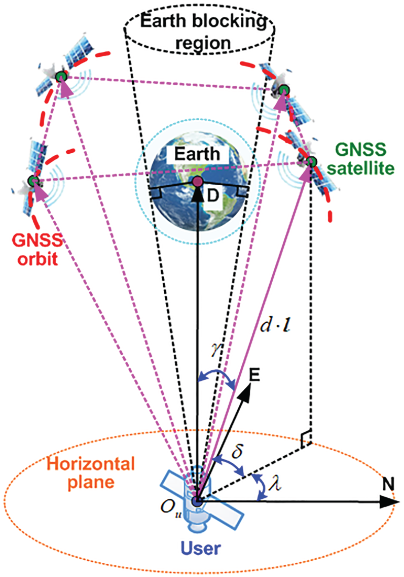
Figure 9. Schematic diagram of the geometric configuration
In the North-East-Down frame (NED-frame), the unit line of sight (LOS) vector of the high-altitude user pointing to a GNSS satellite can be described by the elevation  $\delta$ and the azimuth
  $\lambda$. The larger the distribution range of elevation and azimuth of the visible satellites, that is, the more uniform the distribution of visible satellites, the better the geometric configuration.
The elevation and the beam angle meet the following relationship:
 \begin{equation}\frac{{\cos (\delta )}}{{{R_{\text{GNSS}}}}} = \frac{{\sin (\gamma )}}{{{R_{\text{GNSS}}}}} = \frac{{\sin (\alpha )}}{{{R_{\text{USER}}}}}\end{equation}
From Equation (4.1), we obtain:
 \begin{equation}\delta = \arccos \left[ {\frac{{{R_{\text{GNSS}}}}}{{{R_{\text{USER}}}}}\sin (\alpha )} \right]\end{equation}
Equation (4.2) indicates that the elevation distribution range is related to the beam angle range of the received GNSS signals.
When the maximum beam angle of the GNSS signals that the high-altitude user can receive is  ${\alpha _{\max }}$, according to Equation (4.2), the minimum elevation of the visible GNSS satellites can be obtained as:
 \begin{equation}{\delta _{\min }} = \arccos \left[ {\frac{{{R_{\text{GNSS}}}}}{{{R_{\text{USER}}}}}\sin ({\alpha_{\max }})} \right]\end{equation}
Besides, under the influence of Earth blocking, the maximum elevation of visible GNSS satellites is:
 \begin{equation}{\delta _{\max }} = \arccos \left[ {\frac{{{R_\textrm{e}}}}{{{R_{\text{USER}}}}}} \right]\end{equation}
Combining Equations (4.3) and (4.4), the elevation distribution range of visible GNSS satellites for the high-altitude user is:
 \begin{equation}\arccos \left[ {\frac{{{R_{\text{GNSS}}}}}{{{R_{\text{USER}}}}}\sin ({\alpha_{\max }})} \right] \lt \delta \lt \arccos \left[ {\frac{{{R_\textrm{e}}}}{{{R_{\text{USER}}}}}} \right]\end{equation}
Taking GPS as an example, the result calculated according to Equation (4.5) is shown in Figure 10. Figure 10 indicates that both the maximum and minimum elevations of visible GNSS satellites increase with an increasing geocentric distance of the high-altitude user, and the elevation distribution range decreases with an increasing geocentric distance of the high-altitude user. When the geocentric distance of the high-altitude user is constant, the minimum elevation of visible GNSS satellites increases as the maximum beam angle decreases, and the elevation distribution range decreases accordingly.

Figure 10. Elevation distribution range in high-altitude space
4.2. GDOP
The positioning errors and the pseudorange errors of visible GNSS satellites meet:
 \begin{equation}\left[ {\begin{array}{* {20}{c}} {\Delta {\rho^{(1)}}}\\ {\Delta {\rho^{(2)}}}\\ {\ldots }\\ {\Delta {\rho^{(N)}}} \end{array}} \right] = \left[ {\begin{array}{* {20}{c}} {l_x^{(1)}}&{l_y^{(1)}}&{l_z^{(1)}}&{ - 1}\\ {l_x^{(2)}}&{l_y^{(2)}}&{l_z^{(2)}}&{ - 1}\\ {\ldots }&{\ldots }&{\ldots }&{\ldots }\\ {l_x^{(N)}}&{l_y^{(N)}}&{l_z^{(N)}}&{ - 1} \end{array}} \right]\left[ {\begin{array}{* {20}{c}} {\Delta x}\\ {\Delta y}\\ {\Delta z}\\ {\Delta \delta {t_u}} \end{array}} \right]\end{equation}
where  ${[\begin{array}{* {20}{c}} {\Delta x}&{\Delta y}&{\Delta z} \end{array}]^\textrm{T}}$ is the user's position error,
  $\Delta \delta {t_u}$ is the error of the receiver clock bias;
  $\Delta {\rho ^{(j)}}$ is the pseudorange error of the jth visible satellite,
  $j = 1,2,\ldots ,N$ and
  $N \ge 4$;
  $l_x^{(j)}$,
  $l_y^{(j)}$ and
  $l_z^{(j)}$ represent the three components of the unit LOS vector
  ${{\boldsymbol l}^{(j)}}$ in the NED-frame, respectively.
Note that  $\Delta {\boldsymbol X} = {\left[ {\begin{array}{*{20}{c}} {\Delta x}&{\Delta y}&{\Delta z}&{\Delta \delta {t_u}} \end{array}} \right]^\textrm{T}}$and
  $\Delta {\boldsymbol Z} = {[\begin{array}{*{20}{c}} {\Delta {\rho ^{(1)}}}&{\Delta {\rho ^{(2)}}}&{\ldots }&{\Delta {\rho ^{(N)}}} \end{array}]^\textrm{T}}$, then Equation (4.6) can be written as:
 \begin{equation}\Delta \boldsymbol{Z} = \boldsymbol{H}\Delta \boldsymbol{X},\;\boldsymbol{H} = \left[ {\begin{array}{* {20}{c}} {l_x^{(1)}}&{l_y^{(1)}}&{l_z^{(1)}}&{ - 1}\\ {l_x^{(2)}}&{l_y^{(2)}}&{l_z^{(2)}}&{ - 1}\\ {\ldots }&{\ldots }&{\ldots }&{\ldots }\\ {l_x^{(N)}}&{l_y^{(N)}}&{l_z^{(N)}}&{ - 1} \end{array}} \right], \end{equation}
The magnification of the total positioning and timing error to the pseudorange error is defined as the GDOP, and its calculation formula is as follows:
 \begin{equation}{K_{GDOP}} = \sqrt {\textrm{tr[}{{({{\boldsymbol H}^\textrm{T}}{\boldsymbol H})}^{ - 1}}\textrm{]}}\end{equation}
 Let  ${\boldsymbol G} = {({{\boldsymbol H}^\textrm{T}}{\boldsymbol H})^{ - 1}}$, and expand
  ${\boldsymbol G}$ to obtain (Chaffee and Abel, Reference Chaffee and Abel1994):
 \begin{equation}\boldsymbol{G} = \left[ {\begin{array}{* {20}{c}} \boldsymbol{\varGamma }&{\boldsymbol{\varGamma {\bar l}}}\\ {{{\bar{\boldsymbol{l}}}^\textrm{T}}\boldsymbol{\varGamma }}&{\dfrac{\textrm{1}}{N}({\textrm{1} + {{\bar{\boldsymbol{l}}}^\textrm{T}}\boldsymbol{\varGamma {\bar l}}} )} \end{array}} \right],\;\bar{\boldsymbol{l}} = \frac{\textrm{1}}{N}\sum\limits_{\text{j} = \textrm{1}}^\textrm{N} {{\boldsymbol{l}^{(j)}}} ,\;{\boldsymbol{\varGamma }^{ - 1}} = \sum\limits_{\text{j} = \textrm{1}}^\textrm{N} {[{{\boldsymbol{l}^{(j)}} - \bar{\boldsymbol{l}}} ]} {[{{\boldsymbol{l}^{(j)}} - \bar{\boldsymbol{l}}} ]^\textrm{T}}\end{equation}
where  $\bar{\boldsymbol{l}}$ and
  ${{\boldsymbol \varGamma }^{ - 1}}$ represent the mean and covariance of the unit LOS vectors, respectively. According to Equation (4.9),
  ${K_{GDOP}}$ can be obtained as:
 \begin{equation}{K_{GDOP}} = \sqrt {\textrm{tr(}{\boldsymbol G})} = \sqrt {\textrm{tr(}{\boldsymbol \varGamma }) + \frac{\textrm{1}}{N}({\textrm{1} + {{\bar{\boldsymbol{l}}}^\textrm{T}}{\boldsymbol \varGamma {\bar l}}} )}\end{equation}
 Equation (4.10) indicates that the number of visible satellites, and the mean and covariance of the unit LOS vectors all affect the GDOP. Covariance  ${{\boldsymbol \varGamma }^{ - 1}}$ is related to the distribution uniformity of visible GNSS satellites. The better the distribution uniformity of visible GNSS satellites is, the smaller
  $\textrm{tr(}{\boldsymbol \varGamma })$ is. Because the distribution uniformity of the visible GNSS satellites reflects the pros and cons of the geometric configuration, the greater the number of visible GNSS satellites and the better the geometric configuration, the smaller the value of the GDOP.
5. Dynamic performance and Doppler shift range
The Doppler shift range of GNSS signals received by the high-altitude user is analysed below. Figure 11 shows the relative motion of the high-altitude user and the GNSS satellite.

Figure 11. Schematic diagram of the dynamic performance of the high-altitude user
The Doppler shift  ${f_D}$ can be expressed as:
 \begin{equation}{f_D} = - \frac{{{f_s}}}{c}\frac{{{{({{{\boldsymbol v}_u} - {{\boldsymbol v}_s}} )}^\textrm{T}}({{{\boldsymbol r}_u} - {{\boldsymbol r}_s}} )}}{{|{{{\boldsymbol r}_u} - {{\boldsymbol r}_s}} |}}\end{equation}
where  ${{\boldsymbol r}_u}$ and
  ${{\boldsymbol r}_s}$ represent the position of the user and GNSS satellite, respectively;
 ${{\boldsymbol v}_u}$ and
  ${{\boldsymbol v}_s}$ represent the velocity of the user and GNSS satellite, respectively;
  ${f_s}$ represents the signal transmitted frequency,
  ${f_s}$=1575⋅42 MHz for GPS L1 signal; c represents the speed of light.
Since the GNSS satellite is in a circular (or near circular) orbit, we obtain:
 \begin{equation}{{\boldsymbol v}_s} = \frac{{{{\boldsymbol h}_s} \times {{\boldsymbol r}_s}}}{{R_{\text{GNSS}}^2}}\end{equation}
where  ${{\boldsymbol h}_s}$ is the angular momentum of the GNSS satellite, and
  ${{\boldsymbol h}_s}$ is expressed in the geocentric equatorial inertial frame (abbreviated as
  $i$-frame) as:
 \begin{equation}{\boldsymbol h}_s^i = \sqrt {\mu {R_{\text{GNSS}}}} {\left[ {\begin{array}{* {20}{c}} {\sin ({{i_s}} )\cos ({{\Omega_s}} )}&{ - \sin ({{i_s}} )\sin ({{\Omega_s}} )}&{\cos ({{i_s}} )} \end{array}} \right]^\textrm{T}}\end{equation}
where  ${i_s}$ and
  ${\Omega_s}$ are the inclination and the right ascension of ascending node (RAAN) of the GNSS satellite's orbit, respectively.
  $\mu = 3.896 \times {10^{14}}$is the gravitational constant of the Earth.
When the user's orbit is also a circular orbit, the same can be obtained:
 \begin{equation}{{\boldsymbol v}_u} = \frac{{{{\boldsymbol h}_u} \times {{\boldsymbol r}_u}}}{{R_{\text{USER}}^2}}\end{equation}
where  ${{\boldsymbol h}_u}$ is the angular momentum of the user, and
  ${{\boldsymbol h}_u}$ is expressed in the
  $i$-frame as:
 \begin{equation}{\boldsymbol h}_u^i = \sqrt {\mu {R_{\text{USER}}}} {\left[ {\begin{array}{* {20}{c}} {\sin ({{i_u}} )\cos ({{\Omega_u}} )}&{ - \sin ({{i_u}} )\sin ({{\Omega_u}} )}&{\cos ({{i_u}} )} \end{array}} \right]^\textrm{T}}\end{equation}
where  ${i_u}$ and
  ${\Omega_u}$ are the inclination and the RAAN of the user's orbit, respectively.
Substituting Equations (5.2) and (5.4) into Equation (5.1), we obtain:
 \begin{align} {f_D} & =- \dfrac{{{f_s}}}{c}{\left( {\dfrac{{{\boldsymbol{h}_u} \times {\boldsymbol{r}_u}}}{{R_{\text{USER}}^2}} - \dfrac{{{\boldsymbol{h}_s} \times {\boldsymbol{r}_s}}}{{R_{\text{GNSS}}^2}}} \right)^\textrm{T}}\dfrac{{({{\boldsymbol{r}_u} - {\boldsymbol{r}_s}} )}}{{|{{\boldsymbol{r}_u} - {\boldsymbol{r}_s}} |}} = \dfrac{{{f_s}}}{c}{\left( {\dfrac{{{\boldsymbol{h}_u}}}{{R_{\text{USER}}^2}} - \dfrac{{{\boldsymbol{h}_s}}}{{R_{\text{GNSS}}^2}}} \right)^\textrm{T}}\dfrac{{({{\boldsymbol{r}_u} \times {\boldsymbol{r}_s}} )}}{{|{{\boldsymbol{r}_u} - {\boldsymbol{r}_s}} |}}\notag\\ & =\dfrac{{{f_s}}}{c}\boldsymbol{H}_{s,u}^\textrm{T}{\boldsymbol{R}_{s,u}} = \dfrac{{{f_s}}}{c}{h_{s,u}}{r_{s,u}}\cos (\theta )\end{align}
 \begin{align}{\boldsymbol{H}_{s,u}} &= \frac{{{\boldsymbol{h}_u}}}{{R_{\text{USER}}^2}} - \frac{{{\boldsymbol{h}_s}}}{{R_{\text{GNSS}}^2}},\;{\boldsymbol{R}_{s,u}} = \frac{{{\boldsymbol{r}_u} \times {\boldsymbol{r}_s}}}{{|{{\boldsymbol{r}_u} - {\boldsymbol{r}_s}} |}}\end{align}
where  $\theta$ is the angle between
  ${{\boldsymbol H}_{s,u}}$ and
  ${{\boldsymbol R}_{s,u}}$,
  ${h_{s,u}}$ and
  ${r_{s,u}}$ are the magnitude of
  ${{\boldsymbol H}_{s,u}}$ and
  ${{\boldsymbol R}_{s,u}}$, respectively.
First,  ${h_{s,u}}$ can be expressed as:
 \begin{equation}{h_{s,u}} = |{{{\boldsymbol H}_{s,u}}} |= \sqrt {\frac{{{{|{{{\boldsymbol h}_u}} |}^2}}}{{R_{\text{USER}}^4}} + \frac{{{{|{{{\boldsymbol h}_s}} |}^2}}}{{R_{\text{GNSS}}^4}} - 2\frac{{{\boldsymbol h}_u^\textrm{T}{{\boldsymbol h}_s}}}{{R_{\text{USER}}^2R_{\text{GNSS}}^2}}}\end{equation}
Substituting Equations (5.3) and (5.5) into Equation (5.8), we obtain:
 \begin{align}{h_{s,u}} &= \sqrt {\frac{\mu }{{R_{\text{USER}}^3}} + \frac{\mu }{{R_{\text{GNSS}}^3}} - 2\mu \frac{{f({{i_s},{\Omega_s},{i_u},{\Omega_u}} )}}{{\sqrt {R_{\text{USER}}^3R_{\text{GNSS}}^3} }}}\end{align}
 \begin{align} f({{i_s},{\Omega_s},{i_u},{\Omega_u}} )& =\sin ({{i_s}} )\cos ({{\Omega_s}} )\sin ({{i_u}} )\cos ({{\Omega_u}} )\notag\\ & \quad + \sin ({{i_s}} )\sin ({{\Omega_s}} )\sin ({{i_u}} )\sin ({{\Omega_u}} )+ \cos ({{i_s}} )\cos ({{i_u}} )\end{align}
 Obviously,  ${h_{s,u}}$ is a constant for the specific user.
Second,  ${r_{s,u}}$ can be expressed as:
 \begin{equation}{r_{s,u}} = |{{{\boldsymbol R}_{s,u}}} |= \frac{{|{{{\boldsymbol r}_u} \times {{\boldsymbol r}_s}} |}}{{|{{{\boldsymbol r}_u} - {{\boldsymbol r}_s}} |}} = {R_{\text{USER}}}{R_{\text{GNSS}}}\frac{{\sin (\beta )}}{d}\end{equation}
Simultaneously Equations (3.6), (4.1) and (5.11), we obtain:
 \begin{equation}{r_{s,u}} = {R_{\text{USER}}}{R_{\text{GNSS}}}\frac{{\sin (\gamma )}}{{{R_{\text{GNSS}}}}} = {R_{\text{USER}}}\sin (\gamma ) = {R_{\text{USER}}}\cos (\delta )\end{equation}
 Equation (5.12) indicates that  ${r_{s,u}}$ decreases with the increase of elevation.
Finally, the angular momentums  ${{\boldsymbol h}_u}$ and
  ${{\boldsymbol h}_s}$ are both constant vectors, so
  ${{\boldsymbol H}_{s,u}}$ is also a constant vector. The direction of
  ${{\boldsymbol R}_{s,u}}$ changes with the position of the user and the GNSS satellite, so when
  ${{\boldsymbol R}_{s,u}}$ and
  ${{\boldsymbol H}_{s,u}}$ are in the same direction, the Doppler shift reaches the maximum value
 \begin{equation}{f_{D,\max }}(\delta )= \frac{{{f_s}}}{c}|{{{\boldsymbol H}_{s,u}}} ||{{{\boldsymbol R}_{s,u}}} |= \frac{{{f_s}}}{c}{h_{s,u}}{r_{s,u}} = \frac{{{f_s}}}{c}{h_{s,u}}{R_{\text{USER}}}\cos (\delta )\end{equation}
of the corresponding elevation. Similarly, when  ${{\boldsymbol R}_{s,u}}$ and
  ${{\boldsymbol H}_{s,u}}$ are in the opposite direction, the Doppler shift reaches the minimum value
  ${f_{D,\textrm{min}}}(\delta )= - {f_{D,\textrm{max}}}(\delta )$ of the corresponding elevation.
The GEO user fixed at (105⋅6° E, 0° N) is analysed as an example. The Doppler shift of GPS L1 signal received by the GEO user in different elevations in one orbital period is shown in Figure 12.

Figure 12. Doppler shift in different elevations. (Solid lines of different colours are used to distinguish different visible GPS satellites.)
Figure 12 shows that the Doppler shift range decreases as the elevation increases. Moreover, the Doppler shift results are all within the theoretical range obtained by Equation (5.13). Therefore, the functional relationship between the Doppler shift range and the elevation can be used to determine the Doppler search range of the GNSS signal acquisition.
6. Simulation evaluation of availability of GNSS signals in high-altitude space
6.1. GNSS constellations simulation platform
Taking J2000⋅0 Earth Centred Inertial and Coordinated Universal Time (UTC) as the space and time reference respectively, the GNSS constellations simulation platform including GPS and BDS is built according to the state of each GNSS when the constellations are fully deployed. The main orbital parameters are shown in Table 1 (ICD-BDS, 2019; ICD-GPS, 2019).
Table 1. Orbital parameters of GNSS constellations

6.2. Simulation results and analysis
The GEO optical remote sensing satellite GaoFen-4 (GF-4), which was launched by China and is fixed at (105⋅6° E, 0° N), was used as the application object (Zheng et al., Reference Zheng, Liu, Yang and Li2019). The simulation duration is set as one orbital period, and the simulation interval is 1 s.
6.2.1. Signal received power
First, regardless of the limitation of receiver sensitivity, all GNSS signals that reach the location of GF-4 are considered visible. The statistical results of signal received power are shown in Figure 13, and the signal received power of the GPS satellite with SVN set at 50 over time is shown in Figure 14.

Figure 13. Statistical results of signal received power

Figure 14. Power of signal received over time
The results in Figures 13 and 14 show that the power of the signal received is mainly concentrated between −190 and −180 dBW, accounting for 82% of the total received signal. Since the high-altitude user needs to utilise the main and side lobe signals simultaneously, with large differences in received power, the GNSS receivers need to be designed from the following aspects:
1. The acquisition of weak signals will be seriously hindered by cross-correlation, which can easily cause the phenomenon of false acquisition or acquisition failure. Therefore, the GNSS receiver should improve the anti-correlation interference performance of the acquisition algorithm.
2. Since the high-altitude user can still receive the main lobe signals, the tracking loop in the GNSS receiver can adopt a vector tracking structure to realise the assistance of strong signals to weak signals through channel coupling and information sharing.
3. Since there is a large difference between the measurement errors corresponding to strong and weak signals, the GNSS receivers need to estimate the variance of the measurement error corresponding to each signal based on the received power, and to further improve the navigation accuracy through the weighted processing.
In addition, the transmitting antenna gains in the range of the side lobe beam show strong fluctuations with the change of azimuth, so the received power of side lobe signals has strong instantaneous fluctuations. When the received power of side lobe signals fluctuates at levels near the limits of sensitivity of the GNSS receiver, the difficulty of signals locking will be increased or the locked signals will be lost, thus reducing the signal availability.
The results for the power of GPS signal received in different elevations for GF-4 are shown in Figure 15. Figure 15 shows that the visible GPS satellites for GF-4 are concentrated in the high-elevation range of 50°–80°, and the power of the signal received decreases as the elevation decreases, so the receiving antenna gain can be designed accordingly. It is necessary to focus on the gain in the elevation range of 50°–80°, and the gain in the elevation range of 50°–70° can be increased appropriately. For high-altitude users, the beam angle of the received signal changes with the elevation, and the beam angle directly affects the transmit antenna gain, signal propagation distance and loss. Therefore, unlike ground users, the power of signals received by high-altitude users will change significantly with the elevation. In addition, the high-altitude user can adopt multi-antenna non-coplanar installation mode to achieve attitude determination. In this way, not only can mutual blocking between the antennas be avoided, but also the combinations of main antenna and slave antennas can be better utilised, thereby improving the accuracy of attitude determination.

Figure 15. Power of signal received in different elevations
6.2.2. Doppler shift and Doppler rate
The Doppler shift and Doppler rate of the GPS L1 signal received by GF-4 over time are shown in Figures 16 and 17, respectively. The Doppler search range of ordinary GNSS receivers used by ground users is ±5 kHz, while the Doppler search range required by GF-4 is ±15 kHz. This requirement is equivalent to that of high dynamic GNSS receivers used by ground users. The wide range of Doppler shift and Doppler rate will bring some difficulties to the acquisition and tracking of GNSS signals. Therefore, high-altitude users can predict both Doppler shift and Doppler rate by using their own orbit parameter information or combined with the navigation solution of an orbital filter (Capuano et al., Reference Capuano, Basile, Botteron and Farine2016b, Reference Capuano, Blunt, Botteron and Farine2017b). In addition, when a high-altitude spacecraft performs a manoeuvre to change its orbit, the accelerometers can sense non-gravitational acceleration. Therefore, under this condition, the accelerometers can be used to narrow the uncertainty range of Doppler shift and Doppler rate.

Figure 16. Doppler shift over time

Figure 17. Doppler rate over time
6.2.3. Number of visible satellites and GDOP
Combined with different receiver sensitivity conditions, the number of visible GNSS satellites and GDOP in four different constellation combinations is analysed. The statistical results of the ratio of the time when the number of visible satellites exceeds the threshold to the entire orbital period and the mean of GDOP are shown in Figures 18 and 19, respectively. Combining Figures 18 and 19 shows that for the same constellation combination, the higher the receiver sensitivity, the more visible satellites and the better geometric configuration, so the mean of GDOP is smaller. Under the same receiver sensitivity condition, the more GNSS constellations involved in the combination, the more visible satellites and the better geometric configuration, so the mean of GDOP is smaller. Besides medium Earth orbit (MEO), GEO and inclined geosynchronous orbit (IGSO) are also included in the orbit types of BDS, which is the main reason for the differences between the results of different constellation combinations.

Figure 18. Statistical results of the number of visible satellites

Figure 19. Statistical results of GDOP
7. Conclusion
After a comprehensive and systematic analysis of the availability of GNSS signals in high-altitude space, the following conclusions can be obtained:
Due to the influence of Earth blocking, the proportion of the GNSS main lobe signal reaching high-altitude space to the total main lobe signal is just 34⋅7%. However, the side lobe signal, which accounts for 76⋅3% of the total beam range of the GNSS signal, is not blocked by the Earth. Therefore, the combination of main lobe signals and side lobe signals can improve the visibility of GNSS signals in high-altitude space.
The spatial distribution characteristics of the GNSS signal received power are mainly related to the transmitting antenna gain and the signal transmission loss. Since the transmission distance of GNSS signals in high-altitude space is long, and most of the GNSS signal reaching high-altitude space is side lobe signal, the transmission loss of GNSS signals is large and the transmitting antenna gain is generally reduced. Because of these two factors, the received power of GNSS signals in high-altitude space is generally low.
Since the power of the main lobe signals and the side lobe signals received are quite different, the acquisition of weak signals by the GNSS receiver will be affected by the cross-correlation interference of strong signals. Therefore, in addition to considering the influence of noise on the performance of weak signals acquisition, the GNSS receivers equipped by high-altitude users also need to improve the anti-correlation interference performance of the acquisition algorithm.
The GNSS satellites visible to the high-altitude user are concentrated in the high-elevation range, and the power of the signal received decreases as the elevation decreases. Therefore, it is necessary to focus on the gain in the high-elevation range, and the gain in the elevation range corresponding to the side lobe signal can be increased appropriately.
The strong dynamic performance of high-altitude users makes the range of Doppler shift and Doppler rate of the received GNSS signals large, thereby reducing the acquisition speed and the stability of the tracking loop. When a high-altitude spacecraft performs a manoeuvre to change its orbit, the accelerometers can be used to narrow the uncertainty range of the Doppler shift and Doppler rate; otherwise, the high-altitude spacecraft can predict Doppler shift and Doppler rate by using its own orbit parameter information or combined with the navigation solution of an orbital filter.
In general, due to the influence of Earth blocking, the coverage area of the main lobe signals in high-altitude space is narrow. The coverage area of side lobe signals in high-altitude space is large, but the power of the side lobe signals received is significantly lower than that of the main lobe signals at the same orbital altitude. In addition, influenced by the increased distance of signal transmission, the transmission loss of GNSS signals reaching high-altitude space increases further. Therefore, the major difficulty faced by GNSS-based high-altitude applications is the generally weak GNSS signals. The use of a high-sensitivity GNSS receiver with multi-constellation compatibility can improve the visibility of signals and the geometric configuration of visible satellites, which has positive significance for the availability of GNSS signals in high-altitude space. Our analysis is based on the general characteristics of high-altitude space above the GNSS constellation. Therefore, the conclusions of our research have universal application value for spacecraft above the GNSS constellation.
Acknowledgments
This work was supported by the Natural Science Foundation of China (NSFC) (grant number 61673040 and 61074157), the Joint Projects of NSFC-CNRS (grant number 61111130198), the Aeronautical Science Foundation of China (grant number 2015ZC51038 and 20170151002) and the Project of the Experimentation and Technology Research (1700050405). The work is also supported by the Open Research Fund of State Key Laboratory of Space-Ground Integrated Information Technology under grant number 2015-SGIIT-KFJJ-DH-01.


