1. INTRODUCTION
The presence of the US GPS and the Russian GLONASS, and the upcoming constellations of a number of the new global and regional augmentation navigation satellite systems (the European Galileo, the Chinese Compass, the Japanese QZSS and the Indian GAGAN or IRNSS) will introduce additional end-user accuracy everywhere and improve service availability in environments where satellite visibility is often obscured (Gibbons, Reference Gibbons2009). Meanwhile, multiple constellations broadcasting more signals in the same frequency bands will cause interference effects among the systems, making interoperability and compatibility more tedious (Hein, Reference Hein, Avila-Rodriguez, Wallner, Eissfeller, Pany and Hartl2007a, Hein, Reference Hein, Avila-Rodriguez, Wallner, Eissfeller, Pany and Hartl2007b).
Interoperability refers to the ability of global and regional navigation satellite systems and augmentations, and the services they provide, to be used together to provide better capabilities at the user level than would be achieved by relying solely on the open signals of one system. Compatibility refers to the ability of global and regional navigation satellite systems, and augmentations, to be used separately or together without causing unacceptable interference and/or other harm to an individual system and/or service. In order to make open signals and services interoperable and maximize benefit to all global navigation satellite systems (GNSS) users, all GNSS signals and services must be compatible (Hein, Reference Hein2006).
In April 2007, China launched the first middle-Earth orbit (MEO) satellite for Compass, which the nation plans to turn into a fully fledged GNSS system within a few years (XinhuaNews, 2007). In April 2009, a second Compass satellite – this one a geostationary satellite – was launched, which marks the return of China to its GNSS launch program two years after the initial venture into space. The country will complete a 30+ satellite Compass constellation by 2015 (XinhuaNews, 2009). Since Compass uses signal structures similar to other GNSS systems and shares frequencies close to or overlapping those of Galileo, the Galileo and Compass signal overlay becomes a matter of great concern for the system providers and user communities. This issue remains unresolved after two meetings between Chinese and European Union (EU) representatives. This paper mainly deals with the interference computation and simulation among the above-mentioned systems and displays some important analysis results.
Some methodologies for GNSS radio frequency compatibility analyses have been developed in order to assess the intrasystem (interference from the same system) and intersystem (interference from other systems) interference (Titus, Reference Titus, Betz, Hegarty and Owen2003, Wallner, Reference Wallner, Avila-Rodriguez and Hein2006, Wallner, Reference Wallner, Hein, Pany, Avila-Rodriguez and Posfay2005). These methodologies present an extension of the effective carrier power to noise density (C/N 0) theory introduced by John. W. Betz (Betz, Reference Betz2001) to assess the effects of interfering signals in a GNSS receiver. A parameter called spectral separation coefficient (SSC) (Betz, Reference Betz1999) was also introduced to distinguish the effects of interference spectral shape from the effects due to the interfering power. The SSC parameter is an element of the effective C/N 0, which is defined as an inner product of the power spectral densities (PSD) between the desired and interfering signals. In fact, the SSC parameter is appropriate for assessing the impact of interfering signals on the receiver prompt correlator channel processing phases, which are signal acquisition, carrier tracking loop and data demodulation, but not appropriate for the effects on the code tracking loop (DLL) phase. To describe the impact of interfering signals on the code tracking loop phase, a new parameter called code tracking spectral sensitivity coefficient (CT_SSC) was introduced in (Soualle, Reference Soualle and Burger2007a, Soualle, Reference Soualle, Kaindl, Hechenblaikner and Middendorf2007b).
This paper firstly presents an extension of CT_SSC theory in order to assess the effects of intersystem interference on code tracking accuracy. And then a complete methodology combining the SSC and CT_SSC is presented. This method takes into account the space constellation, signal modulation, emission power level, space loss, satellites antenna gain and user receiver characteristic. Computer simulation approach will be adopted in the interference computation for pursuing more realistic results, though it is time consuming to perform the simulation for every interference scenario for different users at every time and place.
Considering the fact that a lot of attention was paid to the signal spectrum overlaps at E1/B1 and E6/B3 band between the above-mentioned systems, intersystem interference will be computed mainly on the two bands where Galileo and Compass signals are sharing the same band. All satellite signals which include (i) the Galileo E1 PRS, E1OS, E6 CS and E6 PRS signals, (ii) the Compass B1, B1-2 and B3 signals, will be taken into consideration in the simulations. In addition, several worse scenarios are simulated, using a 5°×5° grid for latitude and longitude and sampling the period time by a small time steps, i.e. 60 sec.
This paper is organized as follows. Section 1 describes a complete methodology based on SSC and CT_SSC for the interference computation and simulation. Section 2 introduces the constellation and signal parameters used in the computer simulations. Section 3 presents all the simulation and analysis results, while Sections 4 draws conclusions.
METHODOLOGIES
This section provides a detailed derivation of the methodologies used for interference computation and simulation, which is based on the use of different interference coefficients that are calculated for each combination of signals: the spectral separation coefficient and code tracking spectral sensitivity coefficient.
2.1. Formulation
In order to provide a general quantity to reflect the effect of interference on characteristics at the input of a generic receiver, a quantity called effective carrier power to noise density (C/N 0), denoted (C/N 0)eff_SSC, was introduced in (Betz, Reference Betz2001). The (C/N 0)eff_SSC can be interpreted as the carrier power to noise density ratio caused by an equivalent white noise that would yield to the same correlation output variance obtained in presence of interference signal. When intrasystem (interference from the same system) and intersystem (interference from other systems) interference coexists, the (C/N 0)eff_SSC can be expressed as:
where
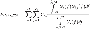
G s(f) is the normalized power spectral density of the desired signal. C is the received power of the useful signal. N 0 is the power spectral density of the thermal noise. In this paper, we assume N 0 to be −201·5 dBW/Hz. G i,j(f) is the normalized spectral density of the j-th interfering signal on the i-th satellite, C i,j the received power of the j-th interfering signal on the i-th satellite, βr the receiver front-end bandwidth, M the visible number of satellites, and K i the number of signals transmitted by satellite i. I GNSS_SSC is the aggregate equivalent noise power density of the combination of intrasystem and intersystem interference.
From (2) it is clear that the impact of the interference on (C/N 0)eff_SSC is directly related to the spectral separation coefficient (SSC) (Betz, Reference Betz1999) of an interfering signal from the j-th interfering signal on the i-th satellite to a desired signal s, the SSC is defined as:
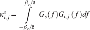
In fact, the SSC parameter is appropriate for assessing the impact of interfering signals on the receiver prompt correlator channel processing phases (acquisition, carrier phase tracking and data demodulation), but not appropriate to evaluate the effects on the DLL phase. For this reason, a new parameter to assess the impact of interfering signals on the code tracking loop phase, called code tracking spectral sensitivity coefficient (CT_SSC) was introduced in (Soualle, Reference Soualle and Burger2007a, Soualle, Reference Soualle, Kaindl, Hechenblaikner and Middendorf2007b). The CT_SSC is defined as:
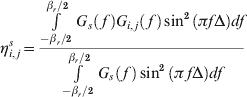
where Δ is the two-sided early-to-late spacing of the correlator.
To provide a metric of similarity to reflect the effect of interfering signals on the code tracking loop phase, a quantity called CT_SSC effective carrier power to noise density (C/N 0), denoted (C/N 0)eff_CT_SSC, is derived in the following text. We recall the method to predict the effect of interference on code tracking accuracy for coherent early-late processing, developed in (Betz, Reference Betz2000a, Betz, Reference Betz and Fine2000b). When there are noise and one non-white interference signal, and the effect of filtering can be neglected within the pass-band, the variance of the code tracking error (in units of seconds squared) can be written as:
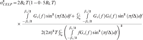
where G l (f) is the normalized spectral density of the interfering signal. C l is the received power of the interfering signal. B L is the one-sided equivalent rectangular bandwidth of the DLL. T is the integration time used in the discriminator. Δ is the two-sided early-late spacing of the correlator.
When there is only white noise, expression (5) can be rewritten as:
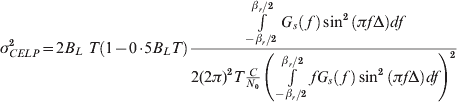
In white noise and nonwhite interference signal, when the variance of the code tracking error σCELP2 is known, an effective C/N 0 is defined as the carrier to noise density ratio (with no interference and only white noise) that would yield the same σCELP2. From expression (6), another effective C/N 0 can be defined as:
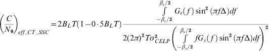
Substituting expression (5) into expression (7) yields:
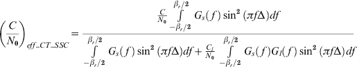
When there is intrasystem and intersystem interference coexistence, the (C/N 0)eff_CT_SSC can be expressed as:
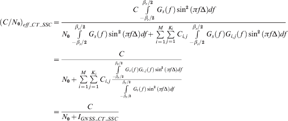
where
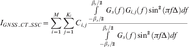
I GNSS_CT_SSC is the aggregate equivalent noise power density of the combination of intrasystem and intersystem interference.
From (9) it is clear that the impact of the interference on (C/N 0)eff_CT_SSC is also directly related to CT_SSC.
When considering a DLL using non-coherent early-late tracking, the variance of the code tracking error (Betz, Reference Betz2000a) is
As we can see the variance of the code tracking error of non-coherent DLL is the product of σCELP2 and a squaring loss, θsquare_loss, that is greater than unity, but approaches unity for the usual range of C/N 0. So in the case of non-coherent DLL (Soualle, Reference Soualle, Kaindl, Hechenblaikner and Middendorf2007b), the same CT_SSC and (C/N 0)eff_CT_SSC can be obtained.
2.2. Equivalent noise power density
When more than two systems are operating together, the aggregate equivalent noise power density I GNSS (I GNSS_SSC or I GNSS_CT_SSC) is the sum of two components:
where I Intra is the equivalent noise power density of interfering signals from satellites belonging to the same system as the desired signal, and I Inter is the aggregate equivalent noise power density of interfering signals from satellites belonging to the other systems.
In fact, recalling the SSC and CT_SSC definitions, hereafter denoted κi,js or ηi,js as γi,js, the equivalent noise power density (I Intra or I Inter) can be simplified as follows:
The user received power C i,j of the j-th signal belonging to the i-th satellite can be written in terms of satellite transmit power, satellite and user receiver antenna gains, space loss and polarization loss (Owen, Reference Owen, Goldstein and Hegarty2002):
where P i,j is the transmit power of the j-th signal belonging to the i-th satellite, L dist is the free-space loss due to the distance between i-th satellite and user, L atm is the loss of the signal due to atmospheric loss, L pol is the polarization mismatch loss, G i is the satellite antenna gain between the i-th satellite to the user receiver, G user is the user receiver antenna gain between the user receiver to the i-th satellite.
The atmospheric loss L atm is estimated to be 0·5 dB for all systems (Titus, Reference Titus, Betz, Hegarty and Owen2003). The satellite antenna gain G i is a function of the off-boresight angle α (Wallner, Reference Wallner, Hein, Pany, Avila-Rodriguez and Posfay2005), and is illustrated in Figure 1. It must be noted that different signals from Galileo and Compass have different satellite antenna gain profiles. For example, a typical profile of GPS Block IIA satellite antenna gain is depicted in Figure 2.

Figure 1. Illustration of off-boresight angle.

Figure 2. Typical satellite antenna gain.
The free-space loss L dist can be expressed as:
where c is the speed of light, d is the distance between satellite and user, and f 0 is the carrier centre frequency.
For the aggregate equivalent noise power density calculation, the constellation configuration, satellite and user receiver antenna gain patterns, and the space loss are included in the link-budget equation. User receiver location must be taken into account when measuring the interference effects. When a receiver at a given location m on the Earth at any time over a 24-hour period, the aggregate equivalent noise power density to a desired signal s can be written as follows:
Equation (16) is the sum of all equivalent noise power density from all signals of all satellites in view at any time. When the desired satellite is used, it must be subtracted from the power spectral density of the desired signal from the desired satellite.
2.3. Degradation of effective C/N0
A general way to calculate (C/N 0)eff ((C/N 0)eff_SSC or (C/N 0)eff_CT_SSC) introduced by interfering signals from satellites belonging to the same system or other systems is based on equation (1) or (8). In addition to the calculation of (C/N 0)eff, calculating degradation of effective C/N 0 is more interesting when more than two systems are operating together. The degradation of effective C/N 0 in the case of the intersystem interference is:

Therefore, the expression of intersystem interference in dB as:
For example, if Galileo and Compass are operating together, regarding Galileo E1 OS signal on the i-th satellite as the desired satellite and the desired signal, I Intra and I Inter can be expressed as:
Where I E1OS,others is the equivalent noise power density of Galileo E1 OS signal belonging to the other satellites of the Galileo constellation.
3. SIMULATION PARAMETERS
This section provides the space constellations and signals parameters of Galileo and Compass for computer simulations.
3.1. Space constellations
The space constellation parameters of Galileo and Compass are summarized in the Table 1. Galileo will be composed of 30 satellites in three orbital planes, with 27 operational spacecraft and three in-orbit spares (1/plane) (ICD-Galileo, 2008). Here we take the 27 satellites for Galileo constellation. Compass will consist of 27 MEO satellites, five GEO and three IGSO satellites (China, 2006, Liu, Reference Liu, Zhai, Zhang and Zhan2009). Due to the fact that Galileo and Compass are under construction, ideal constellation parameters are taken from Table 1 and the Galileo and Compass space constellations are shown in Figure 3.

Figure 3. Galileo and Compass space constellations.
Table 1. Space constellation parameters.

3.2. Signal parameters
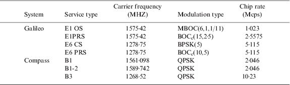
The frequency bands of Galileo and Compass are shown in Figure 4. It can be seen that a lot of attention must be paid to the signal spectrum overlaps at E1/B1 and E6/B3 bands between these systems. Thus, we will concentrate the interference only on the E1/B1 and E6/B3 bands in this paper. All satellite signals which include (i) the Galileo E1 PRS, E1OS, E6 CS and E6 PRS signals, (ii) the Compass B1, B1-2 and B3 signals will be taken into account in the simulations. Table 2 summarizes the characteristics of Galileo and Compass signals to be transmitted in E1/B1 and E6/B3 bands (Avila-Rodriguez, Reference Avila-Rodriguez, Hein and Wallner2007, Liu, Reference Liu, Zhai, Zhang and Zhan2009). The detailed information about the signal parameters can be found in the Galileo interface control document and International Telecommunication Union (ITU) related document (China, 2006, ICD-Galileo, 2008). The power spectral densities of the Galileo and Compass signals in E1/B1 and E6/B3 bands are shown in Figure 5 and Figure 6, respectively.

Figure 4. Galileo and Compass frequency bands.

Figure 5. PSD of the Galileo and Compass signals in E1/B1 band.

Figure 6. PSD of the Galileo and Compass signals in E6/B3 band.
Table 2. Galileo and Compass signal parameters in E1/B1 and E6/B3 bands.
4. SIMULATION RESULTS
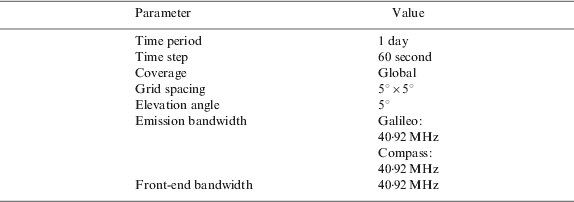
Table 3 summarizes the simulation parameters which are simulated for the aggregate equivalent noise power densities. Here, we assume a transmitter filter bandwidth of 40.92 MHz for the Galileo and Compass signals so that at least one of the secondary lobes falls inside it.
Table 3. Simulation parameters.
We can see from equation (1) or (8) that (C/N 0)eff is directly related to SSC or CT_SSC of the desired and interfering signals. Figure 7 shows both SSC and SSC for the different interfering signals and for a Galileo E1 OS as desired signal. It obviously shows that CT_SSC is significantly different from the SSC. It also shows that CT_SSC depends on the early-late spacing and its maximal values appear at different early-late spacing.

Figure 7. SSC and CT_SSC for Galileo E1 OS as desired signal.
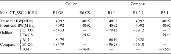
The CT_SSC for different civil signals in E1/B1 and E6/B3 bands are calculated using equation (4). The power spectral densities are normalized to the transmitter filter bandwidth and integrated in the bandwidth of the user receiver. As we saw in equation (4), when calculating the CT_SSC, it is necessary to consider all possible values of early-late spacing. In order to determine the maximum equivalent noise power density (I Intra or I Inter), the maximum CT_SSC will be calculated within the typical early-late spacing ranges (0·1– 1chip space). The results are shown in Table 4. If we compare the maximum CT_SSC and the SSC, the maximum CT_SSC can vary up to 9·2 dB for the pair of Compass B1-I as desired and Galileo E1OS as interfering signal.
Table 4. Code tracking spectral sensitivity coefficients in E1/B1 and E6/B3 bands.

All intersystem interference simulations refer to the worst scenarios. The worst scenarios assume minimum emission power for the desired signal, maximum emission power for all interfered signals and maximum (C/N 0)eff degradation of interference over all time steps. The maximum and minimum received power of Galileo and Compass in the bands of interest – E1/B1 and E6/B3 – can be found in (China, 2006, Liu, Reference Liu, Zhai, Zhang and Zhan2009). In this paper we only show the results of the worst scenarios where Galileo and Compass are sharing the same band. The worst scenarios include:
• Scenario 1: Galileo E1 OS←Compass B1 and B 1-2 (Galileo E1 OS is interfered by Compass)
• Scenario 2: Compass B1-I←Galileo E1 OS and E1 PRS (Compass B1-I is interfered by Galileo)
• Scenario 3: Compass B1-2-I←Galileo E1 OS and E1 PRS (Compass B1-2-I is interfered by Galileo)
• Scenario 4: Galileo E6 CS←Compass B3 (Galileo E6 CS is interfered by Compass)
It must be noted that we only display all civil signals' interference results. Therefore, because Compass B3 signal belongs to an authorized signal, the result of Compass B3 signal interfered by Galileo is not displayed in this paper.
4.1. Galileo and Compass intersystem interference on E1/B1 band
Figure 8 shows the maximum (C/N 0)eff_CT_SSC degradation of Galileo signal due to Compass intersystem interference on E1/B1 band (Scenario 1). As can be seen, Galileo E1 OS signal maximum (C/N 0)eff_CT_SSC degradation is raised from 0·0213 dB to 0·0369 dB. The maximum (C/N 0)eff_CT_SSC degradations of Compass B1-I and B1-2-I signals interfered by Galileo signals in E1/B1 band (Scenario 2 and Scenario 3) are shown in Figure 9 and Figure 10. We can obtain the maximal value of 2·8462 dB and 2·8515 dB of Compass B1-I and B1-2-I signals, respectively.

Figure 8. Max (C/N 0)eff_CT_SSC degradation of Galileo E1 OS Signal due to Compass intersystem interference on E1/B1 band.

Figure 9. Max (C/N 0)eff_CT_SSC degradation of Compass B1-I Signal due to Galileo intersystem interference on E1/B1 band.

Figure 10. Max (C/N 0)eff_CT_SSC degradation of Compass B1-2-I Signal due to Galileo intersystem interference on E1/B1 band.
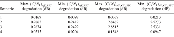
Figures 8–10 show that the maximal values of Galileo interfered by Compass are lower than Galileo interfering with Compass on E1/B1 band. If we compare the result of (C/N 0)eff_CT_SSC with (C/N 0)eff_SSC, we can clearly see that the maximal value of (C/N 0)eff_CT_SSC degradation is approximately 0·02 dB higher than the maximal value of (C/N 0)eff_SSC degradation when Galileo E1 OS is interfered by Compass. The (C/N 0)eff_SSC results are shown in (Liu, Reference Liu, Zhai, Zhang and Zhan2009). When Compass B1-I and B1-2-I signals are interfered by Galileo signals, all the maximal values of (C/N 0)eff_SSC degradation are around 0·2865 dB and 0·2874 dB for Compass B1-I and B1-2-I signal, respectively. Obviously, as can be seen from Table 5, the maximal values of (C/N 0)eff_CT_SSC degradation are much higher than the maximal values of (C/N 0)eff_SSC degradations. This is because the maximum CT_SSC is 11·123 dB higher than the SSC of the pair of Compass B1-I as desired and Galileo E1 PRS as interfering signal, resulting in the higher I Inter in the intersystem interference computation. It is also shown that the maximum interference Galileo had suffered induced by Compass on E1/B1 band is below 0·25 dB using existing rules of coordination at ITU.
Table 5. Effective carrier power to noise density degradations based on SSC and CT_SSC.

4.2. Galileo and Compass intersystem interference on E6/B3 band
Figure 11 shows the maximum (C/N 0)eff_CT_SSC degradation of Galileo signal due to Compass intersystem interference on E6/B3 band (Scenario 4). Compared with Figure 8, it can be seen that the Galileo E6 CS signal (C/N 0)eff_CT_SSC degradation is approximately 0·1179 dB higher than that of Galileo E1 OS signal. Again, If we compare the result of (C/N 0)eff_CT_SSC with (C/N 0)eff_SSC listed in Table 5, we can clearly see that the maximal value of (C/N 0)eff_CT_SSC degradation is approximately 0·1213 dB higher than the maximal value of (C/N 0)eff_SSC degradation when Galileo E6 CS is interfered by Compass.

Figure 11. Max (C/N 0)eff_CT_SSC degradation of Galileo E6 CS signal due to Compass Intersystem Interference on E6/B3 band.
With the results from the above simulation results, it is clear that the Compass system leads to intersystem interference on Galileo and that the maximal values are lower than those of Galileo interfering on Compass. The results also show that the effects of interfering signals on code tracking performance may be underestimated in the former radio frequency compatibility methodologies.
CONCLUSIONS
The exponentially increasing number of navigation systems, hand-in-hand with the new signals, including civil, commercial, and military signals, result in the need to assess radio frequency compatibility carefully. The design and implementation of any new signal has to be conducted carefully in order to avoid interferences. In other words, all GNSS signals and services must be compatible.
In this paper, a more complete methodology based on the SSC and CT_SSC for the radio frequency compatibility assessment has been described. A detailed derivation of the methodology including equations and computation principle are provided. This methodology takes into account the space constellation, signal modulation, emission power level, space loss, satellite antenna gain and user receiver characteristic. Real simulations are carried out to assess the interference effects where Galileo and Compass signals are sharing the same band (E1/B1 and E6/B3 bands) at every time and place on the Earth. Simulation results show that the effects of intersystem interference are significantly different by using these two methodologies. The effects of interfering signals on code tracking performance must be considered in the radio frequency compatibility assessment. It is also shown that the Compass system leads to intersystem interference on Galileo and the maximum values are lower than Galileo interference on Compass.
Finally it has to be pointed out that the intersystem interference results shown in this paper refer mainly to the worst scenario simulations. Although the value is higher than normal it is feasible for GNSS system interference assessment. It must also be noted that PRN codes have impact on the PSD, e.g. short PRN code. And the effects of Doppler differences on the SSC and CT_SSC also need to be considered in future work.
ACKNOWLEDGEMENT
This work has been sponsored by the National High Technology under the following contracts: 2009AA12Z322.