2. DEVELOPMENT OF A MULTI-CONSTELLATION MULTI-FREQUENCY GNSS SIMULATOR

In order to evaluate the future performance of Galileo in PPP, on its own and together with GPS, in this research a multi-constellation GNSS simulator was developed in the Simulink environment.

The inputs that are required to run a simulation are:

• • Reference trajectory for user motion. This includes a time series of the user's latitude, longitude and height at each epoch. In case the output data rate is higher than the input data rate, an interpolation between points is performed to obtain the user's position at the required epoch.

• • Information about satellites' motion and clocks' offset and drift. For GPS satellites, this information is obtained from the Yuma almanac, while for Galileo, the nominal orbital parameters of the Galileo constellation are used.

• • Klobuchar parameters to model the Ionospheric delay.

The simulator outputs GNSS observations in Receiver Independent Exchange (RINEX) 2·11 observation format.

Code pseudoranges $P_{r\comma k}^{s}$ and carrier phases $L_{r\comma k}^{s}$ on frequency k, broadcast by satellite s and received by the receiver r, are simulated considering the main delays as shown in Teunissen and Montenbruck (Reference Teunissen and Montenbruck2017).

(1)$$P_{r\comma k}^{s} = g_{r}^{s}+c\lpar \hbox{d}t_{r}-dt^{s}+\delta t^{rel}\rpar +c\lpar d_{r\comma k}-d_{k}^{s} \rpar +I_{r\comma k}^{s}+T_{r}^{s}+\varepsilon_{P\comma r\comma k}^{s} $$

(2)$$L_{r\comma k}^{s} = g_{r}^{s}+c\lpar \hbox{d}t_{r}-dt^{s}+\delta t^{rel} \rpar -I_{r\comma k}^{s}+T_{r}^{s}+\lambda_{k}N_{r\comma k}^{s}+\varepsilon_{L\comma r\comma k}^{s} $$

In Equations (1) and (2), the generic measurement equations for pseudorange and carrier phase, the geometric range is $g_{r}^{s}$, the receiver and satellite clock offsets are dt _r and dt ^s, the relativistic effect is δ t ^rel, the speed of light is c, the frequency dependant instrumental delay for the receiver is d _{r, k} and for the satellites is $d_{k}^{s}$ and the atmospheric delay due to the ionosphere is $I_{r\comma k}^{s}$ and troposphere is $T_{r}^{s}$. The carrier phase initial ambiguity is $N_{r\comma k}^{s}$ the wavelength of the carrier signal on frequency k is λ_k and other errors like receiver noise and multipath are $\varepsilon_{P\comma r\comma k}^{s}$ and $\varepsilon_{L\comma r\comma k}^{s}$.

The pseudorange receiver noise ε_PR has been modelled as a white Gaussian noise (normally distributed with zero mean) with a standard deviation σ_PR depending on the Signal to Noise Ratio (SNR). The model is based on the results presented in Richardson et al. (Reference Richardson, Hill and Moore2016).

(3)$$\varepsilon_{PR}=N\lpar 0\comma \; \sigma_{PR}^{2}\rpar $$

The exponential law of σ_PR as function of the SNR is shown in Figure 1: Galileo pseudoranges seem to be less noisy than the GPS ones. The carrier phases are assumed to have a precision of 1 cm.

Figure 1. Receiver noise for different GPS and Galileo signals as function of the SNR (Richardson et al., Reference Richardson, Hill and Moore2016).

Multipath is modelled as a first order Gauss-Markov process (O'Keefe et al., Reference O'Keefe, Petovello, Lachapelle and Cannon2006) with a correlation time τ which depends on the type of simulation. It is larger for static scenarios and shorter for kinematic scenarios.

(4)$$\varepsilon_{mp_{k}}=w_{k}+\varepsilon_{mp_{k-1}}e^{-\displaystyle{{\Delta t}\over{\tau}}} $$

In Equation (4), $\varepsilon_{mp_{k}}$ is the GaussMarkov process being generated at epoch k, Δ t is the observation rate, and w _k is the driving noise term simulated using a normally distributed random number generator with a standard deviation that is assumed to be a function of the elevation angle of the satellite.

As illustrated in Simsky et al. (Reference Simsky, Mertens, Sleewaegen, Hollreiser and Crisci2008), the Galileo E1 and E6 and GPS L1 are the signals most affected by multipath interference, while the Galileo Alternative Binary Offset Carrier (AltBOC) modulated signal, E5, is the least affected. Based on these results, three multipath groups were defined: a high multipath group, which includes all the signals that are more sensitive to multipath (Galileo E1, E6 and GPS L1, L2); a medium multipath group (Galileo E5a, E5b and GPS L5) and a low multipath group (Galileo E5). The standard deviation of the assumed multipath for each group is shown in Figure 2 together with the assumed carrier phase multipath.

Figure 2. Magnitude of the multipath delays as a function of the elevation angle. The high multipath group (blue) includes the Galileo E1 and E6 and GPS L1 and L2 pseudoranges. The medium multipath group (orange) includes the Galileo E5a, E5b and GPS L5 pseudoranges. The low multipath group (yellow) includes Galileo E5 pseudoranges. The multipath on the carrier phase measurements is also shown in purple.

The simulator also outputs Real-Time quality precise orbits and clocks in Standard Products 3 (SP3) and RINEX clock 2·0 formats. The model to simulate the products' error is based on the comparison between the GPS IGS Real-Time and ESA Final products. Data relative to four weeks (GPS week 1917 to 1920) have been analysed in order to define a suitable model.

The Crustal Dynamics Data Information System (CDDIS) archives products generated from a real-time data stream in support of the IGS Real-Time Service. The precise orbits files are published in SP3 format at 30 second intervals, while the precise clocks files are in RINEX clock format at 30 second intervals. They are derived from the IGC01 solution, which uses the real-time data streams that are referred to the satellite centre-of-mass (CoM). The ESA Final orbits, which are published at 15 minutes intervals, have been interpolated to reduce the data interval to 30 seconds.

Table 1 shows the Root Mean Square (RMS) of the products' differences. The RMS of the clocks' differences are almost twice as large as those presented in Hadas and Bosy (Reference Hadas and Bosy2015), while the radial, cross-track and along-track orbital components have nearly the same RMS.

Table 1. Root Mean Square (RMS) of the products' difference during the period analysed.

Figure 3 shows the daily time series of the orbital component differences for GPS PRN 1 on 2 October 2016. These plots clearly show a periodic pattern on all components. Two peculiar patterns are also visible in the cross-track and along-track components. The authors could not explain the reason for this behaviour.

Figure 3. Difference between the IGS Real-Time and ESA Final orbits for GPS PRN 1 on 2 October 2016. The upper plot shows the products' difference in the radial component of the satellite's position, the middle plot shows the difference in the cross-track component, while the lower one shows the difference on the along-track component.

Figure 4 shows the difference between the IGS Real-Time clocks and the ESA Final clocks for GPS PRN 1 on 2 October 2016. A drift is visible in the daily time series. This behaviour is related to the way the products are computed.

Figure 4. Difference between IGS Real-Time and ESA Final clocks for GPS PRN 1 on 2 October 2016.

When estimating the clocks, a reference needs to be defined. The Final products are computed by processing seven days of data; the clock of a station at a particular epoch is considered as the reference for the computation of all the other clocks for that week. On the other hand, the Real-Time products are computed, independently, epoch by epoch. Therefore, while the reference clock for the Real-Time products is assumed to be zero at each epoch, in the Final products it drifts with time. This drift is visible when differentiating the two types of precise clocks. To overcome this problem, a single difference process between satellites' clocks is performed, in such a way that we always use the same satellite's clock as the reference.

Given the periodical nature of the products' errors, a fitting method based on the Fourier series was used to characterise them.

(5)$$\Delta_{RT}=a_{0}+\sum\limits_n a_{n}\sin \lpar n\omega t+\Phi_{n} \rpar $$

In Equation (5), a ₀ is the bias, a _n is the amplitude, nω is the frequency and Φ_n is the phase of the sinusoid of order n.

To study what frequency has to be used in the fitting, the spectrum of the products' error was analysed. Figures 5 and 6 present the spectrum of the orbits for GPS PRN 5 and PRN 14.

Figure 5. Spectrum of the error in the radial, along-track, and cross-track orbit components. PRN 5. On the x-axis the frequencies are in units of 1/ day.

Figure 6. Spectrum of the error in the radial, along-track, and cross-track orbit components. PRN 14. On the x- axis the frequencies are in units of 1/ day.

A peak at a frequency of twice per day is visible in all the orbit components, while a peak at once per day is mainly in the along-track direction. Smaller peaks are also at three to eight times per day, but they were neglected in our modelling.

Similar conclusions can be drawn by looking at the spectrum of the clocks' difference. Hence, the error in the Real-Time products Δ_RT is modelled as the sum of two sinusoids with period T _E equal to the Earth rotation Period (23 hours 56 minutes) and period T _O equal to the orbital period of the constellation (11 hours 58 minutes for GPS, 14 hours 22 minutes for Galileo).

(6)$$\Delta_{RT}=b+a_{E}\sin \left(\displaystyle{{2\pi}\over{T_{E}}}t+\Phi_{E}\right)+a_{O}\sin \left(\displaystyle{{2\pi}\over{T_{O}}}t+\Phi_{O}\right)$$

Table 2 shows the average biases and amplitudes a _E and a _O for each component in the period analysed.

Table 2. RMS of the fitting parameters. a _E is the amplitude of the sinusoid with period equal to the Earth rotation period, while a _O is the amplitude of the sinusoid with period equal to the orbital period of the constellation.

3. VALIDATION

The system was validated against real data recorded between GPS week 1917 and 1920. GPS observations from ten stations (Figure 7) within the IGS global network were considered. Each daily RINEX file was split into two six hours data arcs (0 – 6am, 12 – 6pm) and, therefore, 560 data points were analysed.

Figure 7. IGS stations considered for validation.

The POINT software was used to process the GNSS observations in PPP mode. This software, which was developed in the iNsight project (www.insight-gnss.org), supports multiple constellations (GPS, GLONASS, and Galileo) and multiple positioning techniques, such as Real Time Kinematic (RTK) and PPP (Jokinen et al., Reference Jokinen, Feng, Ochieng, Hide, Moore and Hill2012).

The metric used to analyse the positioning performance are the errors in the north, east and down components of the position at the end of the six hours, and the time they take to converge to below one decimetre. Tables 3 and 4 show that the performance of the Simulink model is comparable to the real data.

Table 3. Median of the positioning errors for simulated and real data. Values in units of centimetres.

Table 4. Median of convergence times for simulated and real data. Values in units of minutes.

4. MULTI-CONSTELLATION PPP RESULTS

The PPP solutions based on the Ionosphere Free (IF) combination between GPS L1 and L5 signals only, Galileo E1 and E5a or E1 and E5 only, and combined GPS and Galileo signals are analysed. The simulated observations from the same ten stations as in the validation stage were processed with the POINT software in static mode with float ambiguity Open sky conditions were assumed. The simulator was run 55 times for each station.

For static processing, the metrics used to define the positioning performance are the errors in the north, east and down components of the position at the end of the processing and the time these errors take to converge below 10 cm level.

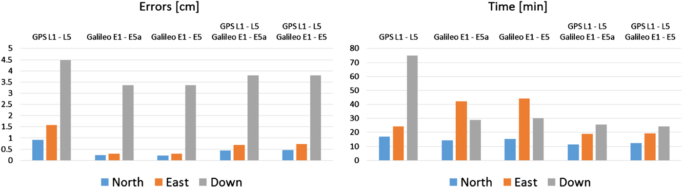
Figures 8 and 9 show a comparison between the RMS of the errors and convergence times for each position's component and for the different signals combinations for station PERT and HLFX.

Figure 8. Errors and convergence times for different signals combinations: in the first block is GPS L1 – L5 IF, the second refers to Galileo E1 – E5a IF, in the third is Galileo E1 – E5 IF, in the fourth is GPS L1 – L5 IF plus Galileo E1 – E5a IF, and the last block is GPS L1 – L5 IF plus Galileo E1 – E5 IF. Station PERT.

Figure 9. Errors and convergence times for different signals combinations: in the first block is GPS L1 – L5 IF, the second refers to Galileo E1 – E5a IF, in the third is Galileo E1 – E5 IF, in the fourth is GPS L1 – L5 IF plus Galileo E1 – E5a IF, and the last block is GPS L1 – L5 IF plus Galileo E1 – E5 IF. Station HLFX.

Each combination is able to provide sub-decimetre level accuracy after a few tens of minutes. The convergence time in the vertical direction is usually the longest, it ranges from 24 minutes for the multi-constellation solution to 75 minutes for GPS L1 – L5 IF, both in HLFX.

In eight stations out of the ten considered, positioning with Galileo E1 – E5a IF performs better than GPS L1 – L5 IF, both in terms of accuracy and convergence time. Up to 33% and 29% of improvement, respectively, in the down accuracy level and convergence time can be observed when processing the Galileo E1 – E5a IF compared to GPS L1 – L5 IF. PERT is the only station where GPS outperforms Galileo in both vertical accuracy and convergence time, while at FFMJ Galileo has worse vertical accuracy but faster convergence time than GPS. The reason why Galileo, in general, performs so much better than GPS has to be attributed to the lower noise that was assumed in the code pseudoranges (Richardson et al., Reference Richardson, Hill and Moore2016).

Given the open sky conditions, there were not many improvements in terms of Dilution of Precision (DOP) when the two constellations were used together with respect to the single constellation case (see Figure 10), therefore the accuracy achieved is mostly sensitive to the quality of the pseudoranges. For this reason, it is mainly the convergence time that benefits from using GPS and Galileo together. On average over all the considered stations, the convergence time was 47% faster than the GPS-only solution and 26% faster than the Galileo-only solution.

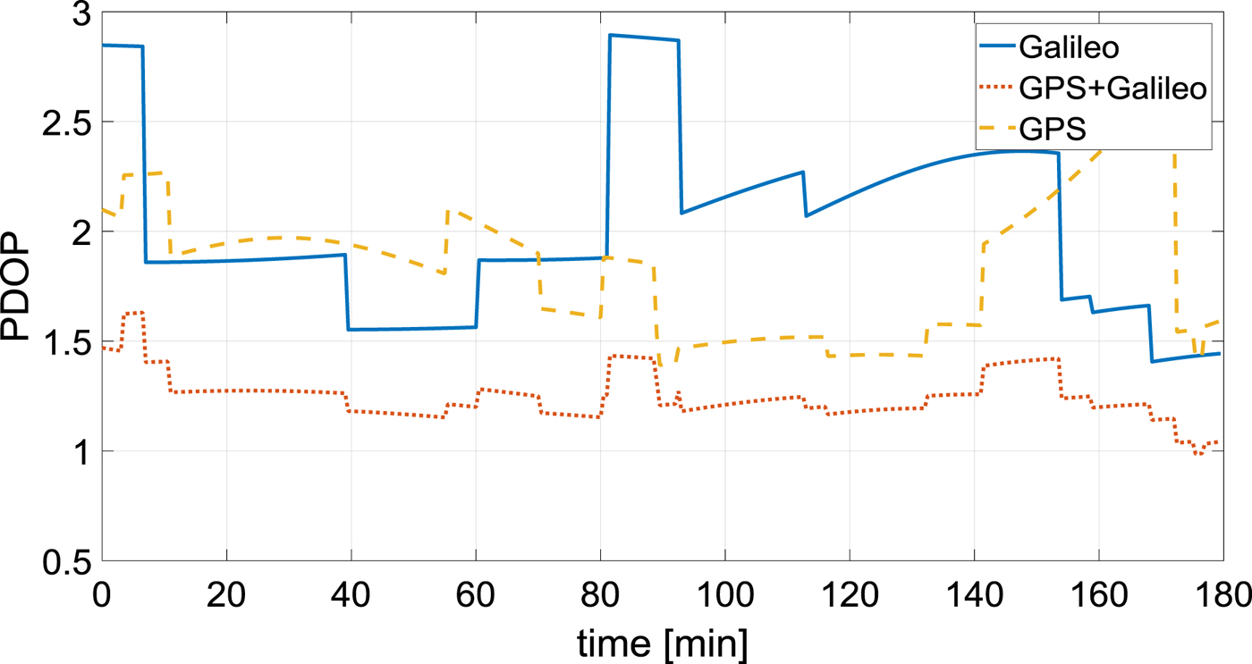
Figure 10. Galileo-only, GPS-only and GPS plus Galileo Position Dilution of Precision (PDOP). Station HLFX.

By employing the Galileo E1 – E5 IF no benefits to the positioning solution were registered in comparison with the E1 – E5a solution. From simulated analysis, the two combinations have nearly the same performance. The reason can be found in the IF combination, which is well known to degrade the quality of the measurements.

5. CONCEPT OF SMOOTHED IONOSPHERE CORRECTION FOR FAST RE-CONVERGENCE

In order to shorten the convergence time, ambiguity fixing methods have been developed in recent years (Collins et al., Reference Collins, Bisnath, Lahaye and Héroux2010; Laurichesse et al., Reference Laurichesse, Mercier, Berthias, Broca and Cerri2009; Ge et al., Reference Ge, Gendt, Rothacher, Shi and Liu2008). These methods are all based on ionosphere free combination.

However, the results presented in the previous section demonstrate that the convergence time in PPP would be shorter if we could use less noisy pseudoranges. Therefore, the use of the IF combination, which can amplify the noise in the measurements up to three times, limits the potential performance of PPP. Obviously, this is accepted as it is the best option available to mitigate the ionospheric delay in the observables. As an alternative, PPP algorithms in which the ionospheric delays were provided by Global Ionospheric Map (GIM) (Teunissen et al., Reference Teunissen, Odijk and Zhang2010; Wubbena et al., Reference Wubbena, Schmitz and Bagge2005) or estimated in the state vector (Geng et al., Reference Geng, Meng, Dodson, Ge and Teferle2010; Li et al., Reference Li, Ge, Zhang and Wickert2013; Zhang et al., Reference Zhang, Gao, Ge, Niu, Huang, Tu and Li2013) were proposed. The performance of these approaches not only depends on the quality of the GIM or the spatial and temporal constraints used for the ionosphere estimation, but also on a careful handling of the Differential Code Biases (DCBs), as pointed out in Zhang et al. (Reference Zhang, Gao, Ge, Niu, Huang, Tu and Li2013).

Here a new method to mitigate the ionosphere and aimed to reduce the re-convergence time, after initial convergence has been achieved, is proposed. Re-convergence is important in situations such as mobile platforms operating in urban environments.

The IF combination P ₃ between two pseudoranges P ₁ and P ₂ on frequencies f ₁ and f ₂ can be computed according to Equation (7):

(7)$$P_{3}=\displaystyle{{f_{1}^{2}}\over{f_{1}^{2}-f_{2}^{2}}}P_{1}-\displaystyle{{f_{2}^{2}}\over{f_{1}^{2}-f_{2}^{2}}}P_{2} $$

This formulation is equivalent to correcting the pseudorange P ₁ with the ionospheric delay $I_{1}^{P}$ computed from the geometry free combination

(8)$$P_{3}=P_{1}-I_{1}^{P} $$

(9)$$I_{1}^{P} = \displaystyle{{P_{1}-P_{2}}\over{1-\displaystyle{{f_{1}^{2}}\over{f_{2}^{2}}}}}$$

In this new method, the ionospheric correction is smoothed through a Hatch filter (Hatch Reference Hatch1982) before being applied to the pseudorange. The opposite sign of the ionospheric delay in the code pseudorange and carrier phase needs to be considered to avoid the divergence problem (McGraw et al., Reference McGraw, Schnaufer, Hwang and Armatys2013). In Equation (10), Ĩ _{1, k} is the smoothed ionosphere at epoch k, $I_{1\comma k}^{P}$ is the ionosphere parameter computed from the pseudoranges at epoch k, according to Equation (9), $I_{1\comma k}^{L}$ is the ionosphere parameter computed from the carrier phase measurements, as in Equation (11). Finally n is the size of the smoothing window.

(10)$$\tilde{I}_{1\comma k} = \displaystyle{{1}\over{n}}I_{1\comma k}^{P}+\left(1-\displaystyle{{1}\over{n}} \right)\cdot \lpar \tilde{I}_{1\comma k-1}+\lpar I_{1\comma k}^{L}-I_{1\comma k-1}^{L} \rpar $$

(11)$$I_{1\comma k}^{L} = -\displaystyle{{L_{1}-L_{2}}\over{1-\displaystyle{{f_{1}^{2}}\over{f_{2}^{2}}}}} $$

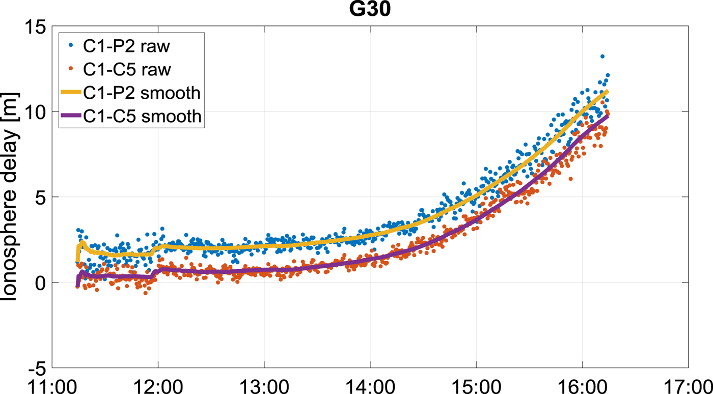
In this way, we can choose a smoothing window as large as the whole observation period without being affected by the divergence, as demonstrated in Figure 11.

Figure 11. Ionosphere delay computed from C1 – P2 combination (raw blue dots, smoothed yellow line) and C1 – C5 combination (raw orange dots, smoothed purple line). GPS PRN 30 observed from BOGT on 6 September 2016. On that day a minor solar storm made the ionosphere active. The offset between the two plots is due to the DCBs.

Once the Hatch filter has converged, ideally we have IF pseudoranges with up to three times less noise than the traditional IF combination.

In case the receiver loses track of all the satellites and the PPP filter needs to be restarted, we can take advantage of this new low noise IF pseudorange to obtain a quicker re-convergence, rather than having tens of minutes with metre or decimetre level accuracy. Indeed, provided that the signal gap is not very large, the Hatch filter applied to the ionosphere delay does not need to be reinitialised from the raw values if a cycle slip occurs. The old information about how the ionosphere changes with time can be used to propagate even in case of a cycle slip, since the change of rate of the ionosphere does not vary that much from epoch to epoch.

6. PRELIMINARY RESULTS

To test the benefit of this new method on the reconvergence time, three hours of simulated Galileo data were processed with the POINT software in kinematic mode. After 90 minutes, the PPP filter was forced to restart to simulate reconvergence. The performance of the traditional E1 – E5 IF were compared with those of E1 and E5 corrected with smoothed ionosphere delay coming from the Hatch filter. Figures 12, 13 and 14 show the precision (3σ) of the north, east and down components after filter restart. In all three components, the new approach shows faster re-convergence with respect to the traditional PPP based on the IF combination.

Figure 12. Comparison between the accuracy level provided by the traditional E1 – E5 IF, the E1 plus Hatch filter configuration and the E5 plus Hatch configuration after the PPP filter was forced to restart. North component. The standard deviation at epoch e is computed between e and e plus 30 minutes.

Figure 13. Comparison between the accuracy level provided by the traditional E1 – E5 IF, the E1 plus Hatch filter configuration and the E5 plus Hatch configuration after the PPP filter was forced to restart. East component. The standard deviation at epoch e is computed between e and e plus 30 minutes.

Figure 14. Comparison between the accuracy level provided by the traditional E1 – E5 IF, the E1 plus Hatch filter configuration and the E5 plus Hatch configuration after the PPP filter was forced to restart. Down component. The standard deviation at epoch e is computed between e and e plus 30 minutes.

In particular, the horizontal components for the E5 plus Hatch case converge below 10 cm accuracy immediately. The vertical component takes only 240 seconds to reach an accuracy of 25 cm for 99% of the time, against 900 seconds for the E1 – E5 IF combination. Big improvements are also visible if we consider the noisier E1 signal. The horizontal components re-converge to below 10 cm in less than 200 seconds and the vertical component takes 700 seconds to go below 25 cm.