


1. INTRODUCTION
Measurements made by global navigation satellite systems (GNSS) are vulnerable to faults, including satellite and constellation failures, which can potentially lead to catastrophic consequences in safety-critical applications (Pervan, Reference Pervan1996). To mitigate their impact, receiver autonomous integrity monitoring (RAIM) fault detection has been designed and implemented in aviation as a backup navigation tool (Lee, Reference Lee1986; Parkinson and Axelrad, Reference Parkinson and Axelrad1988; RTCA Special Committee 159, 1991). RAIM uses global positioning system (GPS) only, where it exploits redundant measurements to detect single satellite fault at the user receiver (Joerger et al., Reference Joerger, Chan and Pervan2014).
Future multi-constellation GNSS is anticipated to provide dramatically increased measurement redundancy (Gibbons, Reference Gibbons2012). In addition, the application of dual-frequency signals will remove the largest measurement error caused by ionospheric delay. Moreover, the satellite clock and ephemeris errors have been significantly reduced since 2010 (Walter et al., Reference Walter, Gunning, Phelts and Blanch2018), which in turn improves navigation accuracy. These developments in GNSS have opened the possibility of achieving worldwide vertical guidance for aircraft using the RAIM concept. Therefore, advanced RAIM (ARAIM) fault detection and exclusion methods have recently attracted considerable research interest, especially in the European Union and in the United States (Federal Aviation Administration (FAA), 2010; Blanch et al., Reference Blanch, Walter, Enge, Lee, Pervan, Rippl, Spletter and Kropp2015; EU-US Cooperation, 2015; Zhai et al., Reference Zhai, Joerger and Pervan2018).
The achievable performance of RAIM/ARAIM, as measured in terms of either integrity risk or protection level at the airborne receiver, is highly dependent on the assumed GNSS nominal signal-in-space (SIS) error models and on the a-priori fault probabilities (Joerger et al., Reference Joerger, Chan and Pervan2014; Blanch et al., Reference Blanch, Walter, Enge, Lee, Pervan, Rippl, Spletter and Kropp2015). In current RAIM implementations, this information is defined by the GPS constellation service provider (CSP) commitments and is hardcoded in the receiver (Lee et al., Reference Lee, Van Dyke, DeCleene, Studenny and Beckmann1996). As an evolution of RAIM, ARAIM will (a) use constellations that are not as mature as GPS, and (b) seek to provide assured navigation for vertical guidance, i.e., evaluating not only the horizontal but also the vertical protection level (FAA, 2010).
Figure 1 presents the ARAIM architecture. Unlike RAIM, ARAIM relies on a broadcast integrity support message (ISM) to specify SIS error and fault statistics (Blanch et al., Reference Blanch, Walter, Enge, Lee, Pervan, Rippl, Spletter and Kropp2015). The ISM parameters will be generated and validated at the ground, and updated to users as needed (EU-US Cooperation, 2015). Various methods of ISM dissemination are presently being considered, including on-aircraft databases and data broadcast through one or more of the GNSS core constellations. The methods and results described in this paper are applicable regardless of the means of dissemination.
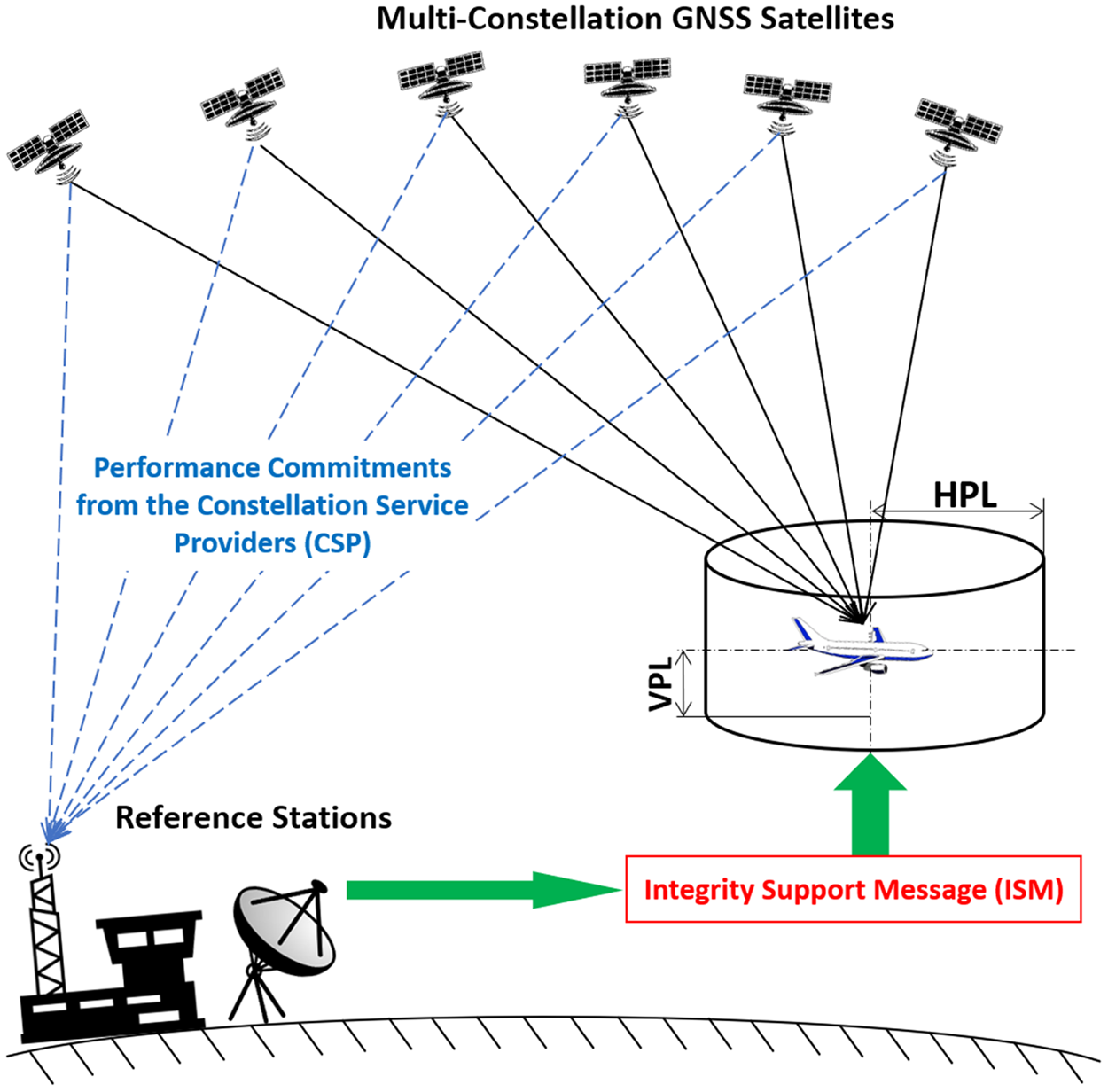
Figure 1. ARAIM architecture.
To validate the ISM, prior research has taken truth satellite positions and clock biases from the International GNSS Service (IGS) network (Walter and Blanch, Reference Walter and Blanch2015; Perea et al., Reference Perea, Meurer, Rippl, Belabbas and Joerger2017; Walter et al., Reference Walter, Gunning, Phelts and Blanch2018). However, given that ARAIM is intended to operate over several decades, the dependence of monitoring on external systems or organisations, such as IGS, that have little or no stake in civil aviation, must be carefully considered, and ideally, avoided. Most importantly, ARAIM is intended for safety-critical applications; any potential safety threat must be properly accounted for and quantified. The IGS, the National Geospatial Intelligence Agency (NGA), and others currently provide highly accurate satellite orbit/clock products. But none of these agencies make specific commitments on the reliability of their products or on the processes used to obtain those products. Further, data gaps exist in those products, especially during satellite fault events, which are crucial to ARAIM. In response, this paper develops a new approach to generate ‘truth’ satellite orbits/clocks for ARAIM offline monitoring (OFM). This approach provides the air navigation service provider with more insight and more control over the OFM process compared with relying on IGS or NGA products.
In the new monitor design, measurements are collected from a worldwide network of sparsely distributed reference stations (RS). A parametric orbit model is used to fit data over time. Two estimators are considered: a Kalman filter (KF), and a batch least-squares method. In both cases, satellite orbits, satellite clock biases, and RS clock biases are simultaneously estimated by incorporating either the GPS legacy or the GPS civil navigation (CNAV) orbit models, which were both designed to be accurate over 4 h intervals (US Air Force, 2013).
Satellite orbit and clock errors are determined by differencing the position and timing solutions derived from the GNSS-broadcast navigation message and the ‘truth’ product generated by the OFM. Then, in the ISM generator, the errors will be used to evaluate the ISM parameters (Walter et al., Reference Walter, Gunning, Phelts and Blanch2018). On the one hand, the ISM parameters must include enough margin to bound the actual constellation performance over the specified period of ISM validity (e.g., one month). On the other hand, the ISM parameters should not be set too conservatively or ARAIM availability will be degraded. Therefore, it is essential that the ground monitor be capable of producing tight bounds on satellite position and clock estimation errors. In this work, a two-step evaluation of the estimated orbit and clock accuracy is carried out: first, the impact of measurement errors at RS receivers is quantified by covariance analysis, and second, the fidelity of the orbit model is validated by computing the model residuals relative to known satellite positions.
This paper is organised as follows. Section 2 introduces the OFM concept and the required performance. Sections 3 and 4 describe the OFM architecture and the estimator design, respectively. Section 5 presents the results of the two analyses. Section 6 concludes this paper.
2. OFM CONCEPT AND REQUIRED PERFORMANCE
To generate the ISM, ‘online’ and ‘offline’ ARAIM architectures are considered (Blanch et al., Reference Blanch, Walter, Enge, Pervan, Joerger, Khanafseh, Burns, Alexander, Boyero, Lee, Kropp, Milner, Macabiau, Suard, Berz and Rippl2014; EU-US Cooperation, 2015; Joerger et al., Reference Joerger, Zhai and Pervan2015; Khanafseh et al., Reference Khanafseh, Joerger, Chan and Pervan2015). The offline architecture, which is of primary interest in this work, does not require a real-time communication link between users and ground segment. Offline ARAIM therefore reduces the connectivity risk (EU-US Cooperation, 2015). In offline ARAIM, the ISM update period may vary from a month to a year, and the processes of ISM generation and validation are closely related. An ISM generator determines integrity bounds on SIS performance, which must remain valid until the next time update. The OFM either confirms that the bounds are valid, or indicates that a change in parameter values is needed at the next update.
To bound the instantaneous user ranging error (IURE) under nominal, fault-free conditions, a scaling factor α on the broadcast standard deviation of the user ranging accuracy (URA)  $\sigma_{{\rm URA}} $ is defined in ARAIM ISM (EU-US Cooperation, 2015). The bound can then be specified as a Gaussian distribution with a mean of the nominal ranging bias b nom and a standard deviation of
  $\alpha \sigma_{{\rm URA}}$ (Walter et al., Reference Walter, Gunning, Phelts and Blanch2018). In this paper, we focus on producing satellite orbit and clock estimates to validate α and b nom. Since the monitor's orbit/clock estimation errors directly contribute to the validated ISM, it is necessary first to define the required accuracy of the OFM's orbit/clock estimator.
Equation (1) shows the relationship between the actual overbounding standard deviation of the IURE  $\sigma_{\hbox{OB, IURE}}$, the standard deviation of the monitor's estimated orbit/clock error
  $\sigma_{{\rm OFM}}$, and the validated standard deviation of the satellite orbit/clock error
  $\alpha \sigma_{{\rm URA}}$:
 $$\alpha \sigma_{{\rm URA}} =\sqrt {\sigma_{{\rm OB,IURE}}^2 +\sigma_{{\rm OFM}}^2}$$
 Figure 2 plots  $\alpha \sigma_{{\rm URA}}$ versus
  $\sigma_{{\rm OFM}}$ over different
  $\sigma_{\hbox {OB, IURE}}$ values. We focus on the red curve because it is expected that future performance of the GPS constellation will provide
  $\sigma_{\hbox {OB, IURE}}$ lower than 1 m. The figure shows slow growth of
  $\alpha \sigma_{{\rm URA}}$ as
  $\sigma_{{\rm OFM}}$ increases. Even when
  $\sigma_{{\rm OFM}}$ reaches 0·5 m, i.e., half of the
  $\sigma_{\hbox{OB, IURE}}$ value, the achievable validated
  $\alpha \sigma_{{\rm URA}}$ remains below 1·1 m. For an actual
  $\sigma_{\hbox{OB, IURE}}$ of 1 m, a
  $\sigma_{{\rm OFM}}$ of 0·3 meter would achieve a
  $\alpha \sigma_{{\rm URA}}$ around 1·03 m.

Figure 2. Validated user range accuracy  $( {\alpha \sigma_{{\rm URA}}} ) $ versus monitor accuracy
  $( {\sigma_{{\rm OFM}} } ) $ for varying values of σOB, IURE.
In addition to α, the nominal ranging bias b nom in ISM captures the effects of signal deformation, inter-frequency bias error, code-carrier incoherence, and/or satellite antenna biases. The value of b nom is highly dependent on specific receivers, and its evaluation had been characterised in Walter et al. (Reference Walter, Gunning and Blanch2017) and Walter et al. (Reference Walter, Gunning, Phelts and Blanch2018). Using the proposed OFM, the estimated satellite orbit/clock error may have a non-zero mean, denoted by b OFM. This term will be accounted as a component of the validated b nom. b nom is a particularly sensitive parameter for ARAIM availability performance because it contributes to the user protection level in the worst-conspiring way (Blanch et al., Reference Blanch, Walter, Enge, Lee, Pervan, Rippl, Spletter and Kropp2015). Therefore, we want to keep contributions of b OFM to the validated b nom as low as possible. As a result, we will mainly use  $\sigma_{{\rm OFM}}$ to address the impact of measurement error and orbit model error on the estimated satellite orbit/clock. Evaluating the b OFM value requires experimental data, which will be considered in our future work.
The above analysis shows that the accuracy of the OFM does not need to be nearly as high as the precise satellite orbit/clock products by IGS or NGA – which claim accuracy in the order of 5 cm. Instead, for use in safety-critical applications, the ability to quantify and bound the OFM's estimator performance is key. Therefore, in this work, we design a simple and transparent orbit/clock estimator, which is sufficient to validate the ISM.
3. OFM ARCHITECTURE
This section describes the OFM architecture. A network of worldwide sparsely distributed RS is employed to collect code and carrier measurements over time. We select OFM RS co-located with existing space-based augmentation system (SBAS) ground infrastructure, which is intended to support civil aviation applications. Figure 3 (left) shows all existing SBAS RS from the US Wide Area Augmentation System (WAAS), the European Geostationary Navigation Overlay Service (EGNOS), the Japanese Multi-functional Satellite Augmentation System (MSAS), the Indian GPS-Aided GEO Augmented Navigation (GAGAN) and the Russian System for Differential Corrections and Monitoring. Figure 3 (right) shows the 20 RS locations selected in this work. To obtain a roughly uniform global distribution, five non-SBAS RS sites from the NGA and the US Air Force are added. This network ensures that each satellite can be tracked continuously by at least two RS but does not allow reverse positioning (four RS simultaneously observing a space vehicle (SV) are required to estimate the satellite position directly). Instead, the OFM uses parametric orbit models to determine SV trajectories.

Figure 3. Existing SBAS stations (left) and example network of 20 RS selected in this work (right).
We consider two candidate medium Earth orbit (MEO) SV orbit models, the GPS legacy and CNAV models. The former uses 15 orbit parameters versus 17 for the latter (US Air Force, 2013). Throughout this paper, we assume that no satellite manoeuvre occurs because orbit models would not be valid during spacecraft thrusting. Manoeuvres occur rarely and can be handled separately in the offline monitor (e.g., by initiating a new estimator once the manoeuvre is completed). Such practical considerations are beyond the scope of this work.
Let  $\textbf{p}_{i}^{{\rm orb}}$ be the 15 × 1 (or 17 × 1, depending on which orbit model is used) vector of orbit model parameters for SV i. The true SV position
  $\textbf{x}_{i, k} $ of SV i at time epoch k in an Earth-centred Earth-fixed (ECEF) reference frame can be expressed as:
 $$\textbf{x}_{i,k} = \textbf{g}_{{\rm orb},k} (\textbf{p}_i^{{\rm orb}} )+\boldsymbol{\nu}_{i,k}^{{\rm orb}}$$
 where  $\textbf{g}_{{\rm orb}, k} $ is the non-linear function that relates
  $\textbf{p}_{i}^{{\rm orb}} $ to
  $\textbf{x}_{i, k}$ and
  $\boldsymbol{\nu}_{i, k}^{{\rm orb}} $ is the deviation of the model output from the true position
  $\textbf{x}_{i, k} $.
  $\boldsymbol{\nu}_{i, k}^{{\rm orb}} $ represents the model's inability to capture the true orbit perfectly, which is evaluated in later sections. The GPS orbit model is valid over a time interval of 4–6 h noted as T FIT (US Air Force, 2013). Sensitivity to T FIT has been evaluated in our prior work (Joerger et al., Reference Joerger, Zhai and Pervan2015). A fitting interval of 4 h commonly used for GPS ephemerides is used in this work.
Both RS and SV are equipped with atomic clocks, whose nominal biases could be modelled using a quadratic polynomial (US Air Force, 2013). However, in order to monitor SV clocks, which are the main source of SV faults, no assumption can be made on the SV clock dynamics. In parallel, an RS can be equipped with redundant atomic clocks, so any receiver clock faults can be detected and removed. To investigate the potential benefit of using a quadratic RS receiver clock model, two cases are analysed: (a) applying a quadratic polynomial to model RS clock errors, and (b) making no assumption on RS clocks (i.e., estimating RS clock states at each time epoch). Under case (a), let b j, k to be the clock bias of RS j at time k. b j, k can be modelled as:
 $$b_{j,k} =g_{{\rm clk},k} (\textbf{p}_j^{{\rm clk}} )+\nu_{j,k}^{{\rm clk}}$$
 Similar to Equation (2),  $\textbf{p}_{j}^{{\rm clk}}$ in Equation (3) is a 3 × 1 vector of clock parameters including the bias, slope and acceleration coefficients labelled
  $a_{f0}^{j} $,
  $a_{f1}^{j} $,
  $a_{f2}^{j}$ in US Air Force (2013).
  $\nu_{j, k}^{{\rm clk}} $ is the clock model's error.
  ${\rm g}_{{\rm clk}, k} ( {\textbf{p}_{j}^{{\rm clk}} } ) $ is a linear function of clock parameters that can be expressed as:
 $$g_{{\rm clk},k} (\textbf{p}_j^{{\rm clk}} )=a_{f0}^j +a_{f1}^j (t_k-t_{{\rm ref}} )+a_{f2}^j (t_k -t_{{\rm ref}} )^2$$
where t k and t ref respectively are the true time and reference time.
Dual-frequency, ionosphere-free code and carrier measurements for SV i, from RS j, at time epoch k, are expressed as:
 $$\begin{align} { }^{i,j}\rho_k &=\left\| {\textbf{x}_j -\textbf{x}_{i,k} } \right\|-\tau_{i,k} +b_{j,k} +{ }^{i,j}T_k +{ }^{i,j}\varepsilon_{\rho,k}^{{\rm RNM}}\label{eq5} \end{align}$$
 $$\begin{align}{ }^{i,j}\varphi_k &=\left\| {\textbf{x}_j -\textbf{x}_{i,k} }\right\|-\tau_{i,k} +b_{j,k} +{ }^{i,j}\eta +{ }^{i,j}T_k +{}^{i,j}\varepsilon_{\varphi, k}^{{\rm RNM}}\label{eq6} \end{align}$$
where  $\textbf{x}_{j}$ denotes the known location of RS j in ECEF.
  $\textbf{x}_{i, k} $ is the unknown location of SV i at time k. τi, k and b j, k are the unknown clock offsets of SV i and RS j, respectively. i, jη is the carrier phase cycle ambiguity for SV i at RS j.
  $\Vert \Vert $ is the Euclidean norm operator, which designates the distance between RS j and SV i.
The error terms in Equations (5) and (6) account for the receiver noise and multipath (RNM), which are noted  ${ }^{i, j}\varepsilon_{\rho, k}^{{\rm RNM}} $ for code and
  ${ }^{i, j}\varepsilon_{\phi, k}^{{\rm RNM}} $ for carrier. We assume that raw, single frequency code and carrier RNM errors are bounded by Gaussian distributions with zero mean and standard deviations of 0·5 m and 0·01 m, respectively. These standard deviations are multiplied by 2·588 to account for the ionosphere-free combination at L1 and L5 frequencies.
For the tropospheric delay i, jT k, we consider the ‘UNB3m’ neutral atmosphere model (developed by the University of New Brunswick, Fredericton, Canada) (Leandro et al., Reference Leandro, Santos and Langley2006). The residual zenith tropospheric delay (ZTD)  $( {\varepsilon_{{\rm tropo}, j, k}^{{\rm ZTD}}}) $ of this model has a standard deviation of 0·05 m. This value is scaled for lower elevation satellites using the tropospheric mapping function
  $( {c_{T}}) $ given in Blanch et al. (Reference Blanch, Walter, Enge, Lee, Pervan, Rippl, Spletter and Kropp2015) and RTCA Special Committee 159 (2006). To account for the temporal and spatial correlation of ZTD, we employ a first-order Gauss-Markov process (FOGMP) with a 30 min correlation time (RTCA Special Committee 159, 2006). Let
  ${ }^{i, j}\varepsilon _{{\rm tropo}, k} $ be the residual tropospheric delay. i, jT k is expressed as:
 $$\begin{align} { }^{i,j}T_k &={ }^{i,j}T_k^{{\rm model}} +{ }^{i,j}\varepsilon_{{\rm tropo},k} \\ &={ }^{i,j}T_k^{{\rm model}} +c_T { }^{i,j}\varepsilon_{{\rm tropo},k}^{{\rm ZTD}} \\ \end{align}$$
 To estimate the SV orbit and clock parameters, the measurement Equations (5) and (6) and the orbit/clock model Equations (3) and (4) can be linearised and incorporated into a single filter. The following derivation is presented for code measurements only, but exactly the same steps are followed to linearise carrier phase observations (not shown here). The code measurement Equation (5) is linearised about an initial guess  $\textbf{x}_{i, k}^{\ast} $ of the position of SV i at time k. The linearised code measurement can be written as:
 $$\begin{align} { }^{i,j}\delta \rho_k &={ }^{i,j}\rho_k -\left\| {\textbf{x}_j -\textbf{x}_{i,k}^\ast } \right\|-{ }^{i,j}T_k^{{\rm model}} \\ &={ }^{i,j}\textbf{e}_k^T \boldsymbol{\delta} \textbf{x}_{i,k} -\tau_{i,k}+b_{j,k} +{ }^{i,j}\varepsilon_{\rho, k} \\ \end{align}$$
 where  $\boldsymbol{\delta}$ denotes the deviation from nominal values, e.g.,
  $\delta \textbf{x}_{i, k} =\textbf{x}_{i, k} -\textbf{x}_{i, k}^{\rm \ast } $.
  ${ }^{i, j}\textbf{e}_{k}$ is the 3 × 1 line of sight (LOS) unit vector from RS j to SV i at time k in ECEF.
  ${ }^{i, j}\varepsilon_{\rho, k} $ is the code measurement error, and is the sum of
  ${ }^{i, j}\varepsilon_{{\rm tropo}, k} $ and
  ${ }^{i, j}\varepsilon_{\rho, k}^{{\rm RNM}} ( {{ }^{i, j}\varepsilon_{\rho, k} ={ }^{i, j}\varepsilon_{{\rm tropo}, k} +{ }^{i, j}\varepsilon_{\rho, k}^{{\rm RNM}} } ) $.
In the next step, the orbit model is linearised about an initial guess of the orbit parameters  ${ }^{\ast}\textbf{p}_{i}^{{\rm orb}}$ where
  $\textbf{x}_{i, k}^{\ast} =\textbf{g}_{{\rm orb}, k} ( {{}^{\ast}\textbf{p}_{i}^{{\rm orb}} } ) $. Substituting the linearised orbit model equation and the clock error model Equation (4) into the code measurement, Equation (8) becomes:
 $${ }^{i,j}\delta \rho_k ={ }^{i,j}\textbf{e}_k^T \textbf{A}_{i,k}^{{\rm orb}} \boldsymbol{\delta} \textbf{p}_i^{{\rm orb}} -\tau_{i,k} +\textbf{A}_{j,k}^{{\rm clk}} \textbf{p}_j^{{\rm clk}} +{}^{i,j}\varepsilon_{\rho, k}$$
 where  $\textbf{A}_{i, k}^{{\rm orb}} $ is the Jacobian matrix for the SV orbit model in Equation (2), which is 3 × 15 for the GPS legacy orbit model and 3 × 17 for the CNAV model. It is composed of numerically-derived partial derivatives of the position coordinates of SV i at time
  $k \left(\textbf{x}_{i, k} =\left[\begin{smallmatrix} {x_{i, k} } & {y_{i, k} } & {z_{i, k} }\end{smallmatrix}\right]^{T}\right)$ with respect to the orbit parameters
  $\textbf{p}_{i}^{{\rm orb}} =\left[\begin{smallmatrix} {p_{1} } & \cdots & {p_{15} } \end{smallmatrix}\right]^{T}$:
 $$\textbf{A}_{i,k}^{{\rm orb}} =\left[\begin{matrix} {{\partial x_{i,k} } / {\partial p_1 }} & {{\partial y_{i,k} }/ {\partial p_1 }} & {{\partial z_{i,k} } /{\partial p_1 }} \\ \vdots & \vdots & \vdots \\ {{\partial x_{i,k} } / {\partial p_{15} }} & {{\partial y_{i,k} } / {\partial p_{15}}} & {{\partial z_{i,k} } /{\partial p_{15} }} \\ \end{matrix}\right]^T$$
 and  $\textbf{A}_{j, k}^{{\rm clk}} $ is a 1 × 3 vector that can be used to express Equation (4) in matrix form:
 $$\textbf{A}_{j,k}^{{\rm clk}} =\left[\begin{matrix} 1 & {(t_k -t_{{\rm ref}} )} & {(t_k -t_{{\rm ref}} )^2}\end{matrix}\right]$$
 It is worth noting that we opted to perform two linearisation steps in Equations (8) and (9) rather than a single step because matrices  $\textbf{A}_{j, k}^{{\rm orb}} $,
  $\textbf{A}_{j, k}^{{\rm clk}} $ and
  ${ }^{i, j}\textbf{e}_{k} $ will separately be used again later in Section 5, and because this two-step approach is numerically more stable.
4. ESTIMATOR DESIGN
Based on the linearised measurement Equation (9), we can derive the estimator. The parameters to be estimated or ‘states’ include SV orbit parameters  $\delta \textbf{p}_{i}^{{\rm orb}} $, SV clock bias τi, k, RS clock model parameters
  $\textbf{p}_{j}^{{\rm clk}} $, cycle ambiguities i, jη, and residual tropospheric delay
  ${}^{i, j}\varepsilon_{{\rm tropo}, j, k}^{{\rm ZTD}} $. All of these states can be estimated simultaneously using either a KF or batch implementation. The KF approach is presented in this section, and the alternative batch approach is provided in Appendix A. The states are estimated over a fit interval T FIT of 4 h. To avoid modelling correlation between samples due to RS multipath, the sample period must be longer than the correlation time of multipath. There has been prior work analysing the multipath profiles under various conditions, suggesting the time constant is well below 200 s (Joerger, Reference Joerger2009; Pervan et al., Reference Pervan, Khanafseh and Patel2017; Khanafseh et al., Reference Khanafseh, Kujur, Joerger, Walter, Pullen, Blanch, Doherty, Norman, Groot and Pervan2018). Therefore, a sample period of 4 min, which is long enough to decorrelate the multipath errors, is employed in this work. In addition, to enable state observability, clock error states including both SV and RS clocks are measured with respect to the clock of RS 1. It is worth clarifying that an external clock standard is required to generate an absolute clock reference. For the purpose of analysis in this paper, it is assumed that we have access to such standard, but this assumption needs to be validated when prototyping this design using experimental data (e.g., using the averaged clock estimate as the standard).
 $$\begin{align} \left[\begin{matrix} {{ }^{1,1}\delta \rho_k }\\ {{ }^{1,2}\delta \rho_k }\\ \vdots\\ {{ }^{1,J}\delta \rho_k }\\ \vdots\\ {{ }^{i,j}\delta \rho_k }\\ \vdots\\ {{ }^{I,J}\delta \rho_k }\\ {{ }^{1,1}\delta \phi_k }\\ \vdots\\ {{ }^{I,J}\delta \phi_k }\\\end{matrix}\right]&=\left[\begin{array}{*{20}c} {{ }^{1,1}\textbf{B}_k }& \cdots& \textbf{0}_{1\times 15} & {-1}& \cdots& 0& \textbf{0}_{1\times 3} & \cdots& \textbf{0}_{1\times 3} & 0& \cdots& 0& {c_T }& 0&\cdots& 0\\ {{ }^{1,2}\textbf{B}_k }& \cdots& \textbf{0}_{1\times 15} & {-1}& \cdots& 0& {\textbf{A}_{2,k}^{{\rm clk}} }& \cdots& \textbf{0}_{1\times 3} & 0& \cdots& 0& 0&{c_T }& \cdots& 0\\ \vdots&& \vdots& \vdots&& \vdots && \ddots&& \vdots&& \vdots & \vdots&& \ddots&\\ {{ }^{1,J}\textbf{B}_k }& \cdots& \textbf{0}_{1\times 15} & {-1}& \cdots& 0& \textbf{0}_{1\times 3} & \cdots& {\textbf{A}_{J,k}^{{\rm clk}} }& 0& \cdots& 0& 0 & \cdots& 0& {c_T }\\ & \ddots& \vdots&& \ddots&& & \ddots&& \vdots&& \vdots& & \ddots&&\\ \textbf{0}_{1\times 15} & {{ }^{i,j}\textbf{B}_k \,\cdots } & \textbf{0}_{1\times 15} & 0& {-1\,\cdots } & 0& \textbf{0}_{1\times 3}& {\textbf{A}_{j,k}^{clk} \,\cdots }& \textbf{0}_{1\times 3} & 0 & \cdots& 0& 0& {c_T }& \cdots& 0\\ \vdots& \ddots&& \vdots& \ddots& && \ddots&& \vdots&& \vdots & \vdots&& \ddots&\\ \textbf{0}_{1\times 15} & \cdots& {{ }^{I,J}\textbf{B}_k }& 0& \cdots& {-1}& \textbf{0}_{1\times 3} & \cdots& {\textbf{A}_{J,k}^{{\rm clk}}}& 0& \cdots& 0& 0& \cdots&0& {c_T }\\ {{ }^{1,1}\textbf{B}_k }& \cdots& \textbf{0}_{1\times 15}& {-1}& \cdots& 0& \textbf{0}_{1\times 3} & \cdots& \textbf{0}_{1\times 3} & 1& \cdots& 0& {c_T }& 0&\cdots& 0\\ & \ddots&&& \ddots&& \vdots & \ddots&&& \ddots&&&\ddots&&\\ \textbf{0}_{1\times 15} & \cdots& {{ }^{I,J}\textbf{B}_k }& 0& \cdots& {-1}& \textbf{0}_{1\times 3} & \cdots& {\textbf{A}_{J,k}^{{\rm clk}}}& 0& \cdots& 1& 0& \cdots&0& {c_T }\\ \end{array}\right] \nonumber \\ &\quad\times \left[\begin{matrix} {\delta \textbf{p}_1^{{\rm orb}} }\\ \vdots\\ {\delta \textbf{p}_I^{{\rm orb}} }\\ {\tau_{1,k} }\\ \vdots\\ {\tau_{I,k} }\\ {\textbf{p}_2^{{\rm clk}} }\\ \vdots\\ {\textbf{p}_J^{{\rm clk}} }\\ { }^{1,1}\eta \\ \vdots \\ { }^{I,J}\eta \\ {\varepsilon_{t{\rm ropo},1,k}^{{\rm ZTD}} }\\ \vdots\\ {\varepsilon_{{\rm tropo},J,k}^{{\rm ZTD}} }\\ \end{matrix}\right] +\left[\begin{matrix} {{ }^{1,1}\varepsilon_{\rho, k}^{{\rm RNM}} }\\ {{ }^{1,2}\varepsilon_{\rho, k}^{{\rm RNM}} }\\ \vdots\\ {{ }^{1,J}\varepsilon_{\rho, k}^{{\rm RNM}} }\\ \vdots\\ {{ }^{i,j}\varepsilon_{\rho, k}^{{\rm RNM}} }\\ \vdots\\ {{ }^{I,J}\varepsilon_{\rho, k}^{{\rm RNM}} }\\ {{ }^{1,1}\varepsilon_{\varphi, k}^{{\rm RNM}} }\\ \vdots\\ {{ }^{I,J}\varepsilon_{\varphi, k}^{{\rm RNM}} }\\ \end{matrix}\right] \end{align}$$
 In this KF implementation, code and carrier measurements at time epoch k, for all SVs at all RSs, are stacked together in a measurement vector. Let I and J respectively be the total number of SVs and RSs (SV index i ranges from 1 to I, and RS index j ranges from 1 to J). The measurement equation at time k is given in Equation (12). Five groups of states and their corresponding observation matrix coefficients are distinguished by thin dashed lines. In Equation (12), 0a×b is an a × b matrix of zeros, and the product of the LOS unit vector and the Jacobian matrix in Equation (9) is defined as  ${ }^{i, j}\textbf{B}_{k} $, i.e.,
  ${ }^{i, j}\textbf{B}_{k} ={ }^{i, j}\textbf{e}_{k}^{T}\ \textbf{A}_{i, k}^{{\rm orb}} $. For clarity of explanation, Equation (12) does not capture the fact that satellites come in and out of sight of different RS at different times. In practice, rows corresponding to out-of-view SVs at each RS must be removed.
Let us simplify Equation (12) by defining  $\textbf{z}_{k} $,
  $\textbf{H}_{k} $,
  $\textbf{s}_{k} $, and
  $\boldsymbol{\varepsilon}_{k}$ be the measurement vector, observation matrix, state vector, and error vector, respectively. The KF measurement equation can be expressed as:
 $$\textbf{z}_k =\textbf{H}_k \textbf{s}_k +\boldsymbol{\varepsilon}_k$$
 The measurement error vector  $\boldsymbol{\varepsilon}_{k}$ includes RNM contributions. The time correlation of the tropospheric error
  $\varepsilon_{{\rm tropo}, j}^{{\rm ZTD}} $ is incorporated by state augmentation in Equation (12) (Brown and Hwang, Reference Brown and Hwang2012). Because
  $\varepsilon_{{\rm tropo}, j}^{{\rm ZTD}} $ is modelled as a FOGMP, the associated dynamic model of the KF approach is written as:
 $$\begin{align} &\left[\begin{matrix} {\delta \textbf{p}^{{\rm orb}}}\\ \boldsymbol{\tau}_{k+1} \\ {\textbf{p}^{{\rm clk}}}\\ \boldsymbol{\eta}\\ \boldsymbol{\varepsilon}_{{\rm tropo},k+1}^{{\rm ZTD}} \\ \end{matrix}\right]\nonumber\\ &\quad =\left[\begin{matrix} {\textbf{I}_{\left( {15\times I} \right)\times \left( {15\times I}\right)} } & \textbf{0}_{\left( {15\times I} \right)\times I} & \textbf{0}_{\left( {15\times I} \right)\times \left[ {\left( {J-1}\right)\times 3} \right]} & \textbf{0}_{\left( {15\times I}\right)\times \left( {I\times J} \right)} & \textbf{0}_{\left({15\times I} \right)\times J} \\ \textbf{0}_{I\times \left( {15\times I} \right)} & {\textbf{I}_{I\times I} } & \textbf{0}_{I\times \left[ {\left( {J-1}\right)\times 3} \right]} & \textbf{0}_{I\times \left( {I\times J}\right)} & \textbf{0}_{I\times J} \\ \textbf{0}_{\left[ {\left( {J-1} \right)\times 3} \right]\times \left({15\times I} \right)} & \textbf{0}_{\left[ {\left( {J-1} \right)\times 3} \right]\times I} & {\textbf{I}_{\left[ {\left( {J-1} \right)\times 3} \right]\times \left[ {\left( {J-1} \right)\times 3} \right]} } & \textbf{0}_{\left[ {\left( {J-1} \right)\times 3} \right]\times \left({I\times J} \right)} & \textbf{0}_{\left[ {\left( {J-1} \right)\times 3} \right]\times J} \\ \textbf{0}_{\left( {I\times J} \right)\times \left( {15\times I} \right)} & \textbf{0}_{\left( {I\times J} \right)\times I} & \textbf{0}_{\left( {I\times J} \right)\times \left[ {\left( {J-1} \right)\times 3} \right]} & {\textbf{I}_{\left( {I\times J} \right)\times \left( {I\times J} \right)} } & \textbf{0}_{\left( {I\times J} \right)\times J} \\ \textbf{0}_{J\times \left( {15\times I} \right)} & \textbf{0}_{J\times I} & \textbf{0}_{J\times \left[ {\left( {J-1} \right)\times 3} \right]} & \textbf{0}_{J\times \left( {I\times J} \right)} & {e^{{-T}/ \mu }\textbf{I}_{J\times J} } \\ \end{matrix}\right]\nonumber \\ &\qquad\times \left[\begin{matrix} {\delta \textbf{p}^{{\rm orb}}}\\ {\boldsymbol{\tau}}_k \\ {\textbf{p}^{{\rm clk}}}\\ {\boldsymbol{\eta}}\\ {\boldsymbol{\varepsilon}}_{{\rm tropo},k}^{{\rm ZTD}} \\ \end{matrix}\right]+\left[\begin{matrix} \textbf{0}_{\left( {15\times I} \right)\times I} & \textbf{0}_{\left( {15\times I} \right)\times J} \\ {\textbf{I}_{I\times I} } & \textbf{0}_{I\times J} \\ \textbf{0}_{\left[ {\left( {J-1} \right)\times 3} \right]\times I} &\textbf{0}_{\left[ {\left( {J-1} \right)\times 3} \right]\times J} \\ \textbf{0}_{\left( {I\times J} \right)\times I} & \textbf{0}_{\left( {I\times J} \right)\times J} \\ \textbf{0}_{J\times I} & {\textbf{I}_{J\times J} } \\ \end{matrix}\right]\left[\begin{matrix} \boldsymbol{\omega}_\tau \\ \boldsymbol{\omega}_{{\rm tropo},k}^{{\rm ZTD}} \\ \end{matrix}\right] \end{align}$$
which takes the following standard form:
 $$\boldsymbol{s}_{k+1} =\boldsymbol{\Phi} \textbf{s}_k +\boldsymbol{\Gamma \omega}_k$$
 In Equation (14),  $\textbf{I}_{a\times a} $ is an a × a identity matrix. State vector components are grouped together, as expressed in the following equations:
 $$\delta \textbf{p}^{{\rm orb}}=\left[\begin{matrix} {\delta \textbf{p}_1^{{\rm orb}} }\\ \vdots\\ {\delta \textbf{p}_I^{{\rm orb}} }\\ \end{matrix}\right],\quad \boldsymbol{\tau}_k =\left[ \begin{matrix} {\tau_{1,k} }\\ \vdots\\ {\tau_{I,k} }\\ \end{matrix}\right],\quad \textbf{p}^{{\rm clk}}=\left[ \begin{matrix} {\textbf{p}_2^{{\rm clk}} }\\ \vdots\\ {\textbf{p}_J^{{\rm clk}} }\\ \end{matrix}\right],\quad \boldsymbol{\eta}=\left[ \begin{matrix} {{ }^{1,1}\eta }\\ \vdots\\ {{ }^{I,J}\eta }\\ \end{matrix} \right]$$
 The FOGMP is expressed in the last row in Equation (14), where T is the sample period and μ is the time constant (Gelb, Reference Gelb2001).  $\boldsymbol{\varepsilon}_{{\rm tropo, }k}^{{\rm ZTD}} $ is obtained by stacking
  $\varepsilon_{{\rm tropo}, j, k}^{{\rm ZTD}} $ of all RS, and the variance of
  $\omega_{{\rm tropo}, k}^{{\rm ZTD}} $ is
  $( {1-e^{-2( {T/\mu} ) }}) \sigma_{{\rm ZTD}}^{2} $ (Joerger, Reference Joerger2009). Even though
  $\delta \textbf{p}_{i}^{{\rm orb}} $,
  $\textbf{p}_{i}^{{\rm clk}} $, and η are constant over time, we do not know how τk changes over time. Because no model is assumed for the SV clock, large process noise is modelled, that is, ωτ is modelled as a zero-mean Gaussian function with standard deviation approaching infinity.
Because there are not enough measurements to observe all the states at the beginning steps of the filter, the KF is implemented in information form. A forward information filter is first implemented to estimate the optimal SV orbit parameters. A backward filter is then applied to obtain optimal SV clock estimates at each sample time epoch k over the fit interval T FIT (Crassidis and Junkins, Reference Crassidis and Junkins2004). Compared with the KF design in our prior work (Zhai et al., Reference Zhai, Kiarash, Jamoom, Joerger and Pervan2017; Zhai, Reference Zhai2018) and, where all the clock states at all time epochs are always kept in the KF process, this approach takes a more compact form. Since the number of SV clock states is reduced from I × K (prior approach) to I (new approach), the computational and memory efficiency is significantly improved. As a result, the estimated SV orbit parameters  $\delta \textbf{p}''$ and clock τ ″ can be extracted from the estimated state vector
  $\textbf{s}''$, and the SV position is obtained using Equation (2).
The above derivation was carried out for the legacy GPS orbit model and for RS clock errors modelled as quadratic functions of time. For cases that will be analysed in the next section, where the CNAV orbit model is used and/or where no model is assumed for RS clocks, the expressions of Equations (12) and (14) need to be modified. An example case is investigated in Appendix B to present how the modifications should be made.
5. OFM PERFORMANCE ANALYSIS
This section is structured around the two main sources of OFM SV orbit/clock estimation errors: (a) measurement errors and (b) residual model errors. To address their respective impacts, two separate analyses are carried out. First, assuming that the orbit models are perfect, the contribution of code and carrier measurement errors is evaluated by covariance analysis. Then, assuming that measurements are perfect, we quantify the fidelity of orbit models to actual data.
5.1. Covariance analysis
This analysis investigates the contributions of the measurement errors on  $\sigma_{{\rm OFM}} $. Let
  $\boldsymbol{\Sigma}$ be the covariance matrix of the full-state estimate vector s″. The covariance matrix
  $\textbf{D}_{i, k} $ of the satellite orbit/clock state estimates for SV i at time epoch k is obtained by extracting elements of
  $\boldsymbol{\Sigma}$ for the corresponding states.
  $\textbf{D}_{i, k} $ is a 16 × 16 matrix if the legacy orbit model is employed (15 orbit parameter states plus one clock state at time k). The 4 × 4 covariance matrix
  $\textbf{P}_{LL, i, k}$ of satellite position and clock in the Local-Level (LL) reference frame (along-track, cross-track, radial) is then evaluated using the following equation:
 $$\textbf{P}_{LL,i,k} =\left[\begin{matrix} \textbf{R}_{LL,i,k}& 0\\ 0& 1\\ \end{matrix}\right]\textbf{C}_{i,k} \textbf{D}_{i,k} \textbf{C}_{i,k}^T \left[\begin{matrix} \textbf{R}_{LL,i,k} & 0\\ 0& 1\\ \end{matrix}\right]^T$$
 where  $\textbf{R}_{LL, i, k} $ is the ECEF to LL rotation matrix, and
  $\textbf{C}_{i, k} $ is defined as:
 $$\textbf{C}_{i,k} =\left[\begin{matrix} {\textbf{A}_{i,k}^{{\rm orb}} }& 0\\ 0& 1\\ \end{matrix}\right]$$
 To investigate SIS performance for any user near the Earth's surface, we evaluate the maximum SIS ranging error (SISRE) standard deviation at the worst-case user location. This is achieved by projecting  $\textbf{P}_{LL, i, k} $ along LOS for all locations within the SV footprint (Walter and Blanch, Reference Walter and Blanch2015). In Figure 4, the projection region is shaded in light blue, and the black dashed line is one example projection vector
  $\textbf{G}_{i, m} $, where m is the vector's index. The maximum SISRE variance
  $\sigma_{{\rm SISRE}, i, k}^{2} $ is defined as:
 $$\sigma_{{\rm SISRE},i,k}^2 =\mathop {\max }\limits_{m=1,\ldots {\rm ALL}}\left( \textbf{G}_{i,m} \textbf{P}_{LL,i,k} \textbf{G}_{i,m}^T\right)$$
To explore the potential benefits of employing orbit/clock models to the estimation process, the covariance analyses are performed under four scenarios using:
• in Case 1, a legacy orbit model and a quadratic RS clock model
• in Case 2, a legacy orbit model and no RS clock model
• in Case 3, a CNAV orbit model and a quadratic RS clock model, and
• in Case 4, a CNAV orbit model and no RS clock model.

Figure 4. Overview of the geometry between a satellite and user locations within its footprint.
In the following analyses, we consider code and carrier measurements collected over 4 h fitting intervals T FIT at regular 1 h starting times over one day.
Figure 5 shows profiles of SV clock/orbit estimation error standard deviations over one fitting interval for an example satellite (PRN 5), under Case 1 (left) and Case 4 (right). In each figure, the thin blue lines represent the orbit error deviations for the along-track component (dotted), cross-track (dashed), and radial (solid). The thin black line is the satellite clock error deviation. The thick red line is the worst-case SISRE standard deviation, evaluated using Equation (19).

Figure 5. Profiles of SV clock/orbit deviations for PRN 5, over an example fitting interval, under Case 1 (left) and Case 4 (right).
Both figures in Figure 5 show that the orbit radial and clock components are similar. They are in fact highly correlated. The resulting  $\sigma _{{\rm SISRE}} $ is significantly smaller than each individual term. This is more obviously captured in the SISRE formulas for error evaluation (instead of variance) in US DOD (2008) and Heng (Reference Heng2012) where orbit radial and clock components are subtracted from each other. When comparing the two figures, even though the orbit radial and clock terms are increased for Case 4, there is no noticeable difference between the
  $\sigma_{{\rm SISRE}}$ curves (red lines). This indicates that the estimation covariance is not sensitive to SV orbit model and RS clock model.
For each fitting interval, we use SV orbit/clock estimates in the central 2 h interval (i.e., between hour 1 and hour 3 in Figure 5), and the estimation performance metric used in this analysis is the maximum  $\sigma_{{\rm SISRE}} $ value within these 2 h.
Figure 6 (left) shows the hourly maximum  $\sigma_{{\rm SISRE}} $ values over one day, for all satellites (colour-coded), under Case 4. The distribution of
  $\sigma_{{\rm SISRE}} $ is shown on the right in Figure 6. The large majority of
  $\sigma_{{\rm SISRE}} $ values are well below 0·25 m, and the maximum
  $\sigma_{{\rm SISRE}} $ is 0·3 m.

Figure 6. Hourly maximum σSISRE values over one day (left) and the histogram of σSISRE (right) for Case 4.
Table 1 summarises the results of covariance analysis, which quantitively express the influence of measurement errors on the estimator performance in terms of maximum  $\sigma_{{\rm SISRE}} $ values. In addition, Table 1 also presents the estimator robustness against orbit and clock models; only small variations in
  $\sigma_{{\rm SISRE}} $ are observed between the four cases. Thus, no significant benefit is obtained by using different orbit/clock models when trying to reduce
  $\sigma _{{\rm SISRE}} $, which is one component of
  $\sigma_{{\rm OFM}} $. As expected, the largest
  $\sigma_{{\rm SISRE}} $ is obtained for Case 4 because it requires estimating the largest number of unknown parameters. Based on these results, we recommend not using a quadratic model for RS clock error: the impact of the RS clock error model on
  $\sigma _{{\rm SISRE}} $ is negligible, and not using it allows for seamless operations in the event of a RS clock fault (because RS clock offsets are estimated at each epoch individually). Therefore, Cases 1 and 3 are no longer investigated in the remainder of the paper. In our next analysis, we evaluate the impact of orbit model errors on the monitor's performance for the GPS legacy and GPS CNAV MEO satellite orbit models.
Table 1. Maximum sSISRE values under four cases defined above.

5.2. Orbit model fidelity analysis
In this subsection, the orbit models (15-parameter GPS legacy versus 17-parameter CNAV) are fitted to actual GPS orbit data which is available online. First, precise IGS data,  $\textbf{x}^{{\rm IGS}}$, are considered true SV positions. Then, the orbit parameters
  $\textbf{p}_{i}^{{\rm orb}} $ are estimated using a non-linear least-squares process (Crassidis and Junkins, Reference Crassidis and Junkins2004). The algorithm is initialised using CSP broadcast ephemeris parameters
  $\textbf{p}''$ as initial guesses. For SV i at time epoch k, the residual errors in ECEF are computed as:
 $$\textbf{r}_{i,k} =\textbf{x}_{i,k}^{{\rm IGS}} -\textbf{g}_{{\rm orb},k} (\hat{\textbf{p}}_i^{{\rm orb}} )$$
 where  $\textbf{p}''$ is the estimated orbit parameter vector. Finally,
  $\textbf{r}_{i, k} $ can be expressed in the satellite LL frame as:
 $$\textbf{r}_{LL,i,k} =\textbf{R}_{LL,i,k} \textbf{r}_{i,k} =[\begin{matrix} {r_{A,i,k} }& {r_{C,i,k} }& {r_{R,i,k} }\end{matrix}]^T$$
 In Equation (21), the three components of the right-hand-side vector represent the residual error in three dimensions: along-track, cross-track, and radial. To evaluate the ranging error from  $\textbf{r}_{LL, i, k} $, multiple analytical expressions can be found in the literature (Malys et al., Reference Malys, Larezos, Gottschalk, Mobbs, Winn, Feess, Menn, Swift, Merrigan and Mathon1997; US DOD, 2008; Heng, Reference Heng2012; Perea et al., Reference Perea, Meurer, Rippl, Belabbas and Joerger2017). In this paper, we consider the following equation for orbit-only SISRE:
 $$r_{{\rm SISRE},i,k}^{{\rm orb}} =0\cdot 98r_{R,i,k} +0\cdot24 sgn(r_{R,i,k} )\sqrt {r_{A,i,k}^2 +r_{C,i,k}^2 }$$
Equation (22) is very similar to that used in Heng (Reference Heng2012) except that the SV clock term is removed.
This analysis uses IGS data from 1 January 2016 to 31 January 2016. Similar to the covariance analysis, the data is fitted to the model over T FIT of 4 h, and fitting intervals start at regular 2 h intervals over one day. The sample period is 15 min, and only the central values over 2 h are recorded.
Figure 7 shows the residual SISRE error for an example SV (PRN 5) on 6 January 2016. In each figure, colour coding helps to distinguish fit intervals. Vertical t oe-lines indicate the time of ephemeris, which is at the centre of each 2 h window. The results show that the residual SISRE of the CNAV orbit model is significantly smaller than that of the legacy orbit model.

Figure 7. Best fit residual SISRE orbit over one day: legacy model (left), CNAV model (right).
Figures 8 and 9 provide a statistical description of residual SISRE values for the entire month of IGS data, for all satellites. Maximum SISRE values in Figure 8 are presented with colours distinguishing GPS SV blocks. Using the GPS legacy orbit model, the maximum SISRE of all the data points is 0·5 m and the corresponding SISRE root mean square is 0·089 m. These two values are respectively reduced to 0·1 m and 0·022 m using the CNAV model.

Figure 8. Maximum SISRE orbit values: legacy model (left), CNAV model (right).

Figure 9. Folded cumulative density function (CDF) of residual SISRE distribution: legacy model (left), CNAV model (right).
In Figure 9, the data is over-bounded using a Gaussian distribution with mean b ob and standard deviation  $\sigma_{{\rm ob}}$ (DeCleene, Reference DeCleene2000; Rife et al., Reference Rife, Pullen, Enge and Pervan2006; Blanch et al., Reference Blanch, Walter and Enge2017). By comparing these results, it can be observed that employing the CNAV model dramatically reduces residual errors. CNAV model errors can be over-bounded using a Gaussian function with zero mean, and a standard deviation of 2 cm (in the order of the error expected from IGS data). The CNAV model accurately describes the orbit of GPS SVs. Given that the contribution of CNAV model errors is negligible as compared with the effect of measurement errors given in Table 1, and that the same is not true for the legacy orbit model, we recommend using the CNAV orbit model for the ARAIM OFM's orbit estimator.
6. CONCLUSION
This paper describes the design, analysis and evaluation of ‘truth’ orbit/clock generation for an ARAIM OFM, which aims at validating the ISM. The monitor employs a network of sparsely distributed RS worldwide and a parametric orbit model to estimate simultaneously the SV orbits, SV clocks, and RS clocks. Two estimators are derived, and their implementation is described in detail. Covariance and model fidelity are analysed to assess the impact of RS measurement errors and model fitting errors on the monitor's performance: the most robust implementation with the overall lowest SV orbit/clock errors is achieved by making no assumptions on SV or RS clock dynamics and by using the GPS CNAV orbit model. This monitor can achieve a standard deviation of the estimated orbit/clock error  $( {\sigma_{{\rm OFM}}}) $ of about 0·3 m, which will validate a
  $\alpha \sigma_{{\rm URA}} $ of 1·05 m if the actual overbounding standard deviation of the IURE
  $\sigma_{\hbox{OB, IURE}}$ is 1 m.
ACKNOWLEDGEMENTS
The authors would like to thank the Federal Aviation Administration (FAA) for sponsoring this work. However, the views and opinions expressed in this paper are those of the authors and do not necessarily reflect those of any other organisation or person.
FINANCIAL SUPPORT
This work was supported by the Federal Aviation Administration (grant number DTFAWA-16-X-00004).
APPENDIX A: BATCH ESTIMATOR DERIVATION
This appendix derives the batch estimator as an alternative approach to the KF presented in Section 4. It allows us to cross-check with the results from the KF. The estimator is established by stacking all the code and carrier measurements over the fit interval T FIT from k = 1 to K. The resulting estimation equation is written as Equation (A.1).
 $$\begin{align}\left[\begin{matrix} {{ }^{1,1}\delta \boldsymbol{\rho}_K }\\ {{ }^{1,2}\delta \boldsymbol{\rho}_K }\\ \vdots\\ {{ }^{1,J}\delta \boldsymbol{\rho}_K }\\ \vdots\\ {{ }^{i,j}\delta \boldsymbol{\rho}_K }\\ \vdots\\ {{ }^{I,J}\delta \boldsymbol{\rho}_K }\\ {{ }^{1,1}\delta \boldsymbol{\phi}_K }\\ \vdots\\ {{ }^{I,J}\delta \boldsymbol{\phi}_K }\\ \end{matrix}\right] &=\left[\begin{array}{*{20}c} {{ }^{1,1}\textbf{B}_K }& \textbf{0}_{K\times 15} &\cdots& \textbf{0}_{K\times 15} & {-\textbf{I}_{K\times K} }& \textbf{0}_{K\times K} & \cdots & \textbf{0}_{K\times K} \textbf{0}_{K\times 3} & \cdots& \textbf{0}_{K\times 3} & \textbf{0}_{K\times 1} & \cdots& \textbf{0}_{K\times 1} \\ {{ }^{1,2}\textbf{B}_K }& \textbf{0}_{K\times 15} &\cdots& \textbf{0}_{K\times 15} & {-\textbf{I}_{K\times K} }& \textbf{0}_{K\times K} & \cdots & \textbf{0}_{K\times K} & {\textbf{A}_{2,K}^{{\rm clk}} }& \cdots& \textbf{0}_{K\times 3} & \textbf{0}_{K\times 1} & \cdots& \textbf{0}_{K\times 1} \\ \vdots& \vdots&& \vdots& \vdots& \vdots&& \vdots&& \ddots&& \vdots&& \vdots\\ {{ }^{1,J}\textbf{B}_K }& \textbf{0}_{K\times 15} &\cdots& \textbf{0}_{K\times 15} & {-\textbf{I}_{K\times K} }& \textbf{0}_{K\times K} & \cdots & \textbf{0}_{K\times K} & \textbf{0}_{K\times 3} & \cdots& {\textbf{A}_{J,K}^{{\rm clk}} }& \textbf{0}_{K\times 1} & \cdots& \textbf{0}_{K\times 1} \\ & \ddots&& \vdots&& \ddots& & \vdots& \vdots& \ddots&& \vdots && \vdots\\ \textbf{0}_{K\times 15} & {{ }^{i,j}\textbf{B}_K }&\cdots& \textbf{0}_{K\times 15} & \textbf{0}_{K\times K} & {-\textbf{I}_{K\times K} }& \cdots & \textbf{0}_{K\times K} & \textbf{0}_{K\times 3} & {\textbf{A}_{j,K}^{{\rm clk}} \,\,\cdots }& \textbf{0}_{K\times 3} & \textbf{0}_{K\times 1} & \cdots & \textbf{0}_{K\times 1} \\ \vdots&& \ddots&& \vdots&&\ddots&& \vdots& \ddots&& \vdots && \vdots\\ \textbf{0}_{K\times 15} & \cdots& \textbf{0}_{K\times 15} & {{ }^{I,J}\textbf{B}_K }& \textbf{0}_{K\times K} & \cdots& \textbf{0}_{K\times K} & {-\textbf{I}_{K\times K} }& \textbf{0}_{K\times 3} & \cdots& {\textbf{A}_{J,K}^{{\rm clk}} }& \textbf{0}_{K\times 1} & \cdots& \textbf{0}_{K\times 1} \\ {{ }^{1,1}\textbf{B}_K }& \textbf{0}_{K\times 15} &\cdots& \textbf{0}_{K\times 15} & {-\textbf{I}_{K\times K} }& \textbf{0}_{K\times K} & \cdots & \textbf{0}_{K\times K} & \textbf{0}_{K\times 3} & \cdots& \textbf{0}_{K\times 3} & {\textbf{1}}_{K\times 1} & \cdots& \textbf{0}_{K\times 1}\\ && \ddots&&& \ddots&&&& \ddots&&& \ddots&\\ \textbf{0}_{K\times 15} & \cdots& \textbf{0}_{K\times 15} & {{ }^{I,J}\textbf{B}_K }& \textbf{0}_{K\times K} & \cdots& \textbf{0}_{K\times K} & {-\textbf{I}_{K\times K} }& \textbf{0}_{K\times 3} & \cdots& {\textbf{A}_{J,K}^{{\rm clk}} }& \textbf{0}_{K\times 1} & \cdots& {\textbf{1}}_{K\times 1} \\ \end{array} \right]\nonumber \\ &\quad \times\left[\begin{matrix} {\delta \textbf{p}_1^{{\rm orb}}}\\ \vdots\\ {\delta \textbf{p}_I^{{\rm orb}} }\\ \boldsymbol{\tau}_{1,K} \\ \vdots\\ \boldsymbol{\tau}_{I,K} \\ {\textbf{p}_2^{{\rm clk}} }\\ \vdots\\ {\textbf{p}_J^{{\rm clk}} }\\ {{ }^{1,1}\eta }\\ \vdots\\ {{ }^{I,J}\eta }\\ \end{matrix}\right] + \left[\begin{matrix} {{ }^{1,1}\boldsymbol{\varepsilon}_{\rho, K} }\\ {{ }^{1,2}\boldsymbol{\varepsilon}_{\rho, K} }\\ \vdots\\ {{ }^{1,J}\boldsymbol{\varepsilon}_{\rho, K} }\\ \vdots\\ {{ }^{i,j}\boldsymbol{\varepsilon}_{\rho, K} }\\ \vdots\\ {{ }^{I,J}\boldsymbol{\varepsilon}_{\rho, K} }\\ {{ }^{1,1}\boldsymbol{\varepsilon}_{\varphi, K} }\\ \vdots\\ {{ }^{I,J}\boldsymbol{\varepsilon}_{\varphi, K} }\\ \end{matrix} \right] \end{align}$$
Similar to Equation (12), four groups of states are distinguished by the dashed thin lines. In Equation (A.1), 1a×b is an a × b matrix of ones. In addition, since measurements at all time epochs are incorporated, we use capital K to denote the time sequence. Therefore,
 $$\begin{align}{ }^{i,j}\delta \boldsymbol{\rho}_K =\left[\begin{matrix} {{ }^{i,j}\delta \rho_1 }\\ \vdots\\ {{ }^{i,j}\delta \rho_K }\\ \end{matrix}\right],\;{ }^{i,j}\textbf{B}_K =\left[\begin{matrix} {{ }^{i,j}\textbf{B}_1 }\\ \vdots\\ {{ }^{i,j}\textbf{B}_K }\\ \end{matrix}\right],\; \boldsymbol{\tau}_{i,K} =\left[\begin{matrix} {\tau_{i,\,1} }\\ \vdots\\ {\tau_{i,\,K} }\\ \end{matrix}\right],\;{ }^{i,j}\boldsymbol{\varepsilon}_{\rho, K} =\left[\begin{matrix} {{ }^{i,j}\varepsilon_{\rho, \,1} }\\ \vdots\\ {{ }^{i,j}\varepsilon_{\rho, K} }\\ \end{matrix}\right] \end{align}$$
 It is obvious from Equation (A.1) that this estimator is very large due to the substantial number of measurements in the fit interval. Let us simplify the expression by defining  $\textbf{z}$,
  $\textbf{H}$,
  $\textbf{s}$, and
  $\boldsymbol{\varepsilon}$ to be the measurement vector, observation matrix, state vector, and error vector, respectively. Then Equation (A.1) becomes
  $\textbf{z}=\textbf{Hs}+\boldsymbol{\varepsilon}$, and the states can be evaluated using a weighted least-squares estimator:
 $$\begin{align}\hat{\textbf{s}}=( \textbf{H}^T\textbf{V}^{-1}\textbf{H} ) ^{-1}\textbf{H}^T\textbf{V}^{-1}\textbf{z} \end{align}$$
where  $\textbf{V}$ is the covariance matrix of the measurement error vector
  $\boldsymbol{\varepsilon}$. Similar to the KF approach, the estimated SV orbit parameters
  $\delta \textbf{p}''$ and clock τ″ can be extracted from the full-state estimate
  $\textbf{s}''$. The SV position is obtained using Equation (2).
APPENDIX B: DERIVATION OF THE MODIFIED KF FOR AN EXAMPLE CASE
This appendix derives the KF measurement model and dynamic model for the case where the CNAV orbit model is used and no model is assumed for RS clocks. Then,  $\textbf{p}_{i}^{{\rm orb}}$ becomes a 17 × 1 vector with 17 orbit parameters. In this case, the measurement model of the KF becomes:
 $$\begin{align} \left[\begin{matrix} {{ }^{1,1}\delta \rho_k }\\ {{ }^{1,2}\delta \rho_k }\\ \vdots\\ {{ }^{1,J}\delta \rho_k }\\ \vdots\\ {{ }^{i,j}\delta \rho_k }\\ \vdots\\ {{ }^{I,J}\delta \rho_k }\\ {{ }^{1,1}\delta \phi_k }\\ \vdots\\ {{ }^{I,J}\delta \phi_k }\\ \end{matrix}\right]&=\left[\begin{array}{*{20}c} {{ }^{1,1}\textbf{B}_k }& \cdots& \textbf{0}_{1\times 17} & {-1}& \cdots& 0& 0 & \cdots& 0& 0& \cdots& 0&{c_T }& 0& \cdots& 0\\ {{ }^{1,2}\textbf{B}_k }& \cdots& \textbf{0}_{1\times 17} & {-1}& \cdots& 0& 1 & \cdots& 0& 0& \cdots& 0& 0 & {c_T }& \cdots& 0\\ \vdots&& \vdots& \vdots&& \vdots && \ddots&& \vdots&& \vdots & \vdots&& \ddots&\\ {{ }^{1,J}\textbf{B}_k }& \cdots& \textbf{0}_{1\times 17} & {-1}& \cdots& 0& 0 & \cdots& 1& 0& \cdots& 0& 0 & \cdots& 0& {c_T }\\ & \ddots& \vdots&& \ddots&& & \ddots&& \vdots&& \vdots& & {\ddots \,\,}&&\\ \textbf{0}_{1\times 17} & {{ }^{i,j}\textbf{B}_k \,\,\cdots}& \textbf{0}_{1\times 17} & 0& {-1\,\cdots } & 0& 0& {1\,\,\cdots }& 1& 0&\cdots& 0& 0& {c_T }& \cdots& 0 \\ \vdots& \ddots&& \vdots& \ddots& && \ddots&& \vdots&& \vdots & \vdots&& \ddots&\\ \textbf{0}_{1\times 17} & \cdots& {{ }^{I,J}\textbf{B}_k }& 0& \cdots& {-1}& 0& \cdots & 1& 0& \cdots& 0& 0& \cdots & 0& {c_T }\\ {{ }^{1,1}\textbf{B}_k }& \cdots& \textbf{0}_{1\times 17} & {-1}& \cdots& 0& 0 & \cdots& 0& 1& \cdots& 0&{c_T }& 0& \cdots& 0\\ & \ddots&&& \ddots&& \vdots & \ddots&&& \ddots&&&\ddots&&\\ \textbf{0}_{1\times 17} & \cdots& {{ }^{I,J}\textbf{B}_k }& 0& \cdots& {-1}& 0& \cdots & 1& 0& \cdots& 1& 0& \cdots & 0& {c_T }\\ \end{array} \right]\nonumber \\ &\quad\times \left[\begin{matrix} {\delta \textbf{p}_1^{{\rm orb}} }\\ \vdots\\ {\delta \textbf{p}_I^{{\rm orb}} }\\ {\tau_{1,k} }\\ \vdots\\ {\tau_{I,k} }\\ {b_{2,k} }\\ \vdots\\ {b_{J,k} }\\ { }^{1,1}\eta \\ \vdots \\ { }^{I,J}\eta \\ {\varepsilon_{{\rm tropo},1,k}^{{\rm ZTD}} }\\ \vdots\\ {\varepsilon_{{\rm tropo},J,k}^{{\rm ZTD}} }\\ \end{matrix}\right]+\left[\begin{matrix} {{ }^{1,1}\varepsilon_{\rho, k}^{{\rm RNM}} }\\ {{ }^{1,2}\varepsilon_{\rho, k}^{{\rm RNM}} }\\ \vdots\\ {{ }^{1,J}\varepsilon_{\rho, k}^{{\rm RNM}} }\\ \vdots\\ {{ }^{i,j}\varepsilon_{\rho, k}^{{\rm RNM}} }\\ \vdots\\ {{ }^{I,J}\varepsilon_{\rho, k}^{{\rm RNM}} }\\ {{ }^{1,1}\varepsilon_{\varphi, k}^{{\rm RNM}} }\\ \vdots\\ {{ }^{I,J}\varepsilon_{\varphi, k}^{{\rm RNM}} }\\ \end{matrix}\right] \end{align}$$
And the associated dynamic model becomes:
 $$\begin{align}\left[\begin{matrix} {\delta \textbf{p}^{{\rm orb}}}\\ \boldsymbol{\tau}_{k+1} \\ \textbf{b}_{k+1} \\ \boldsymbol{\eta}\\ \boldsymbol{\varepsilon}_{{\rm tropo},k+1}^{{\rm ZTD}} \\ \end{matrix}\right]&=\left[\begin{array}{*{20}c} {\textbf{I}_{\left({17\times I} \right)\times \left( {17\times I}\right)} } & \textbf{0}_{\left( {17\times I} \right)\times I} & \textbf{0}_{\left( {17\times I} \right)\times \left( {J-1} \right)} & \textbf{0}_{\left( {17\times I} \right)\times \left( {I\times J} \right)} &\textbf{0}_{\left( {17\times I} \right)\times J} \\ \textbf{0}_{I\times \left( {17\times I} \right)} & {\textbf{I}_{I\times I} } & \textbf{0}_{I\times \left( {J-1} \right)} & \textbf{0}_{I\times \left( {I\times J} \right)} & \textbf{0}_{I\times J} \\ \textbf{0}_{\left( {J-1} \right)\times \left( {17\times I} \right)} &\textbf{0}_{\left( {J-1} \right)\times I} & {\textbf{I}_{\left({J-1} \right)\times \left( {J-1} \right)} } & \textbf{0}_{\left( {J-1}\right)\times \left( {I\times J} \right)} & \textbf{0}_{\left( {J-1}\right)\times J} \\ \textbf{0}_{\left( {I\times J} \right)\times \left( {17\times I}\right)} & \textbf{0}_{\left( {I\times J} \right)\times I} & \textbf{0}_{\left( {I\times J} \right)\times \left( {J-1} \right)} & {\textbf{I}_{\left( {I\times J} \right)\times \left( {I\times J} \right)} } & \textbf{0}_{\left( {I\times J} \right)\times J} \\ \textbf{0}_{J\times \left( {17\times I} \right)} & \textbf{0}_{J\times I} & \textbf{0}_{J\times \left( {J-1} \right)} & \textbf{0}_{J\times \left( {I\times J} \right)} & {e^{{-T}/\mu }\textbf{I}_{J\times J} } \\ \end{array} \right]\nonumber\\ &\quad \times\left[\begin{matrix} {\delta \textbf{p}^{orb}}\\ \boldsymbol{\tau}_k \\ \textbf{b}_k \\ \boldsymbol{\eta}\\ \boldsymbol{\varepsilon}_{{\rm tropo},k}^{{\rm ZTD}} \\ \end{matrix}\right] + \left[\begin{matrix} \textbf{0}_{\left( {17\times I} \right)\times I} & \textbf{0}_{\left( {17\times I} \right)\times \left( {J-1} \right)} & \textbf{0}_{\left( {17\times I} \right)\times J} \\ {{\begin{matrix} {\textbf{I}_{I\times I} }\\ \textbf{0}_{\left( {J-1} \right)\times I} \\ \textbf{0}_{\left( {I\times J} \right)\times I} \\ \end{matrix}}}& {{\begin{matrix} \textbf{0}_{I\times \left( {J-1} \right)} \\ {\textbf{I}_{\left( {J-1} \right)\times \left( {J-1} \right)} }\\ \textbf{0}_{\left( {I\times J} \right)\times \left( {J-1} \right)} \\ \end{matrix} }}& {{\begin{matrix} \textbf{0}_{I\times J} \\ \textbf{0}_{\left( {J-1} \right)\times J} \\ \textbf{0}_{\left( {I\times J} \right)\times J} \\ \end{matrix} }}\\ \textbf{0}_{J\times I} & \textbf{0}_{J\times \left( {J-1}\right)} & {\textbf{I}_{J\times J} }\\ \end{matrix} \right]\left[\begin{matrix} \boldsymbol{\omega}_\tau \\ \boldsymbol{\omega}_b \\ \boldsymbol{\omega}_{{\rm tropo},k}^{{\rm ZTD}} \\ \end{matrix}\right] \end{align}$$
where  $b_{k} =\left[\begin{smallmatrix} {b_{2, k} }& \cdots& {b_{J, k} }\end{smallmatrix}\right]^{T}$, and infinite process noise is assumed for RS clock bias, i.e., ωb is modelled as a zero-mean Gaussian function with standard deviation approaching infinity.


