2.1. Modelling of true air velocity, angle of attack and sideslip

In this section, the air data to be estimated is modelled according to the definition and the characteristics of the wind field. Suppose the speed of the aircraft relative to navigation frame (North-East-Down - NED frame) is $\vec{V}_{{\rm G}}$ (ground speed), true air speed is $\vec{V}_{T}$, and wind speed is $\vec{V}_{W}$. Hence, the following equation holds true:

(1)$$\vec{V}_{G}=\vec{V}_{T}+\vec{V}_{W}$$

According to the relationship described in Figure 1, using the angle of attack α, sideslip angle β and true air speed $\vec{V}_{T}$, the true air speed can be resolved into the body frame:

Figure 1. Relation of angle of attack, angle of sideslip and true air speed.

(2)$$\displaystyle\left\{ \matrix{ U=V_{T}\cos\alpha\cos\beta \cr V=V_T\sin \beta \hfill\cr W=V_T\sin\alpha\cos\beta } \right.$$

where (U, V, W) are components of true air speed respectively aligned with the head, right wing and the vertical direction of fuselage.

Rewriting Equation (1) into the body frame, we have

(3)$$\left[\matrix{ V_{Gx}\cr V_{Gy}\cr V_{Gz} }\right]= \left[\matrix{ U\cr V\cr W }\right]+C_N^B\left[\matrix{ V_{WN}\cr V_{WE}\cr 0 }\right]$$

where (V _Gx, V _Gy, V _Gz) are components of $\vec{V}_{\rm G}$ in the body frame, $C_{N}^{B}$ is the attitude matrix from navigation frame to body frame and (V _WN, V _WE) are north and east components of wind speed.

As the ground speed far outweighs the turbulent velocity and its variation, and the time flying over a long distance is very short, the change of the turbulent velocity is small enough to be negligible (Cho et al., Reference Cho, Kim, Lee and Kee2011). Taking this into consideration, the wind speed over a short period of time can be regarded as constant, which means

(4)$$\dot{V}_{WN}=\dot{V}_{WE}=0.$$

2.2. Aerodynamic modelling of air vehicle

The forces and moments acting on the vehicle come from the interaction on the vehicle of the speeding air flow. Thus, they are inseparably linked with air data parameters. Following the modelling of true air velocity, angle of attack and sideslip, the aerodynamic model used to calculate the forces and moments is discussed.

Structure parameters consist of mean aero chord $\bar{c}$, surface area of the wings S, span of the wings B, reference centre of gravity as a fraction of mean aero chord X _cgr, centre of gravity as a fraction of mean aero chord X _cg, aerodynamic parameters, the moments of inertia and products of inertia of the air vehicle. Once the vehicle is designed, the structure parameters are known. Among them, the aerodynamic parameters under specific flight conditions are provided as tables. During flight, the real-time aerodynamic parameters can be achieved by table look-up and interpolations depending on designated parameters.

The integral force coefficients (C _xt, C _yt, C _zt) and moment coefficients (C _lt, C _mt, C _nt) of the aircraft can be calculated with the following equations:

(5)$$(C_{xt}, C_{yt}, C_{zt}, (C_{lt}, C_{mt}, C_{nt}))=F_{ADC}(V_T,\alpha,\beta,P,Q,R,\delta_a,\delta_e,\delta_r)$$

where (δ _a, δ _e, δ _r) are the amount of rotation of the control surfaces, including aileron, elevator and rudder and (P, Q, R) are the angular velocities of the vehicle.

Based on the above integral force coefficients (C _xt, C _yt, C _zt) and the integral moment coefficients (C _lt, C _mt, C _nt), the forces and moments projected into the body coordinate, (F _x, F _y, F _z, L, M, N), can be calculated through:

(6)$$\left\{ \matrix{ F_x=\bar{q}SC_{xt}+T, \hfill\quad F_y=\bar{q}SC_{yt}, \quad\quad F_z=\bar{q}SC_{zt}\cr M_x=C_{lt}\bar{q}SB, \quad\quad M_y=C_{mt}\bar{q}S\bar{c},\quad M_z=C_{nt}\bar{q}SB }\right.$$

where T is engine gross thrust (decided by the throttle control information δ_T) and the dynamic pressure $\bar{q}=0{\cdot}5\rho V_{t}^{2}$, in which ρ is the density of the air surrounding the vehicle. As the air density is a function of height, here we consider it as a known variable.

With Equations (5) and (6), (F _x, F _y, F _z, M _x, M _y, M _z) become functions as:

(7)$$(F_x,F_y,F_z,M_x,M_y,M_z)=F_{AD}(V_T,\alpha,\beta,P,Q,R,\delta_T,\delta_a,\delta_e,\delta_r)$$

2.3. Dynamic modelling of an air vehicle

With the forces and moments calculated, the motion of the air vehicle can be derived in the light of the dynamic model. The linear accelerations $\dot{U},\dot{V},\dot{W}$ and angular acceleration $\dot{P},\dot{Q},\dot{R}$ in the body coordinates can be generated from the forces and moments through (Etkin, Reference Etkin2000):

(8)$$\left\{ \matrix{ \dot{P}={J_zL+J_{xz}N-(J_z^2-J_zJ_y+J_{xz}^2)QR \over J_xJ_z-J_{xz}^2}+{J_{xz}(J_x-J_y+J_z)PQ \over J_xJ_z-J_{xz}^2} \hfill\cr \dot{Q}={M+(J_z-J_x)PR-J_{xz}(P^2-R^2) \over J_y}\dot{R}={J_{xz}L+J_xN+(J_x^2-J_xJ_y+J_{xz}^2)PQ \over J_xJ_z-J_{xz}^2} \hfill\cr \qquad -{J_{xz}(J_x-J_y+J_z)QR \over J_xJ_z-J_{xz}^2} \hfill}\right.$$

(9)$$\left\{ \matrix{ \dot{U}=RV-QW-g\sin\theta +F_x/m \hfill\cr \dot{V}=PW-RU+g\cos\theta\sin\phi+F_y/m \hfill\cr \dot{W}=QU-PV+g\cos\theta\cos\phi+F_z/m \hfill} \right.$$

where m is the mass of the air vehicle, g is the acceleration of gravity, θ is the pitch angle, ϕ is rotation angle and (J _x, J _y, J _z, J _xz) are the moment of inertia and product of inertia of the air vehicle.

Equation (9) is tenable under a constant wind field. Taking wind variation into consid-eration, the following model is derived according to the rigid body kinematics principle:

(10)$$\left[\matrix{ \dot{V}_{Gx} \cr \dot{V}_{Gy} \cr \dot{V}_{Gz} \cr }\right]= \left[\matrix{ 0& R&-Q \cr -R&0& P \cr Q&-P&0 }\right] \left[\matrix{ {V}_{Gx} \cr {V}_{Gy} \cr {V}_{Gz} \cr }\right]+\left[\matrix{ -\sin\theta \cr \cos\theta\sin\phi \cr \cos\theta\cos\phi \cr }\right]g+{1 \over m} \left[\matrix{ F_{x} \cr F_{y} \cr F_{z} }\right]$$

where (V _Gx, V _Gy, V _Gz) are components of $\vec{V}_{{\rm G}}$ in the body frame, $C_{N}^{B}$ is an attitude matrix from navigation frame to body frame and (V _WN, V _WE) are north and east components of wind speed.

2.4. Relationship of navigation system, flight control system to air data

From Equations (7), (8) and (10), the relationship between NS, FCS and air data is achieved and shown in Figure 2. Based on the aerodynamic and dynamic models, the linear and angular accelerations $(\dot{V}_{gx}, \dot{V}_{gy}, \dot{V}_{gz}, \dot{P}, \dot{Q}, \dot{R})$ become functions of the control information (δ _T, δ _a, δ _e, δ _r), the ground speeds (V _gx, V _gy, V _gz), the angular velocities (P, Q, R), the attitude angles (θ, ϕ) and the air data parameters (α, β, V _T). The control information is provided by the FCS, while the linear and angular velocities are measured by the NS. Hence, high precision estimation of air data can be achieved through fusing the information from the NS and FCS.

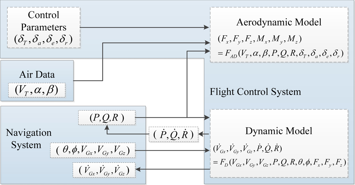
Figure 2. Relationship of Navigation System, Flight Control System and air data.

3.1. Equations of state

The state vector is defined as X = (V _T, α, β, P, Q, R, V _WN, V _WE)^T The state equation for (P, Q, R, V _WN, V _WE) can be obtained using Equations (8) and (4). The rest is the derivation of state equation of (V _T, α, β):

1. (1) Solve (V _Gx, V _Gy, V _Gz) with (V _T, α, β) and (V _WN, V _WE) through Equations (2) and (3).

2. (2) Solve $(\dot{V}_{Gx}, \dot{V}_{Gy}, \dot{V}_{Gz})$ with (V _Gx, V _Gy, V _Gz) through the aerodynamic model and the dynamic model, which are described in Equations (7) and (10).

3. (3) Obtain $(\dot{V}_{T}, \dot{\alpha}, \dot{\beta})$ with $(\dot{V}_{Gx}, \dot{V}_{Gy}, \dot{V}_{Gz})$ by differentiating Equation (2) as

(11)$$\left[\matrix{ \dot{V}\cr \dot{\alpha}\cr \dot{\beta} }\right] = \left[\matrix{ \cos \alpha \cos \beta & \sin\beta & \sin \alpha \cos\beta\cr {-\sin \alpha \over V_{t}\cos \beta} & 0 & {\cos\alpha \over V_{t}\cos\beta}\cr {-\cos\alpha\sin \beta \over V_{t}} & {\cos\beta \over V_{t}}& {-\sin \alpha \sin \beta \over V_{t}}\cr }\right] \left[\matrix{ \dot{U}\cr \dot{V}\cr \dot{W} }\right]$$

where $(\dot{U},\dot{V}, \dot{W})$ can be calculated through Equations (3) and (4) as follows

(12)$$\left[\matrix{ \dot{U}\cr \dot{V}\cr \dot{W} }\right] = \left[\matrix{ \dot{V}_{Gx},\cr \dot{V}_{Gy},\cr \dot{V}_{Gz} }\right] + \left[\matrix{ 0 & R & -Q\cr -R & 0 & P\cr Q & -P & 0}\right] \left[\matrix{ V_{WN}\cr V_{WE}\cr 0 }\right]$$

The state equation can be reorganised as

(13)$$\dot{\bf{X}} = f({\bf X}), {\bf U}_{1} + {\bf w}$$

where U₁ = (φ, θ, ϕ, δ _T, δ _a, δ _e, δ _r)^T is the control input, including the attitude angle from the NS and flight control parameters from the FCS and w is gauss white noise of the system with the variance matrix R.

3.2. Measurement equations

The measurement vector is defined as ${\bf Z} = (\hat{V}_{Gx},\hat{V}_{Gy}, \hat{V}_{Gz},\hat{P},\hat{Q},\hat{R})^{T}$, in which the variables are linear velocities and angular velocities from the NS. Usually real-time and high-accuracy navigation information can be obtained by fusing inertial navigation with GPS.

The measurement equations can be derived by Equation (3) as follows

(14)$${\bf Z} = h({\bf X}, {\bf U}_{2}) + {\bf v}$$

(15)$$h({\bf X}, {\bf U}_{2}) = \left[\matrix{ V_{T}\cos \alpha\cos\beta\cr V_{T}\sin\beta\cr V_{T}\sin\alpha \cos\beta }\right] + C^{B}_{N} \left[\matrix{ V_{WN}\cr V_{WE}\cr 0 }\right]$$

where U₂ = (φ, θ, ϕ)^T is the control input, v is the noise of measurements, Q is the variance matrix of v.

3.3. Extended Kalman filter

Considering the nonlinear character of the measurement equations, the Extended Kalman Filter (EKF) is applied to the state estimation problem of the dynamic model described by Equations (13) and (14). The nature of the EKF is minimum variance estimation following linearization and discretisation for nonlinear system through first-order Taylor approximation. Filter equations of the EKF are as follows:

(16)$$\left\{ \matrix{ \hat{{\bf X}}_{k+1/k} =\hat{{\bf X}}_{k} + f(\hat{{\bf X}}_{k}, {\bf U}_{1,k}) \cdot \Delta T\hfill\cr {\bf P}_{k+1/k} = {\bf \Phi}_{k}{\bf P}_{k}{\bf \Phi}^{T}_{k} + {\bf Q}\hfill\cr {\bf K}_{k+1} = {\bf P}_{k+1/k}{\bf H}^{T}_{k+1}({\bf H}_{k+1}{\bf P}_{k+1/k}{\bf H}^{T}_{k+1}+ {\bf R}^{-1})\hfill\cr \hat{{\bf X}}_{k+1}= \hat{{\bf X}}_{k+1/k} + {\bf K}_{k+1}\lcub {\bf Z}_{k+1} - h(\hat{{\bf X}}_{k+1/k}, {\bf U}_{2,k+1})\rcub \hfill\cr {\bf P}_{K+1} = ({\bf I}-{\bf K}_{k+1}{\bf H}_{k+1}){\bf P}_{k+1/k}({\bf I}-{\bf K}_{k+1}{\bf H}_{k+1})^{T}+{\bf K}_{k+1}{\bf RK}^{T}_{k+1} } \right.$$

where k is the current time, $\hat{{\bf X}}_{k}$ is the optimal state estimation with the variance matrix P_k, ΔT is the discrete time and Φ_k and H_k+1 are the Jacobian matrix of state equations and measurement equations respectively, which can be solved as

(17)$${\bf \Phi}_{k} = {\bf I} + {\partial f(\hat{{\bf X}}_{k}, {\bf U}_{1,k}) \over \partial \hat{{\bf X}}_{k}} \Delta T, {\bf H}_{k+1} = {\partial h(\hat{{\bf X}}_{k+1/k},{\bf U}_{2,k+1}) \over \partial \hat{{\bf X}}_{k+1/k}}$$

where I is the identity matrix.

3.4. Three-step Extended Kalman Filter

In the above model, we consider the wind speed as constant. However, this is only tenable for a short time. Using the EKF algorithm to solve the filter model cannot track the wind variation. For this problem, a three-step EKF is adopted. A Three-step Kalman Filter (TKF) algorithm is used to obtain estimation with uncertain input in a dynamic system. It considers the uncertain inputs as unknown variables. The estimation of these unknown variables is added to a traditional Kalman Filter. Gillijns and Moor (Reference Gillijns and Moor2007) proposed a TKF for discrete linear systems. According to the principle of EKF, the Three-step Extended Kalman Filter (TEKF) is derived through the linearization of nonlinear systems in this paper.

First, dividing the state vector into two parts, X = (X₁, X₂), in which X₁ = (V _T, α, β, P, Q, R)^T, X₂ = (V _WN, V _WE)^T · X₂. is considered as unknown variables. The linearized model is achieved and given in the following pattern (U₁, U₂ are hidden for convenience):

(18)$$\eqalign{ {\bf X}_{1,k+1} &= {\bf X}_{1,k} + f_{1}({\bf X}_{1,k}, {\bf X}_{2,k}) \cdot \Delta T + {\bf w}_{1} \cr {\bf Z}_{k} &= h({\bf X}_{1,k}, {\bf X}_{2,k}) + {\bf v} }$$

where w₁ is gauss white noise and Q₁ is the variance matrix of w₁. We denote the Jacobian matrices of the nonlinear state and measurement equations as follows:

(19)$$\eqalign{ {\bf A}_{k} &= {\bf I} + {\partial f_{1}(\hat{{\bf X}}_{1,k},\hat{{\bf X}}_{2,k}) \over \partial\hat{{\bf X}}_{1,k}} \Delta T, {\bf G}_{k}= {\bf I}+ {\partial f_{1}(\hat{{\bf X}}_{1,k},\hat{{\bf X}}_{2,k}) \over \partial\hat{{\bf X}}_{2,k}}\cdot \Delta T\cr {\bf C}_{k} &= {\partial h(\hat{{\bf X}}_{1,k},\hat{{\bf X}}_{2,k}) \over \partial\hat{{\bf X}}_{1,k}}, {\bf H}_{k}= {\partial f_{1}(\hat{{\bf X}}_{1,k},\hat{{\bf X}}_{2,k}) \over\partial\hat{{\bf X}}_{2,k}} }$$

Thus, the calculation procedure of TEKF is

1. (1) Estimation of unknown input:

   (20)$$\eqalign{ \tilde{{\bf R}}_{k} &= {\bf C}_{k}{\bf P}_{1,k/k-1}{\bf C}^{T}_{k} + {\bf R}\cr \hat{{\bf X}}_{2,k} &= ({\bf H}^{T}_{K}\tilde{{\bf R}}_{K}^{-1}{\bf H}_{k})^{-1}{\bf H}_{k}^{T}\tilde{{\bf R}}_{k}^{-1}({\bf Z}_{k}- h(\hat{{\bf X}}_{1,k/k-1}, 0))\cr {\bf P}_{2,k} &= ({\bf H}_{k}^{T}\tilde{{\bf R}}_{k}^{-1}{\bf H}_{k})^{-1} }$$

2. (2) Measurement update:

   (21)$$\eqalign{ {\bf K}_{k} &= {\bf P}_{1,k/k-1}{\bf C}_{k}^{T}\tilde{{\bf R}}_{k}^{-1}\cr \hat{{\bf X}}_{1,k} &= \hat{{\bf X}}_{1,k/k-1} + {\bf K}_{k}({\bf Z}_{k} -h(\hat{{\bf X}}_{1,k}, \hat{{\bf X}}_{2,k}))\cr {\bf P}_{1,k} &= {\bf P}_{1,k/k-1} - {\bf K}_{k}(\tilde{{\bf R}}_{k}- {\bf H}_{k}{\bf P}_{2,k}{\bf H}_{k}^{T}){\bf K}_{k}^{T}\cr {\bf P}_{12,k} &= -{\bf K}_{k}{\bf H}_{k}{\bf P}_{2,k} }$$

3. (3) Time update

   (22)$$\eqalign{ \hat{{\bf X}}_{1,k+1/k} &= \hat{{\bf X}}_{1,k} + f_{1}(\hat{{\bf X}}_{1,k}, \hat{{\bf X}}_{2,k}) \cdot \Delta T\cr {\bf P}_{1,k+1/k}&= \left[\matrix{{\bf A}_{k}\cr {\bf G}_{k}}\right]\left[\matrix{ {\bf P}_{1,k} & {\bf P}_{12,k}\cr {\bf P}^{T}_{12,k} & {\bf P}_{2,k}}\right]\left[\matrix{{\bf A}_{k}\cr {\bf G}_{k}}\right]+ {\bf Q}_{1} }$$

As shown in the above steps, the time and measurement updates of the state estimation adopt the form of the standard Kalman filter. The unknown input is isolated, and its value is replaced by an optimal estimate in the TEKF.

3.5. Initialised three-step extended Kalman filter

Lu et al. (Reference Lu, Eykeren, Kampen, Visser and Chu2016) points out that a TEKF is easily affected by the initial filtering error when applied to nonlinear filtering, subsequent experiments have verified this point. In this paper, an Initialised TEKF (ITEKF) algorithm is adopted. The EKF algorithm illustrated in Section 3.3 is used for filtering initialisation. When the filter is stabilised, the EKF algorithm can provide accurate initial estimates, and then switches to the TEKF algorithm. In this way, the accuracy of the TEKF algorithm can be ensured.

4.1. Simulation test procedure

For an air data estimation method based on information fusion of NS and FCS, the accuracy of estimated results is the key to verifying the feasibility and performance of the concept. The Generic Hypersonic Vehicle (GHV) aerodynamic model in Keshmiri and Colgren (Reference Keshmiri and Colgren2007) is used, and Equation (5) was used. After trimming the aircraft, we set the simulated vehicle flying under the three different conditions as shown in Table 1. Each flight lasts 30 seconds and the frequency of data was 10 Hz. We aimed to analyse the impact of measurement errors and a set of reference conditions shown in Table 2 was selected. In order to express the performance of the method proposed in this paper, the method in Lie and Egziabher (Reference Lie and Egziabher2013) was introduced and denoted as SADS2013 (Synthetic Air Data System 2013). The methods described in this paper are denoted as EKF, TEKF and ITEKF in accordance with the different filtering algorithms.

Table 1. Flight condition.

Table 2. Reference measurement errors (mean square deviation).

4.2. Simulation results without wind field change

To analyse the performance of the above algorithms without a wind field change, simulation was conducted under flight condition F1 and the measurement errors in Table 2. The results of these algorithms are shown in Figure 4 and Figure 5. Figure 4 shows the estimation error curves of airspeed, attack angle and sideslip angle. Figure 5 plots the estimation error curves of wind speed.

Figure 4. Estimation error curves of airspeed, attack angle and sideslip angle.

Figure 5. Estimation error curves of wind speed.

The above figures depict that SADS2013, EKF and ITEKF can quickly converge to the real values in the presence of an initial estimation error, and the convergence rate is about the same. TEKF is easily affected by the initial estimation error. As the first step of TEKF is to estimate the uncertain input or state, a large initial state error will lead to a large estimation error of uncertain input or state (wind speed). It can be seen from the wind estimation error curves that, the errors of wind speed estimation through TEKF appear larger than other methods at the initial time. Although the errors gradually decrease during the following process of filtering, the convergence speed is too slow to provide effective filtering estimation.

Compared to SADS2013, EKF and ITEKF are more accurate at estimating true air velocity and sideslip angle. The accuracy of attack angle estimation is about the same. The reason is that SADS2013 uses three-axis components of true airspeed as state variables and then calculates air data. A relatively small error of the three-axis components of true airspeed will generate a large error of true air velocity, sideslip angle and attack angle in this way. The method proposed in this paper uses true air velocity, sideslip angle and attack angle as the state. The effect of the three-axis true airspeed components estimation error on the air data estimation accuracy is reduced through the filter.

In order to make the conclusion more convincing, 100 repetitions of Monte Carlo experiments under F1~F3 flight conditions were conducted. The estimation errors’ statistical characteristics of SADS2013, EKF and ITEKF were calculated and are shown in Table 3. This shows that EKF and ITEKF are more accurate at estimating the true air velocity and sideslip angle than SADS2013, and the accuracy of the attack angle is about the same.

Table 3. Statistic characteristics of air data estimation errors.

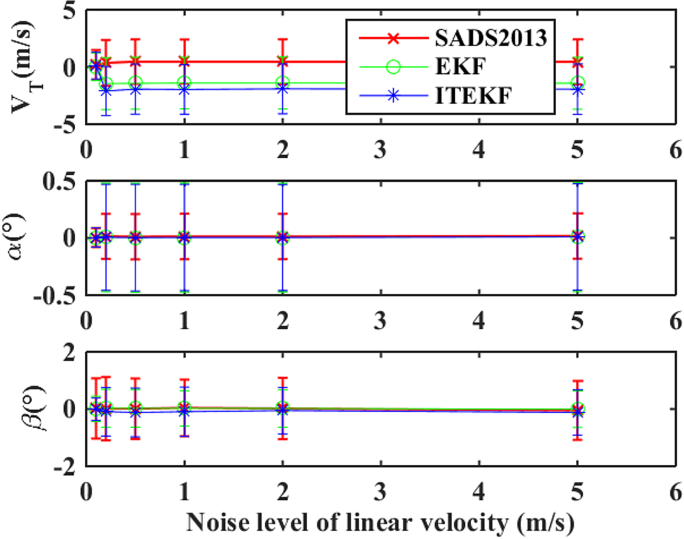
4.3. Sensitivity to the sensor noise and aerodynamic model error

Generally, the error of attitude is small, and the error in linear velocity is relatively large in the NS. Here the estimation errors under different linear velocity noise intensities are simulated and analysed. We set the noise intensity according to Table 2, 100 repetitions of Monte Carlo experiments were conducted under F1~F3 flight conditions. Then, we increased the linear velocity noise level and conducted more simulations in the same way. Simulation results are plotted in Figure 6. Results indicate that the filter can still achieve good estimation accuracy when the mean square deviation of the linear velocity measurement noise is increased to 5 m/s. This result is consistent with the filtering model. The influencing factors of the estimation of the state come from two parts: the aerodynamic and dynamic model in the state update and the linear and angular velocities in the measurement update. When the linear velocities contain large noises, the filter will calculate the state depending more on the state update and measurement update of angular velocities. Hence, the accuracy of state estimation can be ensured.

Figure 6. Estimation errors under different linear velocity noise levels.

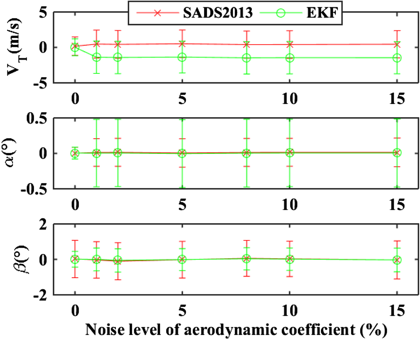
The aerodynamic model plays an indispensable role in the air data estimation. Through adding noise to the aerodynamic coefficients, the influence of an inaccurate aerodynamic model to the estimation performance was analysed. Noises at different percentages of the accurate aerodynamic coefficients were added separately. The mean and standard deviation of the errors are shown in Figure 7. The result shows that the filter can provide air data estimation with enough accuracy even if the error intensity of the aerodynamic coefficient is increased to 15%.

Figure 7. Estimation errors under different aerodynamic coefficient noise levels.

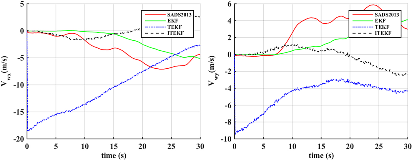
4.4. Simulation results with wind field change

The performance of the air data estimation methods with wind field change is tested in this section. The estimation errors of air data achieved through SADS2013, EKF, TEKF and ITEKF are shown in Figure 8. The wind speed estimation errors are shown in Figure 9, in which REFERENCE means the wind field set in the simulation. As shown in Figure 9, the X-component of wind speed is gradually changed from 10 s to 15 s, and the Y-component remains unchanged. SADS2013 and EKF have the trend to track the wind change; only ITEKF can track the wind change effectively and quickly; TEKF has a relatively larger initial deviation as a result of the initial estimation error, the subsequent estimation is highly influenced by the initial deviation. The conclusion can be drawn that ITEKF has the ability to track high-speed wind field change.

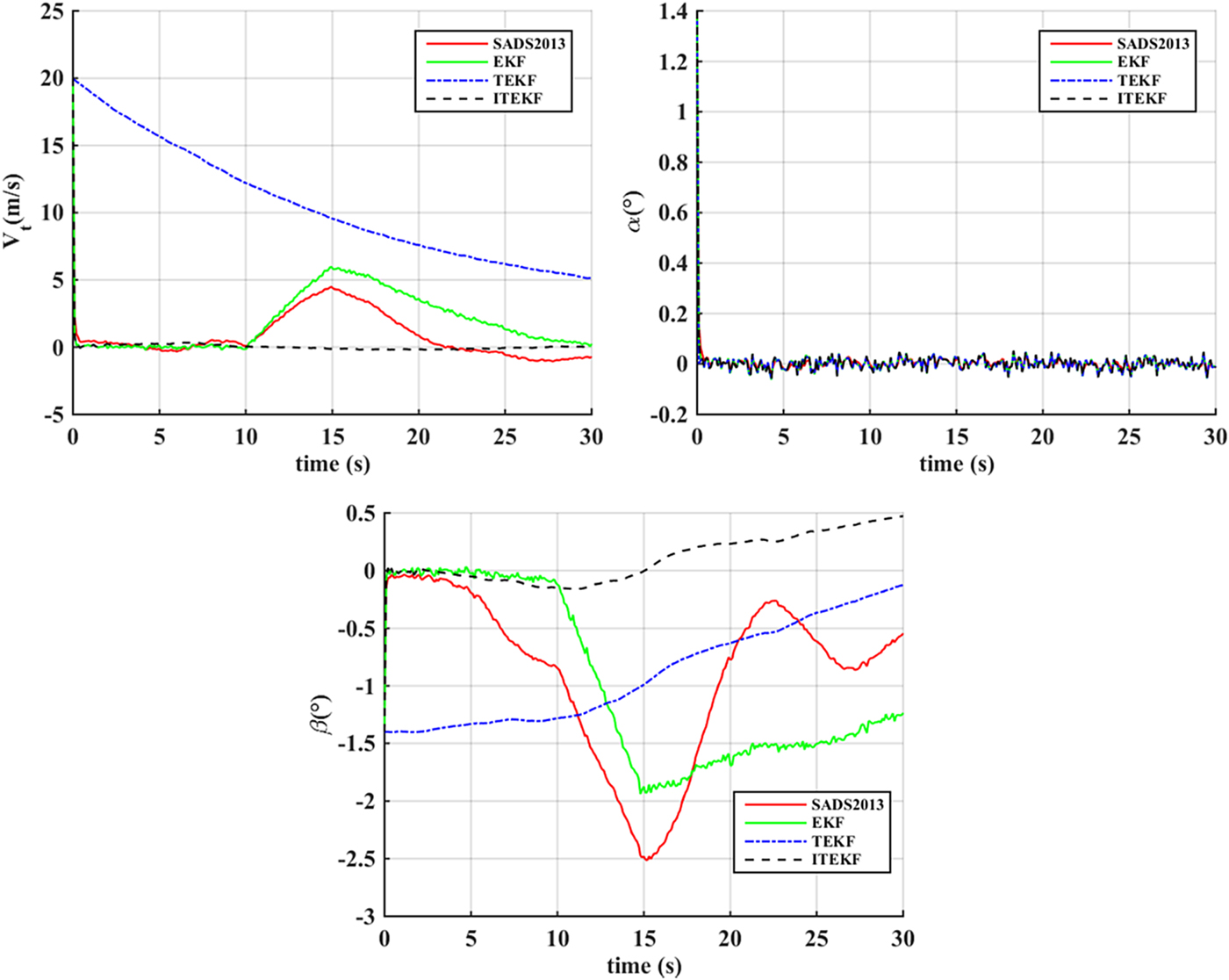
Figure 8. Air data estimation errors with variable wind field.

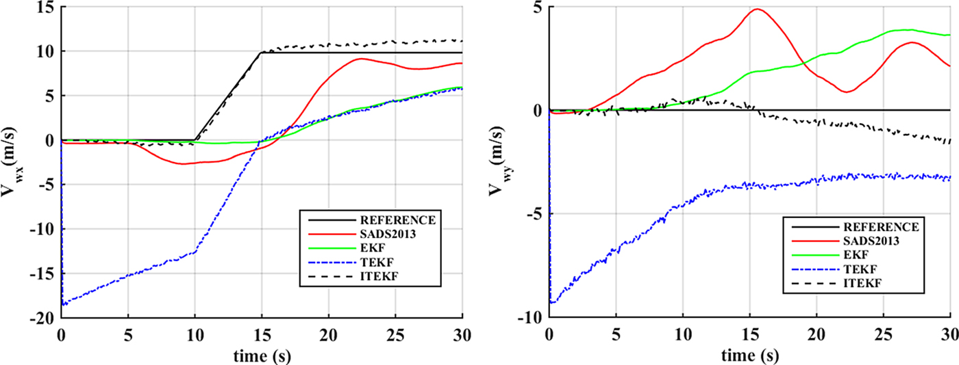
Figure 9. Estimation of wind speed with variable wind field.