

Introduction
After several decades of civil war and internal political conflict, economic growth took off in Argentina between 1870 and 1914. This period witnessed the longest and the highest period of growth in Argentine history and was based on the incorporation of productive factors (land, capital and labour) in a context of strong integration into international markets.Footnote 1 This process of economic development, with growth rates higher than those of the United States, transformed the country in many aspects and placed Argentina among the ten richest countries in the world.Footnote 2
After 1914 and, in particular, after the Great Depression of the 1930s, the direction of the country's macroeconomic policies and the pace and nature of its economic development changed dramatically: the level of openness was reduced in terms of both international trade and movement of productive factors, government intervention in the economy increased, and public expenditure and public deficits expanded along with inflation rates; growth rates of per capita income decreased until at least the 1950s.Footnote 3 In this context, domestic markets become more important, the traditional specialisation in agro-pastoral commodities weakened, and industrial production accelerated in absolute and relative terms.
We know very little about the relative economic performance of the different regions of the country in these periods. The first available consistent estimation of the GDP of the Argentine provinces was for 1953,Footnote 4 and it shows that the Capital Federal (the largest city in the country)Footnote 5 had the third highest GDP per capita in that year. Most of the other high-income districts were in Patagonia and had very low population densities: Tierra del Fuego was the first in terms of per capita income, Santa Cruz the second and Chubut and Río Negro the fourth and the fifth respectively. Historical evidence strongly suggests that this situation was relatively new: from colonial times a slow change took place in the relative economic importance of different regions within the current boundaries of Argentina. In pre-colonial times the mountainous north-west area was the most densely populated and, in the sixteenth century, the most affluent and important within a colonial system which linked it to the mining system in the Alto Perú. From the eighteenth century, the economic supremacy of Potosí and Lima started to be contested by the city of Buenos Aires and its growing involvement in the Atlantic trade.
After the wars of independence and during the period of the first globalisation in the second half of the nineteenth century the Pampa Húmeda (‘wet pampa’), with its comparative advantages in agro-pastoral activities, became economically more significant. In the last decades of the nineteenth century, some provincesFootnote 6 in Patagonia generated high per capita incomes in activities requiring intensive exploitation of natural resources, such as extensive cattle raising and mining. William Maloney and Felipe Valencia Caicedo confirm this long-run process of reversal in Argentina using correlations across provinces between income per capita today and population density – as a proxy for productivity – in pre-colonial times.Footnote 7 However, the timing and the causes of this reversal are not precise: was it caused by changes in colonial regulations in the eighteenth century? Or by Argentina's growing involvement in the Atlantic trade in the nineteenth century? Or, maybe, by dramatic change in the economic policies of the second third of the twentieth century? Although some evidence suggests that many important changes in the relative positions of the regions took place during the nineteenth century,Footnote 8 lack of comparable data makes impossible any precise assessment of the levels of regional development for any period before 1950.
In this paper, we present an estimation of the economic structure and the GDPs of the 14 provinces, the city of Buenos Aires and the ten national territories existing in 1914 in Argentina (25 districts). This year is particularly relevant because it marks the beginning of a significant change in the Argentine economy, from export-led to inward-looking state-led industrialisation that characterised the central decades of the twentieth century. Our results show that already in 1914, as in 1953, most of the population and the economic activity of the country were concentrated in the province and city of Buenos Aires. Regarding per capita income, we observe a firm persistence of the relative positions of the provinces in the ranking between 1914 and 1953; some districts in Patagonia (Tierra del Fuego and Santa Cruz), together with the Capital Federal, were the richest both in 1914 and 1953, while most of the provinces in the north of the country that were relatively poor in 1953 were already lagging at the beginning of the twentieth century. This consistence is remarkable given the different levels of openness, average growth, government intervention and, in general, development patterns prevailing between the two dates. In addition to these findings, we advance the hypothesis that the relative success of the high-income provinces was the result of, on the one hand, the continuation of a long process of growth of the city of Buenos Aires with agglomeration economies arising in the industrial and services sector and, on the other, exceptionally high labour productivity in Patagonia related to low population density and abundant natural resources that emerged well before the expansion of mining activities in the central decades of the twentieth century.
The rest of the paper is organised as follows: in the next section, we provide a short account of the theoretical reasons for economic persistence or reversal and discuss some of the relevant hypotheses and evidence for Latin America and Argentina. Then we present the available estimations of national GDP and some previous estimations of provincial income per capita for the period under consideration. The following two sections describe the methodology and data and present the results of our estimations for 1914 and the comparison with the available figures for 1953. Finally, we draw our conclusions. The on-line appendix provides some ancillary information.
Persistence, Reversal and Evolution of Argentina's Economy and its Regions in the Long Run
At least three different theoretical hypotheses can be proposed to explain regional growth and the patterns of persistence of or reversal in per capita incomes in Latin America and Argentina in the long run. Probably the most important is the distribution of locational fundamentals based on geographic characteristics, like latitude, access to the coast or abundance of natural resources, such as mining or fertile land. Where regions specialise in the production of goods intensive in natural resources, regional differences in productivity are shaped by the relative abundance of those natural resources. For instance, temperate regions with high-quality land will generate higher per capita income than those with worse land in tropical regions.Footnote 9 Of course, if purely geographic characteristics were the primary determinant of economic development, persistence would be the natural outcome.
Given that rich regions can decline and previously backward regions flourish, we can posit a modified geography hypothesis: geographic characteristics influence income per capita by interacting with a set of technological characteristics and relative prices. That is, a natural resource or a geographic advantage can be crucial for the production of a particular set of goods with a particular technology, but it can be irrelevant in a different context.Footnote 10 The commodity export boom in Latin America in the second half of the nineteenth century is an example of how certain regions exploited comparative advantages after a reduction in transportation costs and a change in relative prices.Footnote 11
The process of regional growth can also be affected by agglomeration economies arising when transportation costs, increasing returns and/or spill-overs induce producers to locate close to each other. If there are significant agglomeration economies at different points of a geographic space, the spatial distribution of income is shaped by the initial relative concentration of economic activity, population and market size. For instance, if there is an initial, possibly randomly located, cluster of producers with high productivity in a city and they are influenced by increasing returns, network effects and positive spill-overs, the potential new producers will choose to locate within or close to the cluster reinforcing the effect and, all other things being equal, increasing regional differences in income per capita.Footnote 12
Finally, different institutional frameworks have also been suggested as an explanation of the variability of income per capita across regions and its evolution across time. Daron Acemoglu and co-authors have proposed that a reversal in income per capita took place among the areas colonised in the fifteenth and the sixteenth centuries (Latin America among them). Before colonisation, incomes were positively correlated with population density, and high pre-colonial population density was linked to higher inequality and extractive institutions.Footnote 13 In the nineteenth century, when secure property rights were a pre-condition for growth, high-density regions experienced lower economic growth.Footnote 14
Many changes in the relative economic importance of regions in South America since colonial times are related to the expansion of and decline in mining activities around the city of Potosí. In the sixteenth century, a vast economically integrated space – from Ecuador to the north of Argentina and Chile – was articulated around the demand generated by the extraordinary economic and demographic expansion of the area surrounding the silver deposits of Potosí.Footnote 15 The north-west of Argentina, which specialised in the production of mules for transportation, food, and low-quality textiles, was more important and productive in this period than the marginal plains close to the River Plate. In the eighteenth century, Buenos Aires started gradually to gain importance as a commercial port within the expanding Atlantic trade and, afterwards, as the capital of the Viceroyalty of Río de la Plata.Footnote 16 Under the Spanish colonial system, imports within the Atlantic trade were limited and regulated, and the growing city of Buenos Aires increased demand for the production of the Interior (centre and north-west: Andean provinces of Mendoza, La Rioja and Catamarca; central provinces of Córdoba and Santiago del Estero; northern provinces of Tucumán, Salta and Jujuy) and started to compete with Potosí.Footnote 17 The wars of independence at the beginning of the nineteenth century resulted in the collapse of the economic networks based around Potosí, and the different provinces of contemporaneous Argentina engaged in a long period of civil wars between the Interior, the Litoral (mainly Santa Fe and Entre Ríos) and the province and city of Buenos Aires. The characteristics of trade policy (protectionism vs. free trade) and the administration of customs revenues were the major issues at stake within an economy that was increasingly oriented towards the Atlantic trade.Footnote 18
After the end of the civil wars, the economic evolution of Argentina until 1914 provides an archetypical example of rapid income growth based mainly on the exploitation of abundant fertile land and comparative advantages in the production of primary goods (wool, meat, cereals) for international markets. The expansion of available productive land in the south of the country was gradually complemented by an increase of labour supply through European migration (mainly Spaniards and Italians) and the expansion of productive capital through a significant inflow of foreign investment.
The east-central part of the country, sometimes known as the Pampa Húmeda (including mainly the provinces of Buenos Aires and Santa Fe, and some areas of Entre Ríos, Córdoba and La Pampa), was the epicentre of the expansion in livestock and cereal production. Technological changes in the meat refrigeration sector increased the relative value of cattle production and displaced sheep-raising to the south; after the Conquista del Desierto (‘Conquest of the Desert’, the military campaign to establish Argentine dominance over Patagonia) towards the end of the nineteenth century, sheep raising became the predominant economic activity in the large haciendas of Patagonia.Footnote 19 In this period, most of the provinces of the north languished because their artisanal manufacturing could not compete with cheaper imports.Footnote 20 The regional balance changed and the city of Buenos Aires consolidated its position as the most important urban centre of the country. Secondary and tertiary sectors nationwide also expanded before the First World War, but at a slower pace. The growth in manufactures was mainly concentrated in the sectors processing local raw materials for both exports (chilled meat and grain processing) and domestic consumption (food and beverages), with a high concentration in the city of Buenos Aires. In 1914 these sectors accounted for 42 per cent of total industrial production.
This model of economic development changed after the First World War and even more so after the worldwide recession of the 1930s. With the globalisation backlash, the international flow of goods, services and productive factors shrank. In Argentina, economic growth decelerated, and the country responded to the international context with increased levels of public intervention in the economy, higher tariffs, stimulation of the industrial sector and import substitution policies. In 1936 Argentina already had the second largest industrial sector in South America (in relative terms) encompassing not only the traditional sectors of food processing (cereal mills, meat processing plants) but also many sectors oriented to the internal market (textiles, metals, electrical).Footnote 21 The process of industrial growth, mainly located in the city of Buenos Aires and its industrial belt, went hand in hand with an acceleration in urbanisation and rural–urban migration, and reinforced the regional imbalance between Buenos Aires and the rest of the provinces that had started in the previous century.Footnote 22 The 1953 estimations, mentioned in the Introduction, suggest that in this year the city of Buenos Aires accounted for more than 19 per cent of the national population and that this district – together with some provinces in Patagonia (Tierra del Fuego, Santa Cruz and Chubut) – was the richest in per capita terms.
The only formal analysis of the historical process of the long-run changing regional patterns of development in Argentina is that by Maloney and Valencia Caicedo.Footnote 23 They explored the hypotheses of persistence and/or reversal of fortunes in the Americas at the subnational level in the long run (from the fifteenth to the twentieth century) and found that, within countries, persistence was the norm and that population density and per capita income in 2000, measured at the subnational unit, were strongly and robustly correlated with pre-colonial population density. However, Argentina is one of the two countries – the other is Chile – where significant reversals can be observed. The authors confirm that the north of Argentina, with relatively low per capita income today, was the most densely populated region before colonisation, while the wealthiest areas in Argentina in the twentieth century, in the centre and the south of the country, had low pre-colonial population density.Footnote 24 They suggest that the observed reversal can be mainly explained by the increasing importance of the city of Buenos Aires after the eighteenth century, the emergence of the previously low-population density region of the Pampa Húmeda as a significant exporter of agro-pastoral goods in the nineteenth century, and the specialisation of some Patagonian provinces in mineral activities in the second part of the twentieth century.
Previous Estimations of National and Provincial GDPs in Argentina
There are two principal independent estimations of the level of national GDP for 1914 in Argentina: the first was devised by the Comisión Económica para América Latina (Economic Commission for Latin America, CEPAL), which generated a GDP series for the period 1900–55, using information from a previous empirical work published by the Secretaría de Asuntos Económicos (Secretariat of Economic Affairs, SAE), and takes 1950 as the base year.Footnote 25 The second was proposed more recently by Roberto Cortés Conde, with data covering the period 1875–1935, using 1914 as the base year; it generates slightly higher growth rates for the period before 1930.Footnote 26 Later, both Orlando Ferreres and Gerardo della Paolera et al. generated new GDP series for this period, but these are, in one way or another, based on the CEPAL or Cortés Conde estimates.Footnote 27 The four series, although not exactly coincident, generate a quite similar picture of the trend of per capita income in Argentina in that period: vigorous growth between 1880 and 1914, a deceleration between 1914 and 1930.
At the provincial level, the first set of consistent estimations of economic activity was provided by the Consejo Federal de Inversiones (Federal Investment Council, CFI), an inter-provincial public institution created in 1959, which, in collaboration with the Instituto Torcuato di Tella (ITT), proposed the first official estimation of GDP in the provinces of Argentina for the years 1953, 1958 and 1959. The estimations are disaggregated and extremely detailed. They use the ‘value added by sector’ approach for 14 major sectors of economic activity in each province. The methodology to calculate the value added by sector, per province, is (1) direct calculation of the gross value of production minus intermediate consumption (raw materials, fuels, energy, etc.) and (2) distribution of national totals using an appropriate distributor. For instance, the values for the agricultural and livestock production sectors are estimated using the value added method while those for transport are calculated by distributing the total national figure.Footnote 28 Even though the methodology and sources are different from those we use in our study, the CFI–ITT make it clear that their estimation (‘gross geographical product at factor cost’)Footnote 29 is equivalent to the gross remuneration of all the productive factors used in the corresponding territory,Footnote 30 which is the approach we follow in our estimation. In this sense, the results seem to be comparable to ours.
We have almost nothing for any period before the middle of the twentieth century. Although there are some recent reconstructions of macroeconomic variables for some Argentine provinces in the nineteenth century, these are not strictly comparable because the methodology applied in each case was different.Footnote 31 This lack of reliable and consistent estimations of the level of economic activity in the provinces before the middle of the twentieth century has pushed some researchers to use imperfect proxies for testing their hypotheses. For instance, Lucas Llach used the level of public expenditure as a proxy for income per capita at the end of the nineteenth century, while Jorge Gelman relied on a very imperfect measure of wealth to derive inferences on regional inequality in the middle of that century.Footnote 32
Methodology and Data for Estimating Provincial GDPs in 1914
The most usual approach to calculate regional (or provincial) GDP in historical contexts is that proposed by Frank Geary and Tom Stark for the United Kingdom (which at the time included Ireland) between 1861 and 1911, based on the identification of a set of variables that can be used as predictors of the level of value added. In particular, they chose employment and sector-specific productivity, assuming that sector-specific wages capture such productivity.Footnote 33 There are many estimations of regional GDP in historical contexts based on the Geary and Stark methodology.Footnote 34
In this paper, we present an alternative approach to the calculation of several macroeconomic variables, including provincial GDP, for the 25 districts of Argentina in 1914; our methodology is based on the identity between GDP and the sum of the returns to productive factors (labour, land and capital). In order to calculate the value added in each province, we use the income approach to GDP and the identity between the sum of the added values and the sum of the returns to the productive factors. In particular, we will assume that the provincial GDP (Y) for each province will be:
 $$Y = \sum\limits_{i = 1}^N {L_i^{}} w_i + [ {r_AK_A + r_CK_C + r_IK_I + r_SK_S} ] + [ {q_AT_A + q_CT_C} ] + s_CC$$
The first term on the right-hand side of the equation is the remuneration to labour that is equal to the sum of all the wages paid to workers across the N different occupations. The second term in brackets encompasses the rents (r) paid to physical capital (K) in agriculture (A), livestock production (C) and in establishments in industry (I) and services (S). The third term, also in brackets, is the rent (q) paid to land (T) in agriculture and livestock production; and the last term is the flow of income generated by livestock (C). In this equation we allow the rate of return to differ between sectors.
Sources
The primary source on which we based our research was the Tercer Censo Nacional de la República Argentina (Third National Census of the Argentine Republic, TCN), taken on 1 June 1914, during the administration of Dr Roque Sáenz Peña.Footnote 35 Another important source of information was the book Riqueza y renta de la Argentina, by Alejandro Bunge;Footnote 36 it was crucial for allowing us to estimate the value added in agriculture and cattle production. We will provide more detail later about the way we used Bunge's information.
Information about wages came from several sources, mainly (but not exclusively) the Boletín (Bulletin) of the Departamento Nacional de Trabajo (National Department of Labour, DNT); these are described in detail below.Footnote 37
Labour Remuneration
To calculate labour remuneration, we used the TCN. This classified all the workers of each province in one of 436 occupations (so N in Equation (1) = 436) and gives information on the total number of male and female, Argentine and foreign workers in each category. These numbers are L i in Equation (1). One of the ‘occupations’ recorded by the TCN is ‘Varias y sin especificar’ (Various and unspecified), to which 1,793,661 individuals in Argentina were assigned; we assumed that this figure mainly captures the non-active population.Footnote 38 The other categories associated with the non-active population were students, the retired, beggars and ‘rentiers’, for whom we assumed zero income from labour. For categories related to entrepreneurial activities (like comerciantes, industriales, hacendados, etc.) we also have assumed zero income from labour (see the section on ‘Entrepreneurial profits’ in the on-line appendix for more details). In total, the active population in Argentina in 1914 was 3,121,091 individuals, and the active population made up 39.5 per cent of the total.
Information about wages comes mainly from:
(1) A report published by the DNT for 1912, citing wages for around 50 categories from 13 provinces (Buenos Aires, Catamarca, Córdoba, Corrientes, Entre Ríos, Jujuy, La Rioja, Mendoza, Salta, San Juan, San Luis, Santa Fe and Tucumán).Footnote 39 The province of Santiago del Estero and the national territories (Los Andes, in the north-west; Chaco, Formosa, Misiones in the north-east; La Pampa in the centre; Neuquén, Chubut, Río Negro, Santa Cruz and Tierra del Fuego in the south) were excluded from the report. In general, the most significant categories in the provinces with the largest populations were included; the active population of these provinces was 2,883,656 while that of the excluded regions was only 237,435.
(2) For Buenos Aires, we also used wages information for another 90 categories presented in the Anuario Estadístico (Statistical Yearbook) published by the DNT in 1916, with information for 1914.Footnote 40
(3) A DNT report with wages for some categories in the national territories of Misiones and La Pampa.Footnote 41
From the information above we assigned wages to 1,628,918 individuals in the 13 provinces listed in (1) above and two national territories (La Pampa y Misiones). This represented 52.19 per cent of the active population in the country.
We do not have direct information for the provinces of Santiago del Estero, Chaco, Formosa, Neuquén, Chubut, Santa Cruz, Tierra del Fuego and Los Andes. The total active population in these provinces was only 182,321 individuals (5.8 per cent of the total active population in the country). For these provinces, we assigned wages similar to those in the closest and/or the most similar province in geographic terms for which we had information. In particular:
(4) We have used wages from Catamarca (the province of the north-west with the lowest average salary) for Santiago del Estero and Los Andes.Footnote 42
(5) For the five Territorios Nacionales in Patagonia (Neuquén, Chubut, Río Negro, Santa Cruz and Tierra del Fuego) we used a proportion of the wages in La Pampa. This proportion is from a DNT report for 1907 with reports of wages for labourers (peones) in La Pampa and four of the national territories (excluding Neuquén).Footnote 43 The details of the process are in the on-line appendix.
(6) For San Luis, we used wages similar to those in Córdoba. (Wages for the categories of casual labourer (peón–jornalero), carpenter, tinsmith, building worker and blacksmith (the most significant categories in general) in the two provinces were very similar.)Footnote 44
To impute a wage to the remaining categories in all the provinces we classified them in four groups of workers according to the skill required and extrapolated known wages of workers in each category to the workers with missing wages in the same category.Footnote 45 The details of this process and other methodological decisions to complete the data on wages and workers are presented in the on-line appendix.
Capital Used in Industry and Services
We include in the secondary (industrial) sector all activities associated with the transformation of food and raw materials through industrial processes and other activities, like building, energy, iron and steel making, textiles, etc. The tertiary sector includes commercial activities, transportation, financial services, insurance, education, etc.Footnote 46
The capital stock for each of the sectors mentioned in the previous paragraph was obtained directly from the TCN volumes relating to industry and commerce. The capital stock used in industry included both fixed capital (building, land, machinery and implements) and working capital (all the material used in the process of production).Footnote 47 The branches of activity included in the TCN were: general industries, mills, salting factories, wine and beer factories, sugar mills, distilleries, gas factories and electric light plants. In order to account for differences between sums declared for individual assets and total capital investment, one of the TCN’s commentators stated: ‘Under no circumstances should the capital sums imputed to industrial production be considered exaggerated; on the contrary, they should be considered to be under-reported by 30 per cent.’Footnote 48 With this statement in mind we increased total capital in the secondary sector by 43 per cent.Footnote 49
In the services sector the underestimation of the capital stock for food, clothes and toiletries, teaching, buildingFootnote 50 and transport seems to be even more significant than in the case of industry, and the TCN figures should be increased by 100 per cent.Footnote 51 The TCN’s commentator said: ‘The same problems as those observed in the 1895 Census, i.e. an under-declaration of capital, which the Census estimated at 50 per cent, must have existed in 1914, because always, and everywhere, even in the countries most used to this type of research, declared capital, both in trade and in industry, is lower than actual.’Footnote 52 We also considered capital stock in railways, tramways, ports, public utilities, printing and hospitals.Footnote 53
To calculate r IKI + r SKS, which is the contribution of capital in secondary and tertiary sectors to total output, we used a rate of return to capital of 8 per cent, following the TCN’s ‘Considerations on the Results of the Livestock Census’.Footnote 54
Land and Capital in the Primary Sector
Regarding income from agriculture and pastoral activities, the information used in this paper comes mainly from TCN, Vols. 5–6 and Bunge, Riqueza y renta. To get the value added generated by land in agriculture, we applied TCN data on the quantity of land used in agriculture and yearly rents (in pesos, AR$) in each province.Footnote 55 In this way, the value added by land in agriculture would be q ATA, where q A is the yearly rent and T A is the land used in agriculture.
In order to estimate the value added by other productive factors (in this case, capital) we used information from the TCN on the value of fixed capital (stables, fences etc.) and machinery and implements. Given that the TCN did not discriminate between capital in agriculture and capital in pastoral activities, we relied on Bunge, who claimed that one-third of the fixed capital was used in agriculture and two-thirds in livestock production;Footnote 56 regarding machinery and implements, we assumed that 100 per cent was used in agriculture.Footnote 57 The value of capital in agriculture was combined with a rate of return of 8 per cent; the value added by this productive factor was obtained with the formula r AKA.
Bunge suggested that the yearly value added in livestock production was equal to 15 per cent of the value of the livestock.Footnote 58 Given that the TCN provided the total value of the livestock for each province,Footnote 59 it was possible to calculate the value added by livestock production in each province. However, this would not be equal to r CKC + q CTC + s CC in Equation (1) because the number provided by Bunge included the return to labour. Unfortunately, it was not possible to discount the value added by labour in livestock production (obtained from our estimation of the value added by labour and described in an earlier sub-section) because there were many occupations in the TCN classification that included workers from both agriculture and livestock production.Footnote 60 Bunge made it clear that, once the return to capital and land was discounted, one-third of the remaining return went to labour and two-thirds was the economic return of livestock.Footnote 61 So, by calculating the value added of land and capital, it was possible to arrive at the combined value added by both labour and livestock as a residual and then to use the one-third/two-thirds shares suggested by Bunge to obtain the return to each.
The total return to land in cattle production (q CTC) was obtained using the value of land rents per hectare (in pesos, AR$) and the quantity of land. The quantity of land was obtained from the total quantity of animals of each kind in each provinceFootnote 62 and technical equivalence coefficients for the ratio of livestock and land.Footnote 63
The value added by capital was calculated using the total value of capital in agro-pastoral establishments and, as we mentioned before, following Bunge (two-thirds share to pastoral establishments). The rate of return of this capital, according to Bunge, was 4 per cent.Footnote 64
From the two previous paragraphs, we obtained q CTC and r CKC. The value s CC was obtained by subtracting these two values from the total value added in agriculture and multiplying the result by two-thirds (in order to discount the value added by labour).
Results
The Relative Affluence of the Provinces in 1914
Combining all the information above we obtained a total national GDP of AR$4.2 billion (1914 values), more than half of which was contributed by the Capital Federal and Buenos Aires (Table 1); Santa Fe represented 12.7 per cent, Córdoba 8.6 per cent and Entre Ríos 4.2 per cent, all of them in the centre region of the country. Providing a minor contribution were the provinces of Tucumán in the north (3 per cent) and Mendoza in the west (2.9 per cent).
Table 1. Argentina: Regional Aggregate and Per Capita GDP in 1914 and 1953

Notes: a Current 1914 thousands of AR$.
b Current 1914 AR$.
c Current 1953 AR$.
d Totals are rounded.
Sources: Aggregate GDP and per capita GDP for the year 1914: authors’ elaboration (see text).
Per capita GDP and population for the year 1953: CFI–ITT, Relevamiento de la estructura regional, Vol. 2, p. 159 (population), p. 205 (GDP data).
Population density: authors’ estimation based on population data from (1914) TCN, Vol. 1, p. 58 and (1960) CFI–ITT, Relevamiento de la estructura regional, Vol. 2, p. 159 and land area: from (1914) TCN, Vol. 1, p. 202 and (1960) Dirección Nacional de Estadísticas y Censos, Censo Nacional de Población 1960, Vol. 1 (Buenos Aires: Dirección Nacional de Estadística y Censos, 1960), p. 2.
The emergence of the conglomerate of the Capital Federal and Buenos Aires as the main centre of the economic development in Argentina was complete by 1914. The regions of the Interior, allegedly more important in the colonial period, had lost much of their relative affluence by the beginning of the twentieth century. While the province of Buenos Aires had the largest areas of agricultural production and the most extensive cattle stocks in the country, the Capital Federal accounted for 31 per cent of total capital in manufacturing and 50 per cent of total capital in commerce.
Our approach generates an estimation of the national GDP per capita of AR$530, relatively close to the figure of AR$572 estimated by Cortés Conde.Footnote 65 This correspondence is remarkable given that the methodology used for our estimation is very different from that used in previous approaches.Footnote 66
To calculate the share of each economic sector (primary, secondary and tertiary) in the GDP we need to define the economic sector of each factor of production. This is trivial for land and livestock which are, by definition, in the primary sector. When providing the value of capital, the TCN was very specific as to whether it belonged to the primary, secondary or tertiary sectors. In the case of labour, the TCN classified the list of occupational categories into 16 groups which, in most cases, could be easily assigned to a specific economic sector. The notable exceptions were the categories jornaleros and peones, which were in the group ‘General designations without indication of a specific profession’. To solve this problem, we assumed that the total amount of wages in each sector was proportional to the relative value added generated by capital, land and livestock in the sector.
With this methodology, we were able to apportion the GDP of each province to the primary, secondary and tertiary sectors (Table 2). At the national level, the relative size of each sector is quite similar to that obtained by Cortés Conde,Footnote 67 with 33.9 per cent of value added in the primary sector, 28.4 per cent in the secondary and 37.7 per cent in trade and services. Most of the capital in industry was in the Capital Federal and Buenos Aires (31 and 26 per cent of the total national value of capital in industry, respectively); the most important sub-sectors within the industrial sector were food processing and energy production. Food processing accounted for 39 per cent of the total capital in the industrial sector in Buenos Aires and 14 per cent in the Capital Federal; in Tucumán, Mendoza, San Juan and Jujuy the capital invested in the food processing sub-sector was more than 70 per cent of the capital in the secondary sector.Footnote 68 The provinces with the largest secondary sectors were Tucumán and Mendoza (Table 2). In the case of Tucumán the size of the industrial sector was linked to sugar mills, and in Mendoza the most important industry was wine production.
Table 2. Argentina: Sector Distribution of GDP by Region, 1914

Note: Percentages are rounded.
Source: Authors’ elaboration. See text.
The provinces of the Pampa Húmeda (Buenos Aires, Santa Fe, Córdoba and Entre Ríos), with undeniable comparative advantages in cereal and livestock production, had relatively large primary sectors, as did most of the provinces in Patagonia (Tierra del Fuego, Santa Cruz, Río Negro). Regarding the relative importance of the tertiary sector, the Capital Federal stands out with a value added of almost 62 per cent in that sector.
The top positions in the ranking of per capita GDP were occupied by Santa Cruz, Tierra del Fuego, the Capital Federal, La Pampa, Santa Fe and Buenos Aires (see Table 1). The poorest provinces were Santiago del Estero, Misiones, Catamarca, Corrientes and Salta. By 1914, the north of the country was already relatively backward.
Most of the descriptions of Argentina at the beginning of the twentieth century emphasised the comparative advantage of the cereal-growing and cattle-raising area in the centre of the country, corresponding approximately to the provinces of Buenos Aires, Santa Fe and parts of Córdoba, Entre Ríos and La Pampa. In this context, the relative positions in our results of some provinces like Santa Cruz and Tierra del Fuego in Patagonia are surprising. All the provinces in Patagonia (and Formosa in the north-east) have very low population density (see Table 1) and a comparatively large quantity of livestock per capita, and this explains the high income per capita in Santa Cruz and Tierra del Fuego. In Santa Cruz, income generated only by cattle-raising (excluding wages) was AR$330.67 per capita, which was higher than the total GDP per capita in provinces like Catamarca and Santiago del Estero. In Tierra del Fuego, income generated from cattle-raising (again excluding wages) was AR$235.57, while the national average was AR$61.90 per capita and in Buenos Aires it was AR$112.75 per capita.
A comparison of the sectoral compositions of the more affluent districts can shed light on the debate about the reasons for the regional disparity in relative incomes. Provinces like Buenos Aires, Santa Fe and La Pampa on the one hand, and Santa Cruz and Tierra del Fuego on the other, derived more than 45 per cent of their GDP from the primary sector: the first group of provinces belongs to the Pampa Húmeda, the traditional area of cereal production and cattle and sheep raising; the second group of provinces is part of Patagonia, whose value added in the primary sector was related not to agricultural production but rather to the specialisation in sheep raising that took place after the Conquista del Desierto.Footnote 69Although the two groups had different specialisation profiles, high incomes in all these provinces were related in one way or another with a natural comparative advantage arising from land abundance. In Santa Cruz and Tierra del Fuego, mineral activities became important when oil deposits were discovered in the 1940s; oil extraction started in Comodoro Rivadavia (province of Chubut) in 1907, but was negligible until the beginning of the First World War.
The Capital Federal (with the third-highest income per capita and responsible for almost 26 per cent of the total GDP of the country) exhibited an entirely different pattern. This region was an almost purely urban district in which the primary sector accounted for less than 1 per cent of GDP and in which the tertiary sector, where economies of scale were more feasible, produced more than 60 per cent of the value added.
The Evolution of the Regional Pattern of Income per Capita in the First Half of the Twentieth Century
Our estimation not only provides the essential information for understanding the relative affluence of the provinces in 1914, but also opens up the possibility of comparing the 1914 regional distribution of income with that in 1953 and of analysing the regional dimension of the economic changes that took place in Argentina in the first half of the twentieth century. According to the estimations by CFI–ITT, the two districts with the highest GDP per capita in 1953 were Tierra del Fuego and Santa Cruz.Footnote 70 The Capital Federal was in third position, and Chubut and Río Negro in fourth and the fifth positions, respectively; the provinces of Buenos Aires, La Pampa and Santa Fe, representative of the traditional cereal-growing and pastoral production, occupied the sixth, seventh and ninth positions.
Figure 1 shows the relationship between the logs of income per capita of provinces in 1914 estimated in this paper and the log of income per capita in 1953 according to the CFI–ITT. Despite almost 40 years of profound changes in economic structure and policies, the association is remarkable. A simple linear regression between the two variables shows that the log of GDP in 1914 can explain almost 78 per cent of the variance of the log of GDP in 1953, and the elasticity of GDP in 1953 to changes in GDP in 1914 is very close to 1.Footnote 71 In Argentina in the first half of the twentieth century, we observe neither reversal nor convergence but, rather, clear persistence. The long process of reversal since colonial times suggested by the historical accounts seems to have been completed by the beginning of the twentieth century, when the city of Buenos Aires and some provinces in Patagonia were already the wealthiest districts in the country.Footnote 72
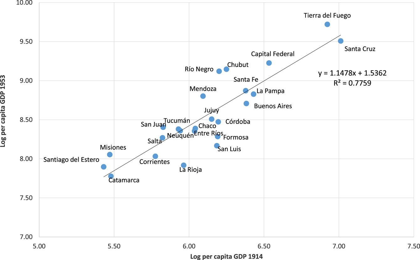
Figure 1. Argentine Provinces: Logs of Income per Capita, 1914 and 1953
A closer inspection of the sectoral composition of the GDP of the three most affluent districts in 1914 and 1953 helps to highlight the different processes involved. In the Capital Federal, in 1953, the primary sector made almost no contribution to GDP (it provided just 0.1 per cent, from fisheries): the secondary sector (manufacturing and building) accounted for 35.8 per cent and the tertiary sector for the remaining 64.1 per cent (mainly trade, government and other services);Footnote 73 this structure was very similar to that observed in 1914. The economic structure of the province of Buenos Aires changed substantially in the period under consideration: the primary sector accounted for only 22.4 per cent in 1953 (less than half of the contribution 40 years earlier) and between 1914 and 1953 its industrial sector expanded by almost ten percentage points until reaching 31.5 per cent of GDP. Most of the industrial sector was located in the area very close to the boundaries of the city of Buenos Aires, suggesting a process of spill-over of the industrial activity from that district.Footnote 74 Following the process of concentration of the secondary sector in the Capital Federal and its hinterland in the province of Buenos Aires, 75.2 per cent of the national production in manufacturing in 1953 was located in those two districts. At the same time, 39.9 per cent of the value added in the tertiary sector in Argentina was produced in the city of Buenos Aires. The economies of agglomeration and the expansion of the secondary and tertiary sectors already present in 1914 in the Capital Federal not only persisted in that district but even expanded to the province of Buenos Aires and changed its economic structure.
The province of Santa Cruz (the second richest in both 1914 and 1953) seems to provide a clear example of the importance of the abundance of natural resources: in 1953, 46.3 per cent of the provincial GDP came from livestock production and the second most important sector was mining with 11.3 per cent.Footnote 75 In 1914 the primary sector accounted for 50.7 per cent of provincial GDP (Table 2). In 1914, the primary sector in Tierra del Fuego accounted for 46.8 per cent of GDP and most of that came from pastoral production; in 1953, 28.0 per cent of provincial GDP was due to livestock production, and 12.3 per cent came from the fishing sector.Footnote 76
The sector composition of the GDP in the more affluent provinces suggests that their processes of growth did not share a common underlying rationale. In the Capital Federal and some areas in the province of Buenos Aires, most of the growth took place in the secondary and tertiary sectors, where the emergence of agglomeration economies was more feasible. At the same time, high levels of income per capita in Tierra del Fuego and Santa Cruz – in both 1914 and 1953 – suggest that natural resources (firstly abundant land for sheep raising and then mineral resources) were enough for the retention of an advantageous situation under very different economic conditions.
Conclusions
The present-day regional distribution of income in Argentina seems to be the result of a long process of reversal. While in the first part of the colonial period the northern part of the country was the most important and the richest, in the second half of the twentieth century the city of Buenos Aires and some provinces in Patagonia had the highest income per capita.
Our evidence shows that these relative positions were already defined in 1914 and that the first half of the twentieth century was characterised by the persistence of relative positions of income per capita; the long-run process of reversal had already been completed by the beginning of the twentieth century.
Within the set of the leading districts in both 1914 and 1953 the productive profiles differ: the provinces of Patagonia, incorporated into the national market only in the last decades of the nineteenth century, at the beginning based their growth on extensive sheep raising and, after the 1930s, on oil production. The very high incomes per capita in 1914 in Patagonia were related to land abundance, low population density and very high labour productivity. In this sense, our results show that the role of these provinces in the process of reversal was related not only to mineral resources after 1930 (as suggested by Maloney and Valencia Caicedo)Footnote 77 but also to high pastoral production in the first decades of the twentieth century.
The increasing importance of the city of Buenos Aires, in the long run, was the result of, first, the expansion of Atlantic trade in the eighteenth century; then its consolidation as the prime commercial and administrative centre in the nineteenth century and, finally, as shown in our estimations, by the concentration of most of the industrial and services activities in the period of import substitution in the central decades of the twentieth century. Our results indicate that the leading role of the city of Buenos Aires was very well established by the first decades of the twentieth century; in 1914 it contributed more than 25 per cent of total national GDP and had the third highest GDP per capita. Most of the value added in the city of Buenos Aires was generated in manufacturing and services both in 1914 and 1953, suggesting that agglomeration effects played an essential role in this district. Disaggregated information for 1953 also suggests that there were some spill-overs into the areas in the province of Buenos Aires located close to its boundary, producing an expansion in the manufacturing sector in that province.
The provinces in the north of Argentina exhibited the downside of this persistence: they were already comparatively poor in 1914 and continued to lag behind the other regions of the country during the twentieth century. Santiago and Catamarca in the north-west and Misiones and Corrientes in the north-east were in the bottom six positions in both 1914 and 1953.
Regional imbalance in the processes of economic growth and development is a central concern for economic historians, economists and policymakers. Regional inequality seems to be insensitive to changes in macroeconomic strategies, cohesion policies and targeted interventions. In the very long run, Argentina experienced a change in the relative affluence of the regions. However, marked structural change and substantial modifications in the strategic and social priorities of the policymakers, in the role of the public sector, and in the level of integration into the global markets of the first half of the twentieth century did not have a noticeable impact on the geographic pattern of economic development of the country. The high income per capita of some districts in Patagonia and the city of Buenos Aires and the low income per capita of most provinces in the north of the country has been the dominant pattern at least since 1914.
Supplementary material
The supplementary material for this article can be found at https://doi.org/10.1017/S0022216X19001299.


