1. Introduction
How does institutional change affect economic growth? This paper explores a new hand-collected data set and within country variation over extremely long-time horizons using an uncommon econometric framework to assess the effect of political instability on the growth rate of gross domestic product (GDP). We focus on both direct changes in formal political institutions and on potential indirect changes through political instability.
Institutional change can occur through changes in formal or through changes in informal political institutions. The latter includes for example events of socio-political unrest – mass violence such as assassinations, revolutions and riots, and the former includes events such as government terminations and electoral surprises. In other words, formal political instability indicators are the result of the competition between different political institutions or factions whereas the informal political instability measures have no appropriate representation within such channels.
Within a power-ARCH (PARCH) framework and using annual time series data for Brazil covering the period from 1870 to 2003, the aim of this paper is to put forward answers to the following questions. What is the relationship between the instability of a country's key political institutions, economic growth and volatility? Are the effects of these changes in institutions direct (on economic growth) or indirect (via the conditional volatility of growth)? Does the intensity and sign of these impacts vary over time? Does the intensity of these effects vary with respect to short- versus long-run considerations? Is the intensity of these effects constant across the different eras or phases of Brazilian economic history (in other words, are they independent from the main structural breaks we estimate)?
This paper tries to contribute to the existing literature by examining whether the instability of a country's key political institutions affects output growth. This approach is original and valuable because: (a) we study only one individual country over a very long period of time with annual frequency data. Most previous research assesses political instability from a cross-country perspective (Barro, Reference Barro1991; Fosu, Reference Fosu1992; Levine and Renelt, Reference Levine and Renelt1992 and so on) whereas others focus on shorter periods (Campante, Reference Campante2009), (b) we use the economic history literature to guide our choice of potential reasons behind the performance of the Brazilian economy over a very large time window, (c) we construct and use new, unique, hand-collected data on political institutions in Brazil going back as far as 1870 (the existing data start in 1919 so we independently constructed whole new series from 1870 to 1939, using the overlapping 20 years to assess the reliability of our new data), and (d) we choose an econometric methodology that has been seldom used in the empirical growth literature despite the fact that it easily allows us to contrast the direct to the indirect (i.e. via the volatility channel) effects of each of our candidate reasons, sort out the short- from the long-run impacts, and distil the consequences of accounting for important structural breaks on the robustness of our key results.
Another important, albeit more technical, benefit of our choice of econometric framework is that it helps to shed light on an important puzzle on the relationship between output growth and its volatility. For example, although Ramey and Ramey (Reference Ramey and Ramey1995) show that growth rates are adversely affected by volatility, Grier and Tullock (Reference Grier and Tullock1989) argue that larger standard deviations of growth rates are associated with larger mean rates. The majority of ARCH papers examining the growth-volatility link are restricted to these two key variables. That is, they seldom assess whether the effects of the presence of other variables affect the relation and, on the rare occasions that happens, it is usually inflation and its volatility that comes into play. For reviews of this literature see Fountas and Karanasos (Reference Fountas and Karanasos2007) and Gillman and Kejak (Reference Gillman and Kejak2005).
The Brazilian case is particularly interesting to study the relationship between the instability of political institutions and economic performance. Brazil is relevant because of its size (both in terms of populations and output), its hegemonic role in South America and its relatively important role globally. It is also important because despite the reputation of having a relatively peaceful history, this is a country that exhibits a rich variety of types of instability of political institutions (indeed of all the formal and informal types one can find in large cross-sections of countries) under considerable variation of contexts (empire and republic as well as over varying degrees of democracy and autocracy), over the very long time window we consider.
Our main results can be organised in terms of different types of effects. We discuss direct (on mean economic growth), indirect (via volatility), dynamic (short- and long-run) and structural break effects. As for the direct effects of institutional change on economic growth, we find evidence for negative direct influences on real GDP growth from both the informal political instabilities (i.e. assassinations, coups and revolutions) and formal political instabilities (i.e. legislative effectiveness and number of cabinet changes). Equally importantly, we find that almost all of our political instability indicators have strong negative impacts on the output growth in the short run. As for indirect (via volatility) effects, we find strong volatility-decreasing effects from both formal and informal political instability indicators.
Our investigation of the dynamic effects shows important differences in terms of the short- and long-run behaviour of our key variables: almost all political factors affect growth negatively in the short-run but the evidence for the long-run is much weaker. Importantly, however, the negative impact of assassinations, coups, revolutions together with legislative effectiveness and cabinet changes remains strong in the long-run. Finally, we tried to adjust all the above results to the possibility of the presence of structural breaks. This is an important exercise given the long-term nature of our data. We find that our basic results are confirmed once we take structural breaks into account. It is also noteworthy that the contemporaneous direct effects on growth of our main explanatory variables (i.e. anti-government demonstrations and assassinations) are stronger before the structural breaks, whereas the indirect effects are weaker after accounting for these breaks. Hence and in summary, over the whole range of results (negative direct/indirect, short- and long-run impact on economic growth) the most robust we find are those obtained for assassinations, number of coups, legislative effectiveness and cabinet changes.
The intricate relationship between institutions and political instability has been examined in detail by many authors. In a seminal paper, using a cross section framework, Barro (Reference Barro1991) finds that assassinations, number of coups and revolutions have negative effects on economic growth. Campos and Nugent (Reference Campos and Nugent2002) confirm this result by using panel data analysis but find that this negative impact (on growth) is mostly driven by sub-Saharan African countries. Easterly and Rebelo (Reference Easterly and Rebelo1993) suggest that assassinations and war casualties have no significant effect on growth, whereas Benhabib and Spiegel (Reference Benhabib and Spiegel1997) and Sala-i-Martin (Reference Sala-i-Martin1997) empirically support this argument. Knack and Keefer (Reference Knack and Keefer1995) compared more direct measures of institutional environment (such as the security of property rights and the Gastil indicators of political freedoms and civil liberties) with instability proxies utilised by Barro (Reference Barro1991). Asteriou and Price (Reference Asteriou and Price2001) examine the influence of political instability on UK economic growth and find that political instability affects growth negatively whereas it has a positive impact on its uncertainty. Spruk (Reference Spruk2016a) examined the impact of de jure and de facto political institutions on the long-run economic growth for a large panel of countries. The empirical evidence suggests that societies with more extractive political institutions in Latin America experienced slower long-run economic growth and failed to converge with the West.
An important issue regards the channels through which political instability is expected to influence growth. It might be expected that instability will make property rights less secure and transaction costs too high, the rule of law weak and state capacity too thin to support sustained growth episodes. Furthermore, political instability is likely to affect the behaviour of both voters as well as monetary and fiscal authorities thus influencing economic decisions and output.
For example, Torstensson (Reference Torstensson1994) argues that many developing countries lack secure private property rights and that arbitrary seizures of property slow down economic growth. Kovač and Spruk (Reference Kovač and Spruk2016) quantify the impact of increasing transaction costs on cross-country economic growth and find a significant negative effect. Weingast (Reference Weingast1997) studies the role of political officials' respect for the political and economic rights of citizens supporting democratic stability and the rule of law. Acemoglu et al. (Reference Acemoglu, García-Jimeno and Robinson2015) study the direct and spillover effects of local state capacity in Colombia and find that the existence of central and local states with the ability to impose law and order is vital for economic development. Finally, Carmignani (Reference Carmignani2003) argues that political instability through phenomena of social unrest, volatility of policymakers, fragmentation of the decision-making process and electoral uncertainty is expected to be a substantial determinant of economic output.
The paper is organised as follows. Section 2 sets the historical context for the paper by documenting Brazilian political history. Section 3 describes the data. Section 4 provides details and justification for our econometric methodology. Section 5 presents our econometric results. Section 6 concludes and suggests directions for future research.Footnote 1
2. Economic and political background of Brazil
The objective of this section is to provide general background information about the main developments in Brazilian economic history. The reason for this is to help judge the range of variables we choose to focus on in the econometric analysis as well as to better evaluate our main estimation results. Our data start in 1870 as such covers the following main political periods: the Brazilian Empire until 1889, the First Republic from 1889 to 1930, the Vargas Era from 1930 to 1945, the Second Republic from 1945 to 1964, the Military Dictatorship from 1964 to 1985, and the new democratic period since 1985.
The period after 1822, when Brazil declared independence from Portugal, is one of chaos, consolidation and civil war, which culminates with a major international conflict against Paraguay. From 1864 to 1870 Brazil, allied with Argentina and Uruguay, fought a massive war against Paraguay which remains to date the largest inter-country conflict in the history of South America. It involved all the main powers at the time and as such is widely treated as a watershed moment. The war ended with victory for Brazil and its allies (Bethell Reference Bethell1989).
Although the decline of the Brazilian Empire can be attributed to various reasons, it can be roughly divided into three main factors: economic, political and military (Skidmore, Reference Skidmore2009). First, the nascent bourgeoisie of Sao Paulo supported by a vibrant coffee economy wanted political change in terms of establishing a Republic. Second, the Empire had moved towards more political and administrative centralisation. Regional oligarchies wanted to push for decentralisation under a federal system to consolidate their power. As a result, the Empire was marked by considerable political instability in the 1880s (Colson, Reference Colson1981). Finally, the army came under the influence of ‘positivism’. They supported education, industrialisation, the abolition of slavery, regeneration of the nation, and guarding the fatherland: the ‘solider citizen’ as agent of social change. All these reasons led to the end of the Empire in 1889 (Skidmore, Reference Skidmore2009).
After the Emperor was overthrown on 15 November 1889, Brazil moved from a centralised empire to a federal republic. It was basically a bloodless coup led by the army. The period from 1889 to 1930 is known as the Old Republic or the First Republic (Fausto, Reference Fausto1986), and economically the period is marked by the politics of coffee-and-milk (‘cafe com leite’), an alternation of governments led by the political elites from Sao Paulo (the Brazilian State that was the largest coffee producer) and Minas Gerais (milk producer). From a political point of view, Brazil was rarely stable during this period. The most sensitive feature of the oligarchic system of the First Republic was to adjust and distribute the political power between different regional oligarchies and the armed forces. During the 1920s, the problems of the oligarchy system developed. Politically, the ‘Tenents’ Revolt’ of 1922 and then again in 1924, shook the interior of Brazil without ever being fully defeated by the armed forces. In October 1929 with the Great Depression, coffee exports stalled, and the Sao Paulo oligarchy tried to stay in power ignoring the agreed alternation with the Minas Gerais elites. In 1930, the situation reached a breaking point. First, vice president Mello Vianna was shot three times at Monte Claros (in the state of Minas Gerais). Later, the Revolta da Princesa took place in the Northeastern state of Paraiba. Soon after this event, Joao Pessoa, who was the governor of Paraiba, was murdered. After his death, more riots followed and on 24th October 1930, the ‘revolution of 1930’ broke out. These political crises together with the economic crisis led to the end of the Old Republic.
The Revolution of 1930 in Brazil not only marked the end of the Old Republic but also the beginning of the Vargas Era. By leading the revolution, Provisional President Getulio Vargas ruled as dictator from 1930 to 1934, was elected as president from 1934 to 1937, and again governed as dictator from 1937 to 1945. Under the Estado Novo (1937–1945), provincial state autonomy ended, governors were replaced, and all political parties were dissolved (Hudson, Reference Hudson1998). Furthermore, after 1945, Vargas served as a senator until 1951 when after the general elections of 1950 he once again returned to power as president (1951–1954). Getulio Vargas remained the main politician in Brazil for nearly 24 years.
The following two decades (the 1950s and 1960s) were dominated by high levels of populism and nationalism that threw Brazil into crisis and led to the coup of 1964. The Brazilian military government ruled for almost 20 years from 1964 to 1985. During that era, Brazil experienced significant political oppression as well as periods of high-economic growth. After the collapse of the military government, in 1990 Brazil held direct elections for president. Economic historians argue that Brazil during the Vargas Era and until the late 1970s was as one of the fastest growing economies in the world (Maddison, Reference Maddison1995). As such, this era is also a turning point in the political history of Brazil.
Against this eventful background, this paper will evaluate using the PARCH econometric framework the association between changes in institutions and economic growth by using a new and unique data set that covers the period from 1870 to 2003.
3. Construction of our new data set
This section presents the data we constructed and subsequently used in our econometric analysis. Specifically, we use the growth rate of GDP at levelFootnote 2 (see Figure 1) obtained from Mitchell (Reference Mitchell2003), as well as various political institution indicators covering a period between 1870 and 2003 for Brazil. Tables A1 and A2 in the Online Appendix present the descriptive statistics and correlation matrix. With respect to political instability, following Campos and Karanasos (Reference Campos and Karanasos2008) and Campos et al. (Reference Campos, Karanasos and Tan2012) we use a taxonomy of political instability variables that can be divided into two categories, informal political instabilities and formal ones (that is, whether or not instability originates from within the political system). Our political instability variables enter our econometric framework one by one and thus the results are not affected by the taxonomy itself.
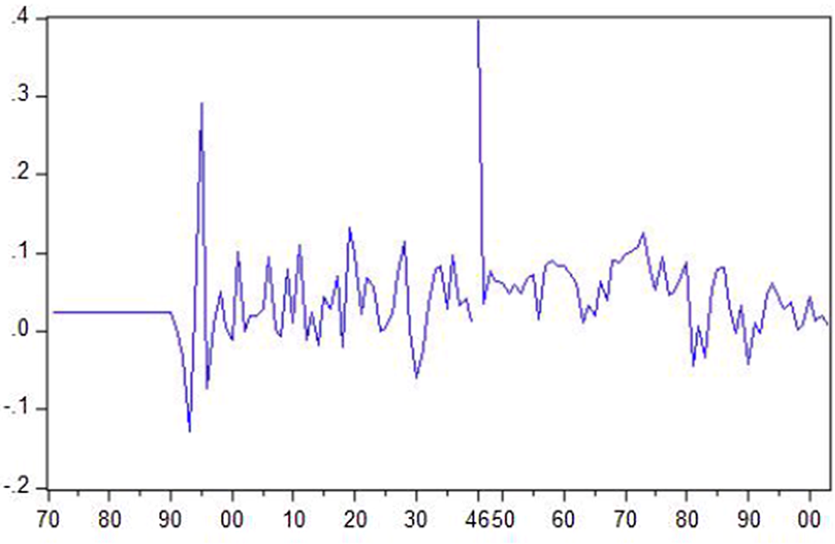
Figure 1. GDP growth.
The existing measures of both formal and informal political indicators for Brazil are yearly from 1919 to 2003 with the exclusion of the World War II period (1940–1945). In order to track political instability back to the year of 1870, we constructed our own informal and formal political instability series from 1870 to 1919 (see Figures A1 and A2 in the Online Appendix). In the spirit of Acemoglu et al. (Reference Acemoglu, Naidu, Restrepo and Robinson2019) and according to the definitions of the political instability variables (see below), we collect information on relevant political events from 1870 to 1930. Then, by comparing the data we constructed to the existing data from 1919 to 1930, we evaluate the accuracy of the new data series we generated. In the following subsections, we describe in detail the construction of the political instability indicators from 1870 to 1930 and how those political institutions series we generated match the existing data sets.
The substantial number of our political indicators we analyse below may introduce biases and inflate the measurement error by increasing the noise-to-signal ratio. To circumvent these concerns, we conduct principal component analysis (PCA) as well factor analysis (FA), in order to classify variables into components factors and hence check whether this kind of latent analysis confirms the dominant blocks of informal and formal political instability introduced by Campos and Karanasos (Reference Campos and Karanasos2008).Footnote 3 From this analysis, two main components/factors were extracted (with a zero-correlation coefficient). The first component has an eigenvalue of 2.53 and it consists of indicators that we ex ante classified as formal political instability, whereas the second component has an eigenvalue of 2.26 consisting of measurements that we defined as informal political instability. Moreover, based on the explained and unexplained variation of each of the two components the formal instability is more powerful than the informal one (the results of the PCA/FA analysis serve as a robustness check of our political instability taxonomy). Furthermore, among all informal indicators, guerrilla warfare and coups d’état display the lowest unexplained variation, whereas among the formal ones it is legislation selection and purges (figures not tabulated).
Jong-A-Pin (Reference Jong-A-Pin2009) argues that most studies that have focused on the effect of political instability on economic growth have constructed one dimensional index using either PCA, or discriminant analysis, or logit analysis. Nevertheless, there is strong evidence from political science that political instability is multidimensional, although there is no consensus as to the exact number of those dimensions. Thus, the results provided by the PCA may still suffer from measurement error, or, at least ignore some aspects of political instability when examining the effect on economic growth.
3.1 Changes in formal political institutions
Our formal political institution variables (in all tables these indicators are labelled as formal political instability) include eight dimensions, namely: changes in effective executive (the number of times in a year that effective control of the executive power changes hands, given that the new executive be independent of his predecessor), government crises (any rapidly developing situation that threatens to bring about the downfall of the present regime, excluding situations of revolt aimed at such an overthrow), legislative effectiveness,Footnote 4 legislative selections,Footnote 5 major constitutional changes (the number of basic alterations in the constitutional structure, we document that there were no major constitutional changes between the year 1891 and the Vargas Era), number of cabinet changes (the number of times in a year that a new premier is named and/or 50% of the cabinet posts are occupied by new ministers), purges, and size of cabinet.
With the exception of the government crisis and the purges, all other formal political events are recorded since the year 1870. There were no major changes for legislative effectiveness, legislative selections and number of cabinet changes during the First World War Period. According to the definition, the changes in effective executive are equal to the changes of the presidents.
Given the definition of the purges – any systematic elimination by jailing or execution of political opposition within the ranks of the regime or the opposition – we find that the last decades of the Second Empire were marked by considerable political instability. In the year 1884, records show that, out of a peacetime army of 13,500 men, more than 7,500 had been jailed for insubordination (Lima, Reference Lima1986). Based on Woodard (Reference Woodard2009) and Love (Reference Love1980), in 1891 and 1892, along with the rebellions and the change of the president, various purges took place. As existing data recorded another purge activity in the year 1930, we found the corresponding political history event in Bethell (Reference Bethell2008). In particular, soon after the 1930 revolution, a quick change among the armed forces had been adopted. The senior ranks were eliminated by a purge. By the end of 1930, nine of eleven major generals and 11 of –24 brigadier generals retired.
Although there is a clear definition of the government crisis, it is still hard to define which events or situations are rapidly developing that threaten to bring about the downfall of the present regime. The Paraguay War centralised government power, thus, there was almost no revolutionary revolt against the government for years to come. However, as Colson (Reference Colson1981) stated, the crisis of 1889 has long been seen as a turning point in Brazilian history. First of all, the Paraguay War raised massive public debts that seriously reduced the growth of the country. Then, the abolition of slavery gradually weakened the firm foundation of the monarchy – it had lost the support of vital groups such as the landowners (Hahner, Reference Hahner1969). More importantly, the war with Paraguay greatly increased the political power of the Brazilian army. Eventually, with the allowance of a discontented republican minority to grow more powerful (Republicanism), a group of army officers led by Manoel Deodoro da Fonseca launched a coup to proclaim the Republic on 15 November 1889. In light of this, we mark the first government crisis in Brazil during the time period between 1870 and 1930 as having occurred in the year 1889. Another government crisis which is recorded in existing data is for the year 1930. Similar to the crisis in 1889, the government crisis in 1930 resulted from multiple factors. Politically, the Tenente's revolt occurred in 1922 and then in 1924 had shaken the interior of Brazil without ever being defeated by the army. Then, the Old Republic suffered a big hit with the Great Depression that began in October 1929. Although limited at the beginning, the problem of overproduction became serious within 4–5 years. Brazilian exports fell about two-thirds within 7 years' time – from 1929 to 1935. Losing profit from coffee exports, the Sao Paulo oligarchy tried to stay in power disregarding the agreed alternation with Minas Gerais. This led to the end of the ‘politics of coffee with milk’. Those political crises together with the economic crisis led to the end of the Old Republic on 24 October 1930.
To sum up, in order to generate our own political instability series, we track all the political events yearly from 1870 to 1930. Next, we classified each event to its own category according to the definition which has been mentioned above. Finally, by comparing the data we generate to the existing ones from 1919 to 1930, we conclude that the series we generated from these events are basically correct.
3.2 Informal political instability
Our informal political instability variables include seven indicators. First of all, we identify the events that related to the anti-government demonstrations. As anti-government demonstrations are defined as peaceful government gatherings of at least 100 people, we find only one related political event which occurred in the year of 1904. With the approval of the law of Mandatory Vaccination, an uprising against the government's decisions broke out. The event began on the 10th of November, with a group of student demonstrations (Fausto, Reference Fausto1986). Although the movement quickly turned into a riot in the end, it was a peaceful demonstration in the first few days. In the following 26 years, until the year 1930, we cannot find any other information about anti-government demonstrations either from the political history resources.
Our second informal political instability measure, namely assassinations, is defined as any politically motivated murder or attempted murder of a high government official or politician. The only related event we found during the period of 1870–1919 is that Jose Gomes Pinheiro Machado, who was a Brazilian republican politician, was murdered in the year 1915 (Fausto, Reference Fausto1986). We also find two other assassinations in the year 1930. Earlier in February, Vice President Mello Vianna was shot at Monte Claros in the state of Minas Gerais and, in July, Joao Pessoa Cavalcanti de Albuquerque, who was the governor of Paraiba, was murdered (Fausto, Reference Fausto1986).
In the case of general strikes, there are none on the records before the year 1888 perhaps because Brazil was still under slavery. According to the definition of general strikes, a general strike involved at least 1,000 workers and aimed at government policies, we found that the first major strike in Brazil occurred in Rio de Janeiro in 1903 when workers at the Aliaca Textile Mill walked off. This strike paralysed Rio de Janeiro for 20 days when over 40,000 workers from all the city's textile mills demanded better conditions and pay (Hall and Spalding, Reference Hall and Spalding1986). The next short and unsuccessful strike was a general strike in the textile industry of Sao Paulo in 1907. Six years later, another large strike led by city's Federacao Operaria Syndical occurred in Rio Grande do Sul. In the year 1917, one of the largest general strikes broke out in Sao Paulo in July. According to Hall and Spalding (Reference Hall and Spalding1986), records show that about 50,000 people joined the movement. From the year 1919 to 1930, our existing data set shows that one strike happened in the year 1920 which is recorded by Everett (2011).
It is, sometimes, hard to distinguish guerrilla warfare from revolutions. In this paper, we define guerrilla warfare as armed activity, sabotage, or bombings carried on by independent bands of citizens or irregular forces and aimed at the overthrow of the present regime. According to this definition we found the Contestado War (Guerra do Contestado) that started in 1912 (Vinhas de Queiroz, Reference Vinhas de Queiroz1966). Clashes between settlers and landowners lasted for 4 years. During that time, with the support by the Brazilian states' police and military forces, around 9,000 houses were burned, and 20,000 people were killed. In the end, the guerrilla war was finally ended with the capture of the last leaders of the Contestado in August 1916. In examining the historical records, we also find two more guerrilla wars. The first one is the revolution of 1923 whereas the second one is the movements led by Luis Carlos Prestes in the year 1924 (Fausto, Reference Fausto1986).
The fifth measure of our informal political instability variable is the number of coups, which is defined as the number of extra constitutional or forced changes in the top government elites. Examining the historical record, it is clear that over the period of 1870–1930 only two bloodless coups occurred, in the year 1889 and 1930, respectively. As Roett (Reference Roett1999) stated, the traditional resources of support for the monarchy were seriously weakened at the end of the Second Empire. Firstly, on 15 November 1899 the Emperor was dethroned and Brazil passed from a centralised Empire to a federal republic by a bloodless coup (Fausto, Reference Fausto1986). Secondly, in the year 1930, after Vargas took power, he issued a decree which granted virtually dictatorial powers to the government and dissolved the congress. The latter has been characterised as a coup by Bethell (Reference Bethell2008).
Our sixth informal political indicator is revolutions defined as an illegal or forced change (or attempt) in the top governmental elite. During the 6 years from 1864 to 1870, Brazil, Argentina and Uruguay fought a bloody war with Paraguay. Due to the competition between the second President Deodoro da Fonseca and Vice President, Floriano Peixoto, soon after the formation of the First Republic, the first Revolt of the Navy (Revolta da Armada) broke out in 1891. The President dissolved the congress, provoking rebellions in Rio de Janeiro and in the southernmost state of Rio Grande do Sul (Hahner, Reference Hahner1969). One year later, a document sent by 13 generals to the president of the Republic called for new elections. President Floriano, who took office after the first revolt of the navy, suppressed the movement, and ordered the arrest of its leaders. In September of 1893, the second Revolt of the Navy (Revolta da Armada) broke out at Rio de Janeiro (Hahner, Reference Hahner1969). Although the naval insurgents still threatened the capital, the Federalists rapidly approached the southern borders of Sao Paulo. The Federalist Revolution, which lasted 2 years from 1893 to 1895, was defeated in the Battle of Passo Fundo. Moreover, in the same year of 1893, a bloodier conflict began. The Canudos War had a brutal end in October 1897, almost all the insurgents were killed by a large Brazilian army force (MacLachlan, Reference MacLachlan2003). A few years later, The Revolt of the Lash (Revolta da Chibata) broke in November 1910. There were about 2,400 sailors involved in this revolt. The rebellion had been planned for about 2 years and was triggered by severe punishment applied to the sailor Marcelino Rodriguez Menezes. The movement threatened to bomb the capital city of Rio de Janeiro (Schneider, Reference Schneider2009).
The last measure of our informal political instability variable is riots, which are defined as the violent demonstration or clash of more than 100 citizens. The riots before the First Republic have been documented in several books (Bethell, Reference Bethell1989, Macedo, Reference Macedo1998, Carneiro, Reference Carneiro1960). From 1873 to 1874 in southern Brazil, a clash which is called Revolt of the Muckers (Revolta dos Muckers) between two groups in one German community arose. From the end of 1874 to the middle of 1875, in the northeast of Brazil, a revolt called Quebra-Quilos (Revolta do Quebra-Quilos) against a new system of weights and measures broke out. In the year 1875, about 300 women went through the streets (armed with stones and sticks) in order to protest against the compulsory military draft on 30th August (Guerra das Mulheres). During the last decade of the Empire, the revolt of the penny (Revolta do Vintem) took place between 1879 and 1880 in Rio de Janeiro (Carneiro, Reference Carneiro1960). Another important revolt occurred in the city of Curitiba in 1883. Ten years after the first civilian president of the republic assumed power in 1904, an uprising against a government decision broke out (Fausto, Reference Fausto1986): it started as a demonstration, however, the movement turned into a riot in the end. Furthermore in 1914, the president's attempt to intervene in the northeast region neutralised the political power of the oligarchy in the state of Ceara. However, the attempt to replace the state governor triggered the clash called the Sedicao de Juazeiro. From 1919 until 1930, the existing data set shows three riots. The first one occurred in the year 1920 (Fausto (Reference Fausto1986) recorded a revolt without much details) whereas another two riots took place in the year 1930, namely Revolta da Princesa (Fausto Reference Fausto1986) and those following the assassination of Joao Pessoa.
3.3 Comparison with other measures of institutional development
How do our measures described above compare to the existing measures of Brazil's institutional development? In this sub-section, we will focus on comparisons with other common measures of institutional development. Although our definitions and coding differ from measurements of democracy and institutional development introduced in the previous literature, due to the fact that they are more granular, we can find some substantial correlations between our indicators and those introduced by Acemoglu et al. (Reference Acemoglu, Johnson and Robinson2002), Boix et al. (Reference Boix, Miller and Rosato2013), Lindberg et al. (Reference Lindberg, Coppedge, Gerring and Teorell2014) and Spruk (Reference Spruk2016a, Reference Spruk2016b). Acemoglu et al. (Reference Acemoglu, Johnson and Robinson2002) quantify institutions using among others the constraints on the executive (a variable described in Gurr (Reference Gurr1996), and later updated in Marshall et al. (Reference Marshall, Gurr and Jaggers2015)) from Polity III data set, which serves as a proxy for the level of concentration of political power in the hands of ruling groups. We explore how our coding matches that of Marshall et al. (Reference Marshall, Gurr and Jaggers2015). Despite the different scaling between our measures and that of Marshall et al. (Reference Marshall, Gurr and Jaggers2015) we notice from Figures A2.c, A2.d and A3.a (in the Online Appendix) that legislative effectiveness, legislative selection and executive constraints are highly correlated.
Boix et al. (Reference Boix, Miller and Rosato2013) update and describe an extensively used data set on democracy covering a very long period of time, from 1800 to 2007 and 219 countries and representing the most comprehensive dichotomous measure of democracy (see Figure A3.b). Figures A1.a, A2.h and A3.b show that there is a significant correlation between the dichotomous measure of democracy (Boix et al., Reference Boix, Miller and Rosato2013) and our indicators of demonstrations and size of the cabinet (informal and formal indicator, respectively). Looking at those three graphs we notice that up to 1945, when Brazil was democratically repressed, the number of demonstrations were almost zero and the size of the cabinet was small. This trend started reversing from 1950 and especially from 1980 onwards when democracy become more entrenched.
Lindberg et al. (Reference Lindberg, Coppedge, Gerring and Teorell2014) generated a data set that measures democracy, the so-called Varieties of Democracy Project (V-Dem). Due to the lack of consensus on how to measure democracy they emphasise its multidimensionality. Out of the five principles that they follow in order to conceptualise democracy, we estimate high-correlation coefficients between various: (1) electoral factors such as vote buying in elections, free and fair elections, head of state legislation in practice and party ban (see Figure A3.c), (2) liberal components such as executive constitution and freedom from political killings (see Figure A3.d), and some of our dimensions such as demonstrations, assassinations, riots and guerrilla warfare as well as legislative selection and size of cabinet (due to space limitations, we project only a sample of the electoral and liberal components).
Finally, Spruk (Reference Spruk2016a, Reference Spruk2016b) measured institutional changes and investigated the impact of ‘de jure’ and ‘de facto’ political institutions on the long-run economic growth for a large panel of countries in the period 1810–2000 (due to space limitations see Figure A3.e for a sample of those components). Compared with their data set we estimate high correlation between their de jure (and in particular competitiveness and openness of executive recruitment) and de facto components (civil liberties and political rights) and our informal (namely assassinations, demonstrations and guerrilla warfare) and formal (such as legislative effectiveness and legislative selection) institution indicators. The data for the de facto components, namely civil and political rights, were available from 1972 onwards for Brazil.
4. Econometric framework
The PARCH model was introduced by Ding et al. (Reference Ding, Granger and Engle1993)Footnote 6 and quickly gained currency in the economics and finance literature.Footnote 7 Let growth (y t) follow a white noise process augmented by the lagged value of the institutional variable and the in-mean effect of output volatility (h t) on output:


where x it is either the formal political institution or the informal political instability indicator.
In addition, {e t} are independently and identically distributed (i.i.d.) random variables with $E\lpar {e_t} \rpar = E\lpar {e_t^2 -1} \rpar = 0$ , where h t is the conditional variance of output growth, which is positive with probability one and is a measurable function of the sigma-algebra $\sum _{t-1}$
 , which is generated by {y t−1, y t−2, …}.
In other words, h t denotes the conditional variance of growth. In particular, h t is specified as an asymmetric PARCH(1,1) process with lagged growth included in the variance equation:

with

where δ (with δ ∈ (0,∞)) is the heteroscedasticity parameter, α and β are the ARCH and GARCH coefficients, respectively, ς with |ς|<1 is the leverage term and γ is the level term for the n-th lag of growth. The model imposes a Box–Cox power transformation of the conditional standard deviation process and the asymmetric absolute residuals, see equation (3) (following Ding et al. (Reference Ding, Granger and Engle1993) asymmetric effects were initially considered in our model, though they are insignificant and have hence been omitted). In order to distinguish the general PARCH model from a version in which δ is fixed (but not necessarily equal to 2) we refer to the latter as (P)ARCH.
The PARCH model increases the flexibility of the conditional variance specification by allowing the data to determine the power of growth for which the predicted structure in the volatility pattern is the strongest. This feature in the volatility process has important implications for the relationship between institutions, growth and its volatility. There is no strong reason for assuming that the conditional variance is a linear function of lagged squared errors. The common use of a squared term in this role is most likely to be a reflection of the normality assumption traditionally invoked. However, if we accept that growth data are very likely to have a non-normal error distribution, then the superiority of a squared term is unwarranted and other power transformations may be more appropriate.
The PARCH model could be considered as a standard GARCH model for observations that have been altered by a sign-preserving power transformation implied by a modified PARCH parameterisation. He and Teräsvirta (Reference He, Teräsvirta, Engle and White1999) argue that if the standard Bollerslev type of model is augmented by the heteroscedasticity parameter, the estimates of the ARCH and GARCH coefficients are almost certainly different. Furthermore, by squaring the growth rates one essentially imposes a structure on the data that might lead to sub-optimal modelling and forecasting performance relative to other power terms. To assess the severity of this assumption we investigate the sample autocorrelations of the power transformed absolute growth |y t|d for various positive values of d. Figure A4.a in the Online Appendix shows the auto-correlogram of |y t|d from lag 1 to lag 20 for d = 0.8, 1.0, 1.5, 2.0 and 2.5. The horizontal lines show the ±1.96/√T confidence interval (CI) for the estimated sample autocorrelation if the process y t is i.i.d. In our case T = 128, so CI = ±1.96/√T = ± 0.173. The sample autocorrelations for |y t|0.8 are greater than the sample autocorrelations of |y t|d for d = 1.0, 1.5, 2.0 and 2.5 at every lag up to at least 11 lags. Alternatively, this means that |y t|d has the strongest and slowest decaying autocorrelation when d = 0.8. In addition, note that at the vast majority of the lags |y t|d has the lowest autocorrelation when d is 2 and 2.5. To explore the choice of the PARCH process further, we calculate the sample autocorrelations of the absolute value of growth $\rho _\tau$ (δ) as a function of δ for lags τ = 1, 5, …, 30 and taking δ = 0.125, 0.25, …, 4.0. Figure A4.b shows the plot of the calculated $\rho _\tau$
 (δ). For example, for lag 1, there is a unique point δ* equal to 0.8 for the absolute growth, such that ρ 1(δ) reaches its maximum at this point: ρ 1(δ*) > ρ 1(δ) for δ ≠ δ*.
We also test whether the estimated power term is significantly different from 2 using Wald tests. The estimated power coefficient is significantly different from 2 (see Table A3, panel A). In addition, the best fitting specification is chosen according to the likelihood ratio results and the minimum value of the Akaike information criterion (AIC), see panel B of Table A3 for a sample of those results. Due to space limitations the remaining results are available upon request. These findings provide evidence against Bollerslev's specification and empirical justification of the PARCH process. In conclusion, the statistical significance of the in-mean effect greatly depends on the choice of the size of the heteroscedasticity parameter. If the power term surpasses a specific threshold, then the aforementioned effect might become insignificant. The latter suggests that if one assumes a linear link between a variable and its uncertainty a priori, then a significant association between the two might not be observed.
We present our main reasons in three interdependent blocs: the direct, indirect and dynamic (short- and long-run) effects. We proceed with the estimation of the PARCH(1,1) model in equations (1) and (2) in order to take into account the serial correlation observed in the levels and power transformations of our time series data. The tables in the Appendix report the estimated parameters of interest for the period 1870–2003. These were obtained by the quasi-maximum likelihood estimation, which is robust to the presence of normality as implemented in EVIEWS and described by Bollerslev and Wooldridge (Reference Bollerslev and Wooldridge1992).Footnote 8 Once heteroscedasticity has been accounted for, our specifications appear to capture the serial correlation in the power transformed growth series. Moreover, the tests for remaining serial correlation suggest that all the models for each individual institutional indicator seem to be well-specified since there is no remaining autocorrelation in either the standardised or squared standardised residuals at 5% statistical significance level (due to space limitations results are not tabulated but are available upon request).
Our set of variables tries to reflect the different explanations for the Brazilian performance previously put forward by economic historians. This set comprises seven measures of informal political instabilities and eight forms of formal political institutions. In order to study the direct effects of our set of explanatory variables, we specify model 1 with φ = 0 in equation (2), whereas model 2 with λ = 0 in equation (1) allows us to investigate their indirect impacts on growth.
5. Empirical results
In this section, our results are presented following the specific types of effects. We start with the estimation of the (P)ARCH(1,1) model in equations (1) and (2) in order to obtain our baseline results on direct (on mean economic growth) and indirect (via volatility) effects of political instability on growth (Tables 1a to 2b). Then we refine our main findings by estimating the dynamic (short- and long-run) as well as structural break impacts, respectively.
5.1 Direct impact on growth
Tables 1a and 1b report the results from our estimation of the PARCH(1,1) model for each one of the elements in our set of explanatory institutional variables. In this paper, we estimate models with lagged values of our explanatory variables as regressors. As we will see below the lagged direct effect on growth is equivalent to the short-run impact.
The parameter we are most interested in is λ (in the third column of the tables). The results reveal that the direct effects of informal political instabilities on economic growth are mostly negative and statistically significant (five out of seven), whereas the effects of formal political institution variables are negative and significant as well (six out of eight).
As for the in mean parameter (k), notice that in all cases the estimates are highly significant and positive, which is in line with the theoretical argument of Black (Reference Black1987). Also, the power term coefficients δ are rather stable, with the AIC choosing a PARCH specification with power terms in most of the cases equal to 1.00 (e.g. anti-government demonstrations, general strikes, changes in effective executive and the size of cabinet).
We find that our main explanatory factors, changes in formal political institutions and informal political instabilities, affect Brazil's economic growth negatively. Four measures of informal political instability (anti-government demonstrations, assassinations, general strikes and number of coups d’état) and three measures of formal political institutions (changes in effective executive, legislative effectiveness and number of cabinet changes) seem to play important roles in determining growth (see Section 5.3). Next we will investigate whether or not such powerful effects remain in the presence of indirect (via volatility) effects.
However, before proceeding we must note that one possible important drawback of the identification strategy is omitted variable bias. Even though we know from the work of Knack and Keefer (Reference Knack and Keefer1995) and Rodrik et al. (Reference Rodrik, Subramanian and Trebbi2004) onwards that the institutions trump the contribution of geography and trade in explaining cross-country income differences over time, it is impossible to isolate the confounding effects of human capital as a competing channel that feeds directly into growth rates. Glaeser et al. (Reference Glaeser, La Porta, Lopez-de-Silanes and Shleifer2004) show that poor countries tend to escape the poverty trap through human capital investment often pursued by benevolent dictators whereas Sachs, Diamond and others believe that geography plays a larger role. In addition, Gyimah-Brempong and De Camacho (Reference Gyimah-Brempong and De Camacho1998) argue that despite the growing literature on the link between political instability and economic growth in less developed countries and the realisation that human capital is a crucial part of long-term economic growth, none of these studies have investigated the impact of political instability on economic growth through human capital formation.
To address this issue, we control for the effect of human capital formation using the average years of education (data obtained from Spruk (Reference Spruk2016b)) and see whether controlling for human capital renders the effects of our key institutional explanatory variables weak, stronger or unchanged. Furthermore, to eliminate any direct confluence of political institutions induced by adverse physical geography (Miguel et al., Reference Miguel, Satyanath and Sergenti2004) we consider the variation in rainfall (rain) as well as in annual temperature (temp), which serve as observable measures of climatic shock (data obtained from the World Bank). Our findings show a positive (negative) impact of the average year of education (variation in temperature) on economic growth whereas the effect of both informal and formal political institutions (on output) remains negative with either the same or slightly weaker magnitude (see parameter estimates ξ and ζ in Tables A4.a and A4.b in the Online Appendix).
In addition, we detect a negative link between the variation of rain and growth although it is statistically insignificant (see parameter estimates θ in Tables A4.a and A4.b). Relatedly, a measure of culture would be beneficial to rule out the direct effects of culture on long-run growth. Although we are aware of the difficulty of tracking such a measure, we exploited the approach of McCleary and Barro (Reference McCleary and Barro2006) and utilise the fraction of the population that is Catholic and immigration rate as rough proxies for the effects of culture, which have been one of the defining characteristics of Brazil's economic and institutional history. The data available from the Brazilian Institute of Geography and Statistics (IBGE) were discontinued for both variables (e.g. the immigration rate is available only from 1870 to 1975). To address this lack of data and thus avoiding further decrease of observations in our sample, we include the immigration rate in our models separately. We find that there is a negative impact on output growth, though statistically insignificant (due to space limitations results are not reported but are available upon request).
Finally, to further assess the robustness of our baseline results we test whether or not the inclusion of financial development (measured by money supply, commercial bank deposits and deposits at bank of Brazil), trade openness and public deficit renders the impact of political instability on growth. Preliminary results show that both formal and informal political institutions still affect growth negatively (results are not reported due to space limitations).
5.2 Indirect impacts via growth volatility
One of the main advantages of the (P)ARCH framework is that it allows us to study not only the direct growth effects from the full set of explanatory variables described above, but also their indirect effects on economic growth through the predicted component of growth volatility (conditional on its past values).
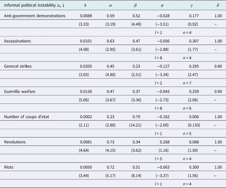
As we can see from Tables 1a and 1b, the effect of conditional or predicted volatility on growth is positive (k > 0) and statistically significant in all cases at conventional levels. Tables 2a and 2b report the estimation results for each one of the elements in our data set for what we call the indirect impact, which is the effect on growth via the volatility channel. The parameter we are most interested in is φ (in the fifth column of the aforementioned tables).
Our results show that the effects of both formal and informal political institutions are mostly negative and significant (with the exceptions of revolutions and major constitutional changes). We find that exogenous increases in political instability have a negative and significant indirect impact on growth. That is, less political instability is associated with a larger fraction of growth volatility, which is anticipated by the relevant economic agents. And the larger the share of the growth volatility that is anticipated, the higher the growth rates we observe (supporting the Black hypothesis). Therefore, political instability generates a negative-lagged direct effect on growth but also a substantial impact on the expected or conditional share of growth volatility and thus a negative indirect effect as well.
As far as the indirect effect is concerned, political uncertainty might reduce the return on future investments hence promoting incentives in delaying them which in turn contribute towards lower output growth. By observing a double negative effect (both direct and indirect) of political instability on output growth the consequences of the former on the latter are burdensome. Thus, macro as well as government policy theorists should (1) incorporate the analysis of political uncertainty into growth models and (2) try to avoid it.
To sum up, we find strong evidence that both formal and informal political institutions have a negative indirect (via volatility) impact on growth.
5.3 Joint estimation of direct and indirect effects
How robust are these baseline results? It seems that both formal and informal political institution variables are dominant influences. Specifically, we ask how the results for the political instability indicators change if we examine the indirect and direct effects jointly.
Tables 3a and 3b present the results when we include our political institution indicators in both the mean and variance equations. In particular, our parameter estimates show that informal political variables have the expected negative and statistically significant lagged direct impacts (see the λ column in Table 3a) with the exception of guerrilla warfare and riots. As far as the negative direct effect of formal political institutions on growth is concerned, they are significant in only three out of the eight cases. In other words, when we consider both direct and indirect effects, the negative direct impact of formal political institutions on growth falls slightly since it becomes insignificant for legislative selection and size of the cabinet.
5.4 Dynamic aspects
In this sub-section we investigate how short- and long-run considerations help us refine our baseline results. Another potential benefit from this exercise is that the required use of lags may help ameliorate any lingering concerns about endogeneity. In order to estimate short- and long-run relationships we employ the following error correction (P)ARCH form:

where θ and ζ capture the short- and long-run effects respectively, and φ is the speed of adjustment of the long-run relationship. This is accomplished by embedding a long-run growth regression into an autoregressive distributed lag model. In other words, the term in parenthesis contains the long-run growth regression, which acts as a forcing equilibrium condition:

where u t is I(0). The lag of the first difference of either the informal or formal political institution variable (Δx i,t−l) characterises the short-run effect. The condition for the existence of a long-run relationship (dynamic stability) requires that the coefficient on the error-correction term be negative and not lower than −2 (that is, −2 < φ < 0). We also take into account the PARCH effects by specifying the error term ɛ t, as follows:

where

Tables 4a and 4b report the results of estimations of short- and long-run parameters linking the explanatory variables with growth. In all cases, the estimated coefficients of the error correction term (φ) lie within the dynamically stable range (−2, 0). Generally speaking, from investigating whether dynamic considerations affect our conclusions, we find major differences in terms of short- and long-run effects. To be more specific, we find that, in total, 14 out of the 15 political institution variables have strong short-run effects whereas only five out of the 15 explanatory variables have long-run effects.
Next we discuss the results regarding the informal political factors and formal ones separately. We first focus our analysis on those obtained from the informal political instabilities. Table 4a presents the results. The estimated φ lies within the range −0.55 to −0.32, whereas θ and ζ capture the short- and long-run effects, respectively. With the exception of guerrilla warfare, all other estimates of the short-run coefficients (see the θ column) are significant and negative. However, the corresponding values for the long-run coefficients present a very different story, that is the negative short-run effects of anti-government demonstrations, general strikes and riots disappear in the long-run (see the ζ column in the table).
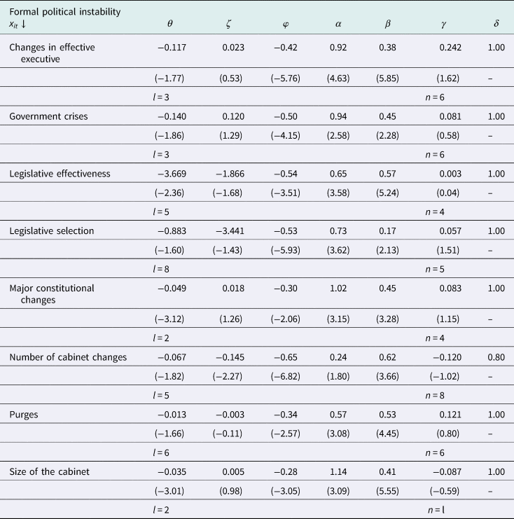
Similarly, we find strong evidence that formal political factors affect economic growth negatively (estimates of the short-run coefficients are significant and negative), whereas we observe long-run effects in only two out of the eight formal political indicators, namely legislative effectiveness and number of the cabinet changes (see Table 4b).
In summary, in the short-run, 14 political institution variables have a negative effect on Brazil's growth whereas in the long-run, only five political institutions (three informal and two formal ones) seem to affect growth negatively.
5.5 External validity
In this subsection, we will cross-validate our results with a country that has experienced similar magnitudes of political and institutional instability, namely Argentina. Campos and Karanasos (Reference Campos and Karanasos2008) investigated the growth volatility–political instability relationship using an econometric technique similar to ours for Argentina but using a smaller range of institutional variables and a slightly shorter time window which covers 1896–2000. They show that although informal political instability has a direct negative effect on growth, formal instability has an indirect impact, via the growth volatility. Our parameter estimates for Brazil indicate a strong direct and indirect effect of both informal and formal political instability indicators on growth.
Campos et al. (Reference Campos, Karanasos and Tan2012) extend the work of Campos and Karanasos (Reference Campos and Karanasos2008) by examining the impact of informal political instability on growth in the short- and long-run in Argentina. They find that the informal instability effects are substantially larger in the short- than in the long-run (Campos et al., Reference Campos, Karanasos and Tan2012). Similarly, we report that: (a) political instability has a negative effect on Brazil's growth in the short-run (whereas in the long-run only a few of the instability indicators affect growth negatively); and (b) both informal and formal political instability effects are, in most of the cases, larger in the short- than in the long-run. The latter provides evidence, in line with Campos and Nugent (Reference Campos and Nugent2002) and Murdoch and Sandler (Reference Murdoch and Sandler2004), for the notion that the duration of the political instability effect matters.
To facilitate our analysis further we plot (and compare) the level of Brazilian per capita GDP against the one of the Latin American (namely Argentina, Chile, Colombia, Uruguay and Venezuela) and Western European countries (i.e. France, Germany, Portugal, Spain and UK) for the period 1870–2003 (obtained from Bolt et al., Reference Bolt, Inklaar, de Jong and van Zanden2018). More specifically, Figures A5.a and A5.b in the Online Appendix report the level of Brazilian per capita GDP relative to Latin American and Western European countries, respectively. The graphs show that Brazil has the lowest GDP per capita compared to both groups of countries by a considerable amount for most of the sample period.
The region of Latin America consists of a number of countries that experienced various degrees of institutional change and political instability. The transition between the different political regimes was either smooth through stable constitutional changes or violent through revolutions, assassinations and military dictatorships. Figure A5.a suggests that despite the fact that most of Latin American countries displayed comparable degrees of political uncertainty the Brazilian economic welfare was only comparable to that of Colombia and Venezuela until around the 1910, although well behind after that period. On the contrary, Argentina that faced magnitudes of political unrest similar to that of Brazil enjoyed a much higher economic welfare.
5.6 Structural breaks
In order to investigate the potential role of structural breaks, we use the methodologies developed by Bai and Perron (Reference Bai and Perron2003) and Wald–Chow to observe whether or not there are any structural breaks in growth, informal as well as formal political institution indicators (see Table A5 in Online Appendix for a list of all the identified breaks). Under very general conditions on the data and the errors, Bai and Perron (Reference Bai and Perron2003) address the problem of testing for multiple structural changes. In addition to testing for the existence of breaks, these statistics identify the number and location of multiple breaks. In the case of the economic growth series, the Bai–Perron methodology supports three structural break points, which occur for the years 1893 (though statistically insignificant and hence omitted from the subsequent analysis), 1938 and 1979, respectively, whereas the Wald–Chow technique reports one break in 1893.
Based on the Bai–Perron test, for three measures of informal political instability (guerrilla warfare, number of coups d'etat and revolutions) and six measures of formal political institutions (namely changes in effective executive, government crises, legislative effectiveness, major constitutional changes, purges and size of the cabinet), we find no structural breaks. However, our Bai–Perron results support one structural break in anti-government demonstrations (dated 1964), assassinations (in 1978), and general strikes (in 1902). Additionally, we also find two structural breaks in riots during 1929 and 1964, respectively. We also detect one structural break for legislative selections and number of cabinet changes, which occur in 1939 and in 1889, respectively. As far as the Wald–Chow results are concerned, the breakpoints are substantially close to the ones provided by the Bai–Perron in most of the cases (see Online Appendix for further details and results from structural breaks modelling).
We find our results to be quite robust to the inclusion of the structural breaks. That is, both informal and formal political institutions have strong negative effects on growth and its volatility (see Tables A6.a to A7.b in the Online Appendix). As to the dynamic aspects, for three measures of informal political instability (namely assassinations, coups d'etat and revolutions) we find strong evidence of a negative impact on both short- and long-run, whereas three out of the four other measures (namely anti-government demonstrations, general strikes and riots) affect growth only in the short-run (Table A8.a). Similarly, with the exception of legislative effectiveness and number of cabinet changes, all other formal political institution variables have mostly a short-run negative effect on growth, see Table A8.b.
Interestingly, the causal direct, indirect and the short-run impacts from anti-government demonstrations and assassinations become weaker after the identified structural breaks in 1964 and 1978, respectively (see the λ d and φ d columns in Tables A6.a and A7.a, and the θ d column in Table A8.a). By the same token, (1) the direct effect of legislative selection is stronger before 1939 (see the λ d column in Table A6.b) and (2) the indirect and short-run impacts of cabinet changes are stronger before 1889 (see the φ d column in Table A7.b and the θ d column in Table A8.b).
To further corroborate our structural break analysis, we consider whether the break dates of major political events, which were tracked via the Bai–Perron test, are associated with the structural breaks in Brazil's long-run growth path. By utilising the Wald–Chow test (with known breakpoints, since the break dates are postulated by the political events we used to construct our measures of political institutions) we find that in all cases but one (demonstrations in 1964) the political events triggered highly significant structural breaks on growth as well. For instance, for assassinations we detect a structural break in 1978, which in turn seem to have triggered a statistically significant structural break in the Brazilian GDP as well (see panel B of Table A9 in the Online Appendix). In addition, we notice that the estimated breakpoints of political events are very close to the structural breakpoints of growth provided in panel A. This analysis indicates that our parametric estimates (from equations (A.1) to (A.4)) pick up indeed the effect of instability on growth and not some other unelaborated channels of influence.
Finally, our structural break analysis suggests that the landmark dates of institutional change in Brazil's economic and institutional history (namely the end of the Second Empire in 1889, the economic collapse of 1929 and the subsequent revolution of 1930 as well as the enforcement of a military government for almost 20 years until 1985) are highly associated with the structural breaks of growth and/or our political instability indicators.
5.7 Discussion
In this sub-section, we discuss and summarise our results. Our parameter estimates show that informal and formal political institutional indicators affect Brazil's economic growth negatively, both directly and indirectly via the growth volatility channel. To investigate the robustness of our baseline results we consider whether or not these results change if we allow for the indirect and direct effects jointly. With respect to our informal indicators, direct and indirect effects remain negatively strong, whereas for our formal measurements the negative direct impact on growth falls slightly. Finally, we estimate the short- and long-run effect of political institutions on growth. In short, the results suggest a strong negative link between instability and growth in the short-run and a weak one in the long-run.
To further strengthen our results, we consider the issue of omitted variable bias. To address this drawback of our identification strategy we control for the effect of human capital formation as well as the immigration rate. Moreover, to rule out any direct confluence of political instability induced by adverse physical geography we also use the variation in rainfall and annual temperature. After controlling for the aforementioned factors, our estimations concerning the impact of formal and informal political instability on growth remain largely unchanged.
Our results are consistent with those of other countries in Latin America that experienced similar magnitudes of political and institutional arrest such as Argentina. Similar to our paper that argues in favour of a negative relationship between political instability and growth for the Brazilian case, Campos and Karanasos (Reference Campos and Karanasos2008) and Campos et al. (Reference Campos, Karanasos and Tan2012) find a negative link between political instability and Argentinian economic growth for a similar time window, though a slightly shorter one. Our results are also consistent with the findings of other studies on the effect of political instability on growth. For instance, De Gregorio (Reference De Gregorio1992) and Gyimah-Brempong and De Camacho (Reference Gyimah-Brempong and De Camacho1998) find a direct negative effect of political instability on growth in a sample of 12 and 18 Latin American countries, respectively.
Considering the role of structural breaks, we find that our findings are robust to the inclusion of structural break dummies. In particular by employing the Bai–Perron and Wald–Chow statistics we find among others: (a) three breaks in the economic growth series for the years 1893, 1938 and 1979, (b) the landmark dates of institutional change in Brazil's economic and institutional history are closely associated with the structural breaks of growth as well as our political instability indicators, (c) informal and formal institutions have strong negative effects on growth and its volatility, (d) there is a strong impact of instability on growth in the short-run, and (e) under the Wald–Chow technique our parametric estimates pick up the effect of instability on growth and not some other unelaborated channels of influence.
There are not, after extensive search and to the best of our knowledge, theoretical models that differentiate growth effects by type of political instability. What there is instead is the recognition that political instability can escalate and with it, the relative magnitude of its growth effects can increase (Campos and Gassebner, Reference Campos and Gassebner2013). For instance, general strikes can escalate into mass demonstrations, which can escalate into riots, which by their turn can escalate into guerrilla conflicts. The growth effects differ along the characteristics of each of these modalities. For example, a guerrilla conflict can have larger negative effects on growth if more widespread and longer lasting than, say, mass demonstrations. Yet, if guerrillas are constrained to smaller and less populated areas, their effects should be relatively smaller.
6. Conclusions and future research
Using a new and unique data for Brazil from 1870 to 2003 as well as a PARCH framework we attempted to provide answers to the following questions: What is the relationship between political instability, institutional change, economic growth and (predicted) growth volatility? Are these effects fundamentally and systematically different? Does the intensity and the direction of these effects vary over time, in general and in particular, do they vary with respect to short- versus long-run considerations?
Our empirical results show that the majority of the formal political institutions and informal political instability indicators have strong negative direct and indirect effects on economic growth in Brazil. From investigating whether dynamic considerations affect our conclusions, we find important differences in terms of the short- and long-run behaviour of our key variables. Specifically, although strong negative impacts are found in the short-run (14 out of 15), the effects for the long-run are weaker (five out of 15). For two informal political instabilities (assassinations and number of coups) and two formal political institutions ones (legislative effectiveness and number of cabinet changes), all four effects (direct/indirect, short- and long-run) are highly significant.
The main goal of this study was to assess the role of the institutions on Brazilian economic growth by specifically disentangling the changes in formal political institutions and informal political instability components. There are some limitations of the present study that should be addressed in future work. One such limitation is that the empirical evidence does not provide a definite account of the causal link between institutions and growth since we do not exploit plausibly exogenous sources of variation in Brazil's long-run growth and do not use a research design that would allow us to exploit such channels. However, we have addressed the omitted variable bias issue in great detail. Nevertheless, these concerns are greatly alleviated (with careful identification strategies and the lagged estimations or structural breaks) to the extent that our regressions yield consistent results. In addition, due to the historical scope of this paper, certain factors, such as culture, which potentially directly affect economic growth could not be considered due to the unavailability of data. Future studies should also investigate the link between political institutions and economic growth in a panel of developing countries as well as the relationship between institutional change and political instability. Finally, a simulation analysis of how growth rate would have been in the absence of some institutional shocks would clearly represent progress and is something we recommend future research should try to address.
Appendix
See Tables 1a to 4a and 1b to 4b.
Table 1a. Direct effect of informal political instability on GDP growth
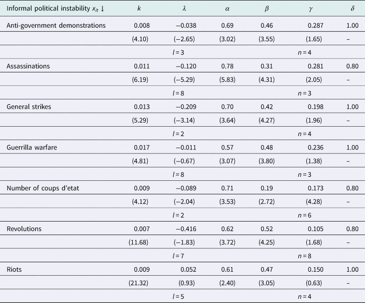
Table 1b. Direct effect of formal political instability on GDP growth
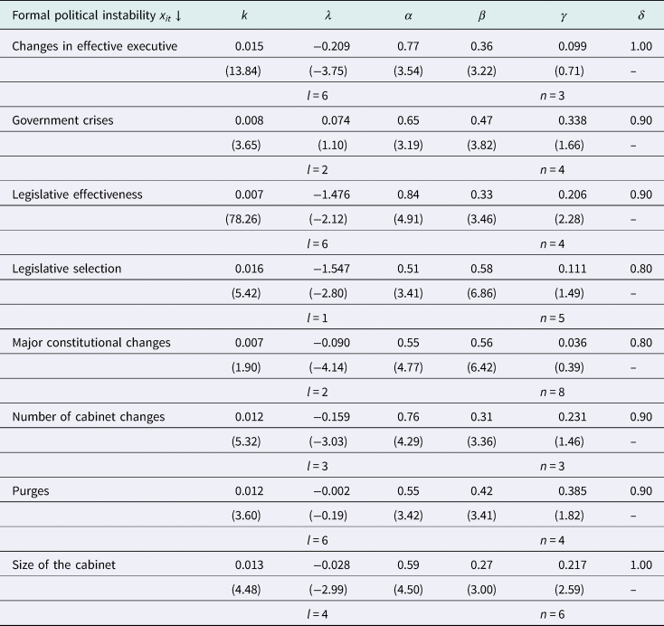
Table 2a. Indirect effect of informal political instability on GDP growth

Table 2b. Indirect effect of formal political instability on GDP growth

Table 3a. Direct and indirect effects of informal political instability on GDP growth

Table 3b. Direct and indirect effects of formal political instability on GDP growth

Table 4a. The short- and long-run effects of informal political instability on GDP growth

Table 4b. The short- and long-run effects of formal political instability on GDP growth