1 Introduction
A successful method for modelling thermoacoustic instabilities is the truncated harmonic balance method (Dowling Reference Dowling1997; Noiray et al.
Reference Noiray, Durox, Schuller and Candel2008; Boudy et al.
Reference Boudy, Durox, Schuller, Jomaas and Candel2011; Palies et al.
Reference Palies, Durox, Schuller and Candel2011). This approach has so far been restricted to situations with only one mode of the system, close to the Hopf bifurcation, and to longitudinal configurations. Under these restrictions, the method involves the study of the solutions of a nonlinear dispersion relation
 $f(\unicode[STIX]{x1D714},A)=0$
that depends on the amplitude
$f(\unicode[STIX]{x1D714},A)=0$
that depends on the amplitude
 $A>0$
of the oscillation. See the end of the paper for a Nomenclature. A limit cycle is formed if there exists a non-trivial solution with a zero growth rate, i.e.
$A>0$
of the oscillation. See the end of the paper for a Nomenclature. A limit cycle is formed if there exists a non-trivial solution with a zero growth rate, i.e.
 $A>0,\unicode[STIX]{x1D714}\in \mathbb{R}$
. In the analysis, there is no need to study the phase
$A>0,\unicode[STIX]{x1D714}\in \mathbb{R}$
. In the analysis, there is no need to study the phase
 $\unicode[STIX]{x1D711}$
of the oscillation, because the system consists of only one self-excited oscillator and is then invariant under a shift of the time variable. For a detailed description, we refer the reader to Dowling (Reference Dowling1997), Noiray et al. (Reference Noiray, Durox, Schuller and Candel2008).
$\unicode[STIX]{x1D711}$
of the oscillation, because the system consists of only one self-excited oscillator and is then invariant under a shift of the time variable. For a detailed description, we refer the reader to Dowling (Reference Dowling1997), Noiray et al. (Reference Noiray, Durox, Schuller and Candel2008).
The application of this framework to annular combustors is more challenging because of the presence of azimuthal modes. These appear as mode pairs, with amplitudes
 $A_{1}$
and
$A_{1}$
and
 $A_{2}$
(say), because of the discrete rotational symmetry of the problem. Although the system remains time invariant to a temporal shift, the phase difference of the oscillations of the two modes, defined as
$A_{2}$
(say), because of the discrete rotational symmetry of the problem. Although the system remains time invariant to a temporal shift, the phase difference of the oscillations of the two modes, defined as
 $\unicode[STIX]{x1D711}\equiv \unicode[STIX]{x1D711}_{1}-\unicode[STIX]{x1D711}_{2}$
, plays a role in the dynamics. This leads to finding the solutions of a nonlinear dispersion relation
$\unicode[STIX]{x1D711}\equiv \unicode[STIX]{x1D711}_{1}-\unicode[STIX]{x1D711}_{2}$
, plays a role in the dynamics. This leads to finding the solutions of a nonlinear dispersion relation
 $f(\unicode[STIX]{x1D714},A_{1},A_{2},\unicode[STIX]{x1D711})=0$
and evaluating their stability. Some introductory work has been carried out by Campa, Cinquepalmi & Camporeale (Reference Campa, Cinquepalmi and Camporeale2013), Campa & Camporeale (Reference Campa and Camporeale2014) using a Helmholtz solver, where the stability with respect to only the amplitude of the mode was considered.
$f(\unicode[STIX]{x1D714},A_{1},A_{2},\unicode[STIX]{x1D711})=0$
and evaluating their stability. Some introductory work has been carried out by Campa, Cinquepalmi & Camporeale (Reference Campa, Cinquepalmi and Camporeale2013), Campa & Camporeale (Reference Campa and Camporeale2014) using a Helmholtz solver, where the stability with respect to only the amplitude of the mode was considered.
Low-order state-space models overcome this difficulty (Schuermans, Paschereit & Monkewitz Reference Schuermans, Paschereit and Monkewitz2006; Noiray, Bothien & Schuermans Reference Noiray, Bothien and Schuermans2011; Ghirardo & Juniper Reference Ghirardo and Juniper2013; Noiray & Schuermans Reference Noiray and Schuermans2013). They allow for the discussion of not just the amplitude of the solutions, but also the temporal evolution of the system and the stability of the solutions, features missing in the truncated harmonic balance method. Usually the method of averaging is applied to the state-space model, allowing a discussion of the temporal evolution of the two amplitudes
 $A_{1},A_{2}$
and of the phase difference
$A_{1},A_{2}$
and of the phase difference
 $\unicode[STIX]{x1D711}$
. The proposed fluctuating heat release rate model is limited in those studies to simple phenomenological expressions, in terms of the acoustic pressure and/or the acoustic azimuthal velocity. Also, only systems with fluctuating heat release rate uniformly distributed along the circumference were studied.
$\unicode[STIX]{x1D711}$
. The proposed fluctuating heat release rate model is limited in those studies to simple phenomenological expressions, in terms of the acoustic pressure and/or the acoustic azimuthal velocity. Also, only systems with fluctuating heat release rate uniformly distributed along the circumference were studied.
This paper bridges the gap between low-order state-space models and the truncated harmonic balance approach. We first show in § 2 that the equations of the low-order model can be obtained by studying the governing equations of the problem as weakly nonlinear. We then show how to exploit the describing function in applying the method of temporal averaging in § 3. This allows the flame response to remain generic, in contrast with all previous studies that considered a specific fluctuating heat release rate model. This allows us to prove with generality many properties of thermoacoustic oscillations in rotationally symmetric annular chambers. In particular we discuss the conditions under which spinning and standing waves are stable attractors of the system, and provide measurable quantities in experiments, which allow the validity of the hypotheses of this model to be tested.
We then present in § 4 an example that illustrates this theory. The example is the first analytical study of an annular combustor capable of exhibiting thermoacoustic triggering, and shows that flames responding with a weak gain at small amplitudes and with a strong gain at large amplitudes can lead to self-excited stable standing and spinning solutions in annular configurations. Finally we validate in § 5 this theory for the experiment of Bourgouin et al. (Reference Bourgouin, Durox, Moeck, Schuller and Candel2015) and draw the conclusions in § 6.
2 Governing equations
We discuss the geometry of the problem in § 2.1 and the modelling of the fluctuating heat release rate in § 2.2. We introduce the governing equations in § 2.3, both in the time domain and the frequency domain. We discuss the degeneracy of the linear solutions in the frequency domain in § 2.4. In § 2.5 we carry out the weakly nonlinear analysis of the problem, which consists of two steps. Firstly, we increase/reduce the flame response until the linear solution is neutrally stable, and calculate its spatial structure. Then, we project the original nonlinear governing equations on this structure, which is assumed to change very little in the nonlinear regime because the system is weakly nonlinear.
The resulting truncated equations describe the temporal evolution of the amplitudes of two standing modes describing the whole acoustic field. These two amplitudes are two damped oscillator, coupled nonlinearly through the fluctuating heat release rate. The two oscillators’ equations were already derived by Schuermans et al. (Reference Schuermans, Paschereit and Monkewitz2006), Noiray et al. (Reference Noiray, Bothien and Schuermans2011) and Ghirardo & Juniper (Reference Ghirardo and Juniper2013) for a fluctuating heat release rate uniformly distributed in the azimuthal direction using a Galerkin base instead.
2.1 Problem geometry
We adopt cylindrical coordinates
 $z,r,\unicode[STIX]{x1D703}$
, with the
$z,r,\unicode[STIX]{x1D703}$
, with the
 $z$
-axis corresponding to the axis of the combustion chamber and
$z$
-axis corresponding to the axis of the combustion chamber and
 $\unicode[STIX]{x1D703}$
in
$\unicode[STIX]{x1D703}$
in
 $[0\,,\,2\unicode[STIX]{x03C0})$
. We assume that a number
$[0\,,\,2\unicode[STIX]{x03C0})$
. We assume that a number
 $N_{b}$
of equal burners are equispaced along the annulus and that each of the
$N_{b}$
of equal burners are equispaced along the annulus and that each of the
 $N_{b}$
sectors has the same geometry. The problem is then invariant to the group of
$N_{b}$
sectors has the same geometry. The problem is then invariant to the group of
 $N_{b}$
-fold rotational symmetry
$N_{b}$
-fold rotational symmetry
 $C_{N_{b}}$
, with the fundamental domain being a sector spanning the angle
$C_{N_{b}}$
, with the fundamental domain being a sector spanning the angle
 $\unicode[STIX]{x0394}\unicode[STIX]{x1D703}\equiv 2\unicode[STIX]{x03C0}/N_{b}$
.
$\unicode[STIX]{x0394}\unicode[STIX]{x1D703}\equiv 2\unicode[STIX]{x03C0}/N_{b}$
.
We assume that the flames are acoustically compact, so that the fluctuating heat release rate is concentrated at the locations of the burners:
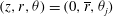
 $$\begin{eqnarray}q(\boldsymbol{x},t)=\mathop{\sum }_{j=1}^{N_{b}}q_{j}(t)\unicode[STIX]{x1D6FF}(\boldsymbol{x}-\boldsymbol{x}_{j}),\quad \boldsymbol{x}\equiv (z,r,\unicode[STIX]{x1D703}),\boldsymbol{x}_{j}\equiv (0,\overline{r},\unicode[STIX]{x1D703}_{j}),\end{eqnarray}$$
where
 $\unicode[STIX]{x1D6FF}$
is the Dirac delta in three dimensions,
$\unicode[STIX]{x1D6FF}$
is the Dirac delta in three dimensions,
 $\overline{r}$
is the radial position of the burners and the plane
$\overline{r}$
is the radial position of the burners and the plane
 $z=0$
is at the interface between the combustion chamber and the burners, which are located at the azimuthal positions
$z=0$
is at the interface between the combustion chamber and the burners, which are located at the azimuthal positions
 $\unicode[STIX]{x1D703}_{j}$
, equispaced by
$\unicode[STIX]{x1D703}_{j}$
, equispaced by
 $\unicode[STIX]{x0394}\unicode[STIX]{x1D703}$
. We number the burners in anticlockwise direction, and we choose a frame of reference so that the first burner is positioned at
$\unicode[STIX]{x0394}\unicode[STIX]{x1D703}$
. We number the burners in anticlockwise direction, and we choose a frame of reference so that the first burner is positioned at
 $$\begin{eqnarray}\unicode[STIX]{x1D703}_{1}=\frac{\unicode[STIX]{x03C0}}{4}+\frac{\unicode[STIX]{x0394}\unicode[STIX]{x1D703}}{4}\unicode[STIX]{x1D701}\,\left\{\begin{array}{@{}ll@{}}\unicode[STIX]{x1D701}\in \{0,2\}\quad & \text{if }N_{b}\text{ is even}\\ \unicode[STIX]{x1D701}\in \{0,1,2,3\}\quad & \text{if }N_{b}\text{ is odd}.\end{array}\right.\end{eqnarray}$$
The addition of the coefficient
 $\unicode[STIX]{x1D701}$
is arbitrary and corresponds to a simple rotation of the frame of reference, which will be useful later. This is exemplified in figure 1 for an odd
$\unicode[STIX]{x1D701}$
is arbitrary and corresponds to a simple rotation of the frame of reference, which will be useful later. This is exemplified in figure 1 for an odd
 $N_{b}=5$
number of burners.
$N_{b}=5$
number of burners.

Figure 1. Example of the position of the frame of reference for different values of
 $\unicode[STIX]{x1D701}$
for a number
$\unicode[STIX]{x1D701}$
for a number
 $N_{b}=5$
of burners. The burners are represented with black discs, and the large circles are the internal and external walls of the combustion chamber. In general the position at the angle
$N_{b}=5$
of burners. The burners are represented with black discs, and the large circles are the internal and external walls of the combustion chamber. In general the position at the angle
 $\unicode[STIX]{x1D703}=\unicode[STIX]{x03C0}/4$
:
$\unicode[STIX]{x1D703}=\unicode[STIX]{x03C0}/4$
:
 $\bullet$
for
$\bullet$
for
 $\unicode[STIX]{x1D701}=0$
is occupied by a burner;
$\unicode[STIX]{x1D701}=0$
is occupied by a burner;
 $\bullet$
for
$\bullet$
for
 $\unicode[STIX]{x1D701}=2$
is equispaced between two adjacent burners;
$\unicode[STIX]{x1D701}=2$
is equispaced between two adjacent burners;
 $\bullet$
for
$\bullet$
for
 $\unicode[STIX]{x1D701}=1$
is
$\unicode[STIX]{x1D701}=1$
is
 $3\unicode[STIX]{x0394}\unicode[STIX]{x1D703}/4$
far from the preceding burner and
$3\unicode[STIX]{x0394}\unicode[STIX]{x1D703}/4$
far from the preceding burner and
 $\unicode[STIX]{x0394}\unicode[STIX]{x1D703}/4$
far from the next.
$\unicode[STIX]{x0394}\unicode[STIX]{x1D703}/4$
far from the next.
Some designs feature a mean velocity
 $U_{\unicode[STIX]{x1D703}}$
in the azimuthal direction along the combustion chamber annulus. A non-zero azimuthal mean flow
$U_{\unicode[STIX]{x1D703}}$
in the azimuthal direction along the combustion chamber annulus. A non-zero azimuthal mean flow
 $U_{\unicode[STIX]{x1D703}}$
has two effects. Firstly, a non-zero
$U_{\unicode[STIX]{x1D703}}$
has two effects. Firstly, a non-zero
 $U_{\unicode[STIX]{x1D703}}$
makes one of the two spinning modes rotate faster and the other slower, and makes standing modes slowly rotate with pressure and velocity nodes moving at the speed of the mean azimuthal flow. See for example Wolf et al. (Reference Wolf, Staffelbach, Balakrishnan, Roux and Poinsot2010) for numerical evidence and a discussion, and refer to Bauerheim et al. (Reference Bauerheim, Salas, Nicoud and Poinsot2014), Bauerheim, Cazalens & Poinsot (Reference Bauerheim, Cazalens and Poinsot2015) for a detailed analysis of this first effect of
$U_{\unicode[STIX]{x1D703}}$
makes one of the two spinning modes rotate faster and the other slower, and makes standing modes slowly rotate with pressure and velocity nodes moving at the speed of the mean azimuthal flow. See for example Wolf et al. (Reference Wolf, Staffelbach, Balakrishnan, Roux and Poinsot2010) for numerical evidence and a discussion, and refer to Bauerheim et al. (Reference Bauerheim, Salas, Nicoud and Poinsot2014), Bauerheim, Cazalens & Poinsot (Reference Bauerheim, Cazalens and Poinsot2015) for a detailed analysis of this first effect of
 $U_{\unicode[STIX]{x1D703}}$
in a linear framework. Secondly, a non-zero
$U_{\unicode[STIX]{x1D703}}$
in a linear framework. Secondly, a non-zero
 $U_{\unicode[STIX]{x1D703}}$
bends the flames in the azimuthal direction, orthogonally to the burner’s axis. This leads to a loss of axisymmetry of the mean flame shape, and this loss of axisymmetry is in turn a necessary condition for the flame to have a non-zero linear response to azimuthal velocity perturbations, as proven by Acharya & Lieuwen (Reference Acharya and Lieuwen2014). In most cases however
$U_{\unicode[STIX]{x1D703}}$
bends the flames in the azimuthal direction, orthogonally to the burner’s axis. This leads to a loss of axisymmetry of the mean flame shape, and this loss of axisymmetry is in turn a necessary condition for the flame to have a non-zero linear response to azimuthal velocity perturbations, as proven by Acharya & Lieuwen (Reference Acharya and Lieuwen2014). In most cases however
 $U_{\unicode[STIX]{x1D703}}$
is very small compared to the speed of sound, and is fixed to zero in the following. This introduces
$U_{\unicode[STIX]{x1D703}}$
is very small compared to the speed of sound, and is fixed to zero in the following. This introduces
 $N_{b}$
reflection planes that are parallel to the combustor axis and pass through the middle of one segment, so that the problem is invariant to the pyramidal group of symmetry
$N_{b}$
reflection planes that are parallel to the combustor axis and pass through the middle of one segment, so that the problem is invariant to the pyramidal group of symmetry
 $C_{N_{b}v}$
.
$C_{N_{b}v}$
.
2.2 Flame response
In this study, we assume that the flame response to the acoustic field is known, both in the linear and nonlinear regime. A common modelling approach consists of expressing the fluctuating heat release rate
 $q_{j}$
of the
$q_{j}$
of the
 $j$
th flame in terms of only the acoustic axial velocity
$j$
th flame in terms of only the acoustic axial velocity
 $v_{j}$
just upstream of the burner. Doing so, we assume that the azimuthal, acoustic velocity
$v_{j}$
just upstream of the burner. Doing so, we assume that the azimuthal, acoustic velocity
 $u$
does not affect the response. This last point is proved theoretically in the linear limit for axisymmetric premixed flames in Acharya et al. (Reference Acharya, Shreekrishna and Lieuwen2012). This influence is experimentally verified to be small at low amplitudes of transverse forcing for the cases of a burner positioned at pressure/velocity nodes and for the case where it is swept by a spinning wave, where both
$u$
does not affect the response. This last point is proved theoretically in the linear limit for axisymmetric premixed flames in Acharya et al. (Reference Acharya, Shreekrishna and Lieuwen2012). This influence is experimentally verified to be small at low amplitudes of transverse forcing for the cases of a burner positioned at pressure/velocity nodes and for the case where it is swept by a spinning wave, where both
 $u$
and
$u$
and
 $v$
are excited at the same time (Saurabh et al.
Reference Saurabh, Steinert, Moeck and Paschereit2014). This effect is usually not taken into account because little is known in the nonlinear regime, i.e. at amplitudes of oscillation typical of self-excited thermoacoustic oscillations. In this paper we make the same assumption, but point out that the nonlinear effect of the transverse azimuthal velocity
$v$
are excited at the same time (Saurabh et al.
Reference Saurabh, Steinert, Moeck and Paschereit2014). This effect is usually not taken into account because little is known in the nonlinear regime, i.e. at amplitudes of oscillation typical of self-excited thermoacoustic oscillations. In this paper we make the same assumption, but point out that the nonlinear effect of the transverse azimuthal velocity
 $u$
on each flame has been investigated by Ghirardo & Juniper (Reference Ghirardo and Juniper2013). It does not affect the linear stability properties of the system, but it does affect the nonlinear dynamics, and can explain stable standing solutions in axisymmetric annular chambers.
$u$
on each flame has been investigated by Ghirardo & Juniper (Reference Ghirardo and Juniper2013). It does not affect the linear stability properties of the system, but it does affect the nonlinear dynamics, and can explain stable standing solutions in axisymmetric annular chambers.
The longitudinal fluctuating velocity
 $v_{j}$
oscillating in the
$v_{j}$
oscillating in the
 $j$
th burner can be expressed as a linear time-invariant operator of the acoustic pressure difference
$j$
th burner can be expressed as a linear time-invariant operator of the acoustic pressure difference
 $\unicode[STIX]{x0394}p_{j}$
between the two sides of the burner, which are the chamber and the plenum. The burners are assumed to be acoustically compact (Blimbaum et al.
Reference Blimbaum, Zanchetta, Akin, Acharya, O’Connor, Noble and Lieuwen2012), which allows them to be modelled as lumped elements. However, if we consider one mode oscillating harmonically in time, and we assume that the burner transfer function of the lumped element does not depend on the amplitude of oscillation (as validated for example in Ćosić, Moeck & Paschereit (Reference Ćosić, Moeck and Paschereit2014)), then
$\unicode[STIX]{x0394}p_{j}$
between the two sides of the burner, which are the chamber and the plenum. The burners are assumed to be acoustically compact (Blimbaum et al.
Reference Blimbaum, Zanchetta, Akin, Acharya, O’Connor, Noble and Lieuwen2012), which allows them to be modelled as lumped elements. However, if we consider one mode oscillating harmonically in time, and we assume that the burner transfer function of the lumped element does not depend on the amplitude of oscillation (as validated for example in Ćosić, Moeck & Paschereit (Reference Ćosić, Moeck and Paschereit2014)), then
 $\unicode[STIX]{x0394}p_{j}$
is proportional to
$\unicode[STIX]{x0394}p_{j}$
is proportional to
 $p_{j}$
, and one can express
$p_{j}$
, and one can express
 $v_{j}$
as a linear operator of the local value of the pressure in the chamber
$v_{j}$
as a linear operator of the local value of the pressure in the chamber
 $p_{j}$
. The same reasoning applies also to two degenerate azimuthal modes oscillating at the same frequency, as will be the case in the following.
$p_{j}$
. The same reasoning applies also to two degenerate azimuthal modes oscillating at the same frequency, as will be the case in the following.
In particular, we model the fluctuating heat release rate as a time-invariant operator
 ${\mathcal{Q}}$
:
${\mathcal{Q}}$
:
 $$\begin{eqnarray}q_{j}(t)={\mathcal{Q}}[p_{j}(t)].\end{eqnarray}$$
The operator
 ${\mathcal{Q}}$
contains all the complexity of the relation between
${\mathcal{Q}}$
contains all the complexity of the relation between
 $p_{j}$
and
$p_{j}$
and
 $q_{j}$
, and is nonlinear. We restrict our study to operators
$q_{j}$
, and is nonlinear. We restrict our study to operators
 ${\mathcal{Q}}$
that, excited with a harmonic input
${\mathcal{Q}}$
that, excited with a harmonic input
 $p=A\cos (\unicode[STIX]{x1D714}t)$
, respond strongly at the same input frequency
$p=A\cos (\unicode[STIX]{x1D714}t)$
, respond strongly at the same input frequency
 $\unicode[STIX]{x1D714}$
and weakly at higher harmonics
$\unicode[STIX]{x1D714}$
and weakly at higher harmonics
 $2\unicode[STIX]{x1D714},3\unicode[STIX]{x1D714},\ldots$
. This is a feature of flames, acting like a low-pass filter on the acoustic input (Schuller, Durox & Candel Reference Schuller, Durox and Candel2003). This, together with the acoustics being a narrow-band filter, is one of the reasons why frequency-domain calculations truncated at the first harmonic have proven successful in thermoacoustics even for limit-cycle calculations. We also assume that
$2\unicode[STIX]{x1D714},3\unicode[STIX]{x1D714},\ldots$
. This is a feature of flames, acting like a low-pass filter on the acoustic input (Schuller, Durox & Candel Reference Schuller, Durox and Candel2003). This, together with the acoustics being a narrow-band filter, is one of the reasons why frequency-domain calculations truncated at the first harmonic have proven successful in thermoacoustics even for limit-cycle calculations. We also assume that
 ${\mathcal{Q}}$
is a stable operator, i.e. the fluctuations of the heat release rate are present only if an external acoustic wave perturbs the flame. This means for example that we do not consider the flame response to its own acoustic field (Assier & Wu Reference Assier and Wu2014) if it leads to a linearly unstable flame.
${\mathcal{Q}}$
is a stable operator, i.e. the fluctuations of the heat release rate are present only if an external acoustic wave perturbs the flame. This means for example that we do not consider the flame response to its own acoustic field (Assier & Wu Reference Assier and Wu2014) if it leads to a linearly unstable flame.
We will study the problem both in the time and frequency domains. We refer with the calligraphic symbol
 ${\mathcal{Q}}$
to the time-domain operator mapping pressure perturbations to fluctuations in the heat release rate. In the frequency domain, we can calculate the corresponding describing function, which we label with the uppercase
${\mathcal{Q}}$
to the time-domain operator mapping pressure perturbations to fluctuations in the heat release rate. In the frequency domain, we can calculate the corresponding describing function, which we label with the uppercase
 $Q$
, defined as (Gelb & Vander Velde Reference Gelb and Vander Velde1968):
$Q$
, defined as (Gelb & Vander Velde Reference Gelb and Vander Velde1968):
 $$\begin{eqnarray}Q(A,\unicode[STIX]{x1D714})\equiv \frac{1}{A}\frac{1}{\unicode[STIX]{x03C0}/\unicode[STIX]{x1D714}}\int _{0}^{2\unicode[STIX]{x03C0}/\unicode[STIX]{x1D714}}{\mathcal{Q}}[A\cos (\unicode[STIX]{x1D714}t)]\text{e}^{\text{i}\unicode[STIX]{x1D714}t}\,\text{d}t.\end{eqnarray}$$
The real and imaginary parts of
 $Q(A,\unicode[STIX]{x1D714})$
express the amplitudes of the components of the fluctuating heat release rate, i.e. the output of the operator, respectively, in phase and in quadrature with the sinusoidal pressure input. In particular it is
$Q(A,\unicode[STIX]{x1D714})$
express the amplitudes of the components of the fluctuating heat release rate, i.e. the output of the operator, respectively, in phase and in quadrature with the sinusoidal pressure input. In particular it is
 $\text{Re}[Q(A,\unicode[STIX]{x1D714})]$
that leads to a contribution to the energy production term
$\text{Re}[Q(A,\unicode[STIX]{x1D714})]$
that leads to a contribution to the energy production term
 $q(t)p(t)$
in the Rayleigh criterion: if positive, the fluctuating heat release rate is partially in phase with respect to the pressure input and the energy production term
$q(t)p(t)$
in the Rayleigh criterion: if positive, the fluctuating heat release rate is partially in phase with respect to the pressure input and the energy production term
 ${\mathcal{Q}}[p(t)]p(t)$
in the Rayleigh criterion is positive over a limit cycle. One can then define the gain
${\mathcal{Q}}[p(t)]p(t)$
in the Rayleigh criterion is positive over a limit cycle. One can then define the gain
 $G$
and the phase lag
$G$
and the phase lag
 $\unicode[STIX]{x1D719}$
of the flame response as:
$\unicode[STIX]{x1D719}$
of the flame response as:
 $$\begin{eqnarray}\displaystyle & \displaystyle Q(A,\unicode[STIX]{x1D714})=G(A,\unicode[STIX]{x1D714})\text{e}^{\text{i}\unicode[STIX]{x1D719}(A,\unicode[STIX]{x1D714})}, & \displaystyle\end{eqnarray}$$
 $$\begin{eqnarray}\displaystyle & \left.\displaystyle \begin{array}{@{}c@{}}G(A,\unicode[STIX]{x1D714})=|Q(A,\unicode[STIX]{x1D714})|,\\ \unicode[STIX]{x1D719}(A,\unicode[STIX]{x1D714})=\arg [Q(A,\unicode[STIX]{x1D714})].\end{array}\right\} & \displaystyle\end{eqnarray}$$
Notice that for a model with a constant time delay
 $\unicode[STIX]{x1D70F}$
between the pressure and the fluctuating heat release rate we have
$\unicode[STIX]{x1D70F}$
between the pressure and the fluctuating heat release rate we have
 $\unicode[STIX]{x1D719}(A,\unicode[STIX]{x1D714})=+\unicode[STIX]{x1D714}\unicode[STIX]{x1D70F}$
. The sign convention of
$\unicode[STIX]{x1D719}(A,\unicode[STIX]{x1D714})=+\unicode[STIX]{x1D714}\unicode[STIX]{x1D70F}$
. The sign convention of
 $+\text{i}\unicode[STIX]{x1D714}t$
in the exponential in (2.4) is historical, and we point out that it is the opposite of the Fourier transform that we will use later.
$+\text{i}\unicode[STIX]{x1D714}t$
in the exponential in (2.4) is historical, and we point out that it is the opposite of the Fourier transform that we will use later.
The response of the flame is always bounded, i.e. the gain is always between
 $0$
and
$0$
and
 $G_{max}$
. We also assume that the describing function is a continuous function of the amplitude
$G_{max}$
. We also assume that the describing function is a continuous function of the amplitude
 $A$
and of the frequency
$A$
and of the frequency
 $\unicode[STIX]{x1D714}$
. This is usually an observed property of the experimental data (see for example Palies et al. (Reference Palies, Durox, Schuller and Candel2011)), although it is possible that the flame will abruptly extinguish above a certain amplitude of forcing, typically because of blow-off or flash-back events.
$\unicode[STIX]{x1D714}$
. This is usually an observed property of the experimental data (see for example Palies et al. (Reference Palies, Durox, Schuller and Candel2011)), although it is possible that the flame will abruptly extinguish above a certain amplitude of forcing, typically because of blow-off or flash-back events.
We also observe that the level of acoustic damping is typically constant or decreases with the amplitude of oscillation (Ćosić, Reichel & Paschereit Reference Ćosić, Reichel and Paschereit2012). This means that the system arrives at a limit cycle because the flame response decreases with amplitude, not because the damping increases with amplitude. Since for convenience we prefer to not set a lower bound for the level of acoustic damping, we characterize the existence of an amplitude at which the energy balance is obtained by assuming that
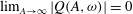 $\lim _{A\rightarrow \infty }|Q(A,\unicode[STIX]{x1D714})|=0$
.
$\lim _{A\rightarrow \infty }|Q(A,\unicode[STIX]{x1D714})|=0$
.
2.3 Governing equations
Making a zero Mach number assumption, the inhomogeneous wave equation governing the problem is, as derived for example by Nicoud et al. (Reference Nicoud, Benoit, Sensiau and Poinsot2007):
 $$\begin{eqnarray}\unicode[STIX]{x1D735}\boldsymbol{\cdot }\left(\frac{1}{\unicode[STIX]{x1D70C}_{0}}\unicode[STIX]{x1D735}p_{1}\right)-\frac{1}{\unicode[STIX]{x1D6FE}p_{0}}\frac{\unicode[STIX]{x2202}^{2}p_{1}}{\unicode[STIX]{x2202}t^{2}}=-\frac{\unicode[STIX]{x1D6FE}-1}{\unicode[STIX]{x1D6FE}p_{0}}\frac{\unicode[STIX]{x2202}q_{1}}{\unicode[STIX]{x2202}t}.\end{eqnarray}$$
In the equation, subscript 0 refers to mean quantities, which depend on
 $\boldsymbol{x}$
only, while subscript 1 refers to fluctuating quantities, which depend on
$\boldsymbol{x}$
only, while subscript 1 refers to fluctuating quantities, which depend on
 $\boldsymbol{x}$
and
$\boldsymbol{x}$
and
 $t$
. In this paper we assume that the density
$t$
. In this paper we assume that the density
 $\unicode[STIX]{x1D70C}_{0}$
and the isentropic coefficient
$\unicode[STIX]{x1D70C}_{0}$
and the isentropic coefficient
 $\unicode[STIX]{x1D6FE}$
are uniform. This hypothesis can possibly be lifted, but the equations become complicated without adding more insight. We also non-dimensionalize the equations, with respect to a spatial length scale
$\unicode[STIX]{x1D6FE}$
are uniform. This hypothesis can possibly be lifted, but the equations become complicated without adding more insight. We also non-dimensionalize the equations, with respect to a spatial length scale
 $D$
(say the radius of the annular chamber) and the acoustic time scale
$D$
(say the radius of the annular chamber) and the acoustic time scale
 $D/c$
, with
$D/c$
, with
 $c$
being the mean speed of sound in the chamber. We assume an ideal gas, so that
$c$
being the mean speed of sound in the chamber. We assume an ideal gas, so that
 $\unicode[STIX]{x1D70C}_{0}c^{2}=\unicode[STIX]{x1D6FE}p_{0}$
. We introduce the non-dimensional fluctuating pressure
$\unicode[STIX]{x1D70C}_{0}c^{2}=\unicode[STIX]{x1D6FE}p_{0}$
. We introduce the non-dimensional fluctuating pressure
 $p$
and fluctuating heat release rate
$p$
and fluctuating heat release rate
 $q$
as
$q$
as
 $$\begin{eqnarray}p\equiv \frac{p_{1}}{\unicode[STIX]{x1D70C}_{0}c^{2}},\quad q\equiv q_{1}\frac{\unicode[STIX]{x1D6FE}-1}{\unicode[STIX]{x1D6FE}p_{0}}\frac{D}{c}.\end{eqnarray}$$
In the new non-dimensional coordinates, equation (2.7) simplifies to
 $$\begin{eqnarray}\frac{\unicode[STIX]{x2202}^{2}p}{\unicode[STIX]{x2202}t^{2}}-\unicode[STIX]{x1D6FB}^{2}p=\mathop{\sum }_{j=1}^{N_{b}}\unicode[STIX]{x1D6FF}(\boldsymbol{x}-\boldsymbol{x}_{j})\frac{\unicode[STIX]{x2202}{\mathcal{Q}}[p_{j}]}{\unicode[STIX]{x2202}t},\end{eqnarray}$$
where we substituted the expression (2.1) and (2.3) for the fluctuating heat release rate
 $q$
. We adopt the following convention for the definition of the Fourier transform:
$q$
. We adopt the following convention for the definition of the Fourier transform:
 $$\begin{eqnarray}\hat{f}(\unicode[STIX]{x1D714})\equiv \frac{1}{\unicode[STIX]{x03C0}}\int _{-\infty }^{\infty }f(t)\text{e}^{-\text{i}\unicode[STIX]{x1D714}t}\,\text{d}t,\quad f(t)=\frac{1}{2}\int _{-\infty }^{\infty }\hat{f}(\unicode[STIX]{x1D714})\text{e}^{+\text{i}\unicode[STIX]{x1D714}t}\,\text{d}\unicode[STIX]{x1D714}.\end{eqnarray}$$
By multiplying all terms of (2.9) by
 $\text{e}^{-\text{i}\unicode[STIX]{x1D714}t}/\unicode[STIX]{x03C0}$
and integrating over the time
$\text{e}^{-\text{i}\unicode[STIX]{x1D714}t}/\unicode[STIX]{x03C0}$
and integrating over the time
 $t$
we obtain the inhomogeneous Helmholtz equation:
$t$
we obtain the inhomogeneous Helmholtz equation:
 $$\begin{eqnarray}\unicode[STIX]{x1D714}^{2}\hat{p}(\boldsymbol{x},\unicode[STIX]{x1D714})+\unicode[STIX]{x1D6FB}^{2}\hat{p}(\boldsymbol{x},\unicode[STIX]{x1D714})=-\mathop{\sum }_{j=1}^{N_{b}}\unicode[STIX]{x1D6FF}(\boldsymbol{x}-\boldsymbol{x}_{j})\frac{1}{\unicode[STIX]{x03C0}}\int _{-\infty }^{\infty }\frac{\unicode[STIX]{x2202}{\mathcal{Q}}[p(\boldsymbol{x}_{j},t)]}{\unicode[STIX]{x2202}t}\text{e}^{-\text{i}\unicode[STIX]{x1D714}t}\,\text{d}t.\end{eqnarray}$$
Each of the integrals in the sum on the right-hand side can be rewritten as
 $$\begin{eqnarray}\displaystyle \frac{1}{\unicode[STIX]{x03C0}}\int _{-\infty }^{\infty }\frac{\unicode[STIX]{x2202}{\mathcal{Q}}[p(\boldsymbol{x}_{j},t)]}{\unicode[STIX]{x2202}t}\text{e}^{-\text{i}\unicode[STIX]{x1D714}t}\,\text{d}t & = & \displaystyle +\text{i}\unicode[STIX]{x1D714}\frac{1}{\unicode[STIX]{x03C0}}\int _{-\infty }^{\infty }{\mathcal{Q}}[p(\boldsymbol{x}_{j},t)]\text{e}^{-\text{i}\unicode[STIX]{x1D714}t}\,\text{d}t\nonumber\\ \displaystyle & = & \displaystyle +\text{i}\unicode[STIX]{x1D714}Q(|\hat{p}(\boldsymbol{x}_{j})|,\unicode[STIX]{x1D714})^{\ast }\hat{p}(\boldsymbol{x}_{j},\unicode[STIX]{x1D714}).\end{eqnarray}$$
Notice that we assume that the response at the frequency
 $\unicode[STIX]{x1D714}$
of
$\unicode[STIX]{x1D714}$
of
 ${\mathcal{Q}}[p(\boldsymbol{x},t)]$
only depends on the amplitude
${\mathcal{Q}}[p(\boldsymbol{x},t)]$
only depends on the amplitude
 $|\hat{p}(\boldsymbol{x})|$
of the solution at the same frequency
$|\hat{p}(\boldsymbol{x})|$
of the solution at the same frequency
 $\unicode[STIX]{x1D714}$
. This is correct as long as all other harmonics are negligible, i.e. the filtering hypothesis holds (Gelb & Vander Velde Reference Gelb and Vander Velde1968). We also point out that in the last passage of (2.12) the complex conjugation denoted by the asterisk appears because of the different sign convention in the exponential in the definitions (2.4) and (2.10). Substituting (2.12) in (2.11) we obtain:
$\unicode[STIX]{x1D714}$
. This is correct as long as all other harmonics are negligible, i.e. the filtering hypothesis holds (Gelb & Vander Velde Reference Gelb and Vander Velde1968). We also point out that in the last passage of (2.12) the complex conjugation denoted by the asterisk appears because of the different sign convention in the exponential in the definitions (2.4) and (2.10). Substituting (2.12) in (2.11) we obtain:
 $$\begin{eqnarray}\unicode[STIX]{x1D714}^{2}\hat{p}(\boldsymbol{x},\unicode[STIX]{x1D714})+\unicode[STIX]{x1D6FB}^{2}\hat{p}(\boldsymbol{x},\unicode[STIX]{x1D714})=-\text{i}\unicode[STIX]{x1D714}\mathop{\sum }_{j=1}^{N_{b}}\unicode[STIX]{x1D6FF}(\boldsymbol{x}-\boldsymbol{x}_{j})Q(|\hat{p}(\boldsymbol{x}_{j})|,\unicode[STIX]{x1D714})^{\ast }\hat{p}(\boldsymbol{x}_{j},\unicode[STIX]{x1D714}).\end{eqnarray}$$
Equation (2.13) must be accompanied by suitable boundary conditions. At the combustor walls these will be zero normal gradient conditions for the pressure. At the axial extremes of the domain, the combustor inlet and outlet, the boundary conditions will in general be of impedance type,
 $\hat{p}=Z(\unicode[STIX]{x1D714})\hat{u}$
, with
$\hat{p}=Z(\unicode[STIX]{x1D714})\hat{u}$
, with
 $Z(\unicode[STIX]{x1D714})$
a complex-valued function.
$Z(\unicode[STIX]{x1D714})$
a complex-valued function.
2.4 Eigenmodes’ degeneracy
We linearise equation (2.13) with respect to the amplitude
 $|\hat{p}(\boldsymbol{x})|$
of the solution and obtain:
$|\hat{p}(\boldsymbol{x})|$
of the solution and obtain:
 $$\begin{eqnarray}\unicode[STIX]{x1D714}^{2}\hat{p}(\boldsymbol{x},\unicode[STIX]{x1D714})+\unicode[STIX]{x1D6FB}^{2}\hat{p}(\boldsymbol{x},\unicode[STIX]{x1D714})=-\text{i}\unicode[STIX]{x1D714}\mathop{\sum }_{j=1}^{N_{b}}\unicode[STIX]{x1D6FF}(\boldsymbol{x}-\boldsymbol{x}_{j})L(\unicode[STIX]{x1D714})\hat{p}(\boldsymbol{x}_{j},\unicode[STIX]{x1D714}),\end{eqnarray}$$
where
 $L(\unicode[STIX]{x1D714})$
is the transfer function of
$L(\unicode[STIX]{x1D714})$
is the transfer function of
 ${\mathcal{Q}}[p(t)]$
at infinitesimal amplitudes. The set of solutions of the eigenvalue problem (2.14) is
${\mathcal{Q}}[p(t)]$
at infinitesimal amplitudes. The set of solutions of the eigenvalue problem (2.14) is
 $\{(\hat{\unicode[STIX]{x1D713}}_{n}(\boldsymbol{x}),\unicode[STIX]{x1D70E}_{n}+\text{i}\hat{\unicode[STIX]{x1D714}}_{n})$
with
$\{(\hat{\unicode[STIX]{x1D713}}_{n}(\boldsymbol{x}),\unicode[STIX]{x1D70E}_{n}+\text{i}\hat{\unicode[STIX]{x1D714}}_{n})$
with
 $\,\,\unicode[STIX]{x1D70E}_{n},\hat{\unicode[STIX]{x1D714}}_{n}\in \mathbb{R}\,\,,n=1,2,\ldots \}$
where
$\,\,\unicode[STIX]{x1D70E}_{n},\hat{\unicode[STIX]{x1D714}}_{n}\in \mathbb{R}\,\,,n=1,2,\ldots \}$
where
 $\hat{\unicode[STIX]{x1D713}}_{n}(\boldsymbol{x})$
is the complex-valued eigenvector describing the shape of the mode and
$\hat{\unicode[STIX]{x1D713}}_{n}(\boldsymbol{x})$
is the complex-valued eigenvector describing the shape of the mode and
 $\unicode[STIX]{x1D70E}_{n}+\text{i}\hat{\unicode[STIX]{x1D714}}_{n}$
is the corresponding eigenvalue. The modes and their eigenvalues can be calculated using a Helmholtz solver (Nicoud et al.
Reference Nicoud, Benoit, Sensiau and Poinsot2007) or a thermoacoustic network model of the problem (Stow & Dowling Reference Stow and Dowling2001; Schuermans, Bellucci & Paschereit Reference Schuermans, Bellucci and Paschereit2003).
$\unicode[STIX]{x1D70E}_{n}+\text{i}\hat{\unicode[STIX]{x1D714}}_{n}$
is the corresponding eigenvalue. The modes and their eigenvalues can be calculated using a Helmholtz solver (Nicoud et al.
Reference Nicoud, Benoit, Sensiau and Poinsot2007) or a thermoacoustic network model of the problem (Stow & Dowling Reference Stow and Dowling2001; Schuermans, Bellucci & Paschereit Reference Schuermans, Bellucci and Paschereit2003).
We are particularly interested in azimuthal modes, i.e. solutions that are
 $n$
-periodic in
$n$
-periodic in
 $\unicode[STIX]{x1D703}$
in
$\unicode[STIX]{x1D703}$
in
 $[0\,,\,2\unicode[STIX]{x03C0}]$
, with
$[0\,,\,2\unicode[STIX]{x03C0}]$
, with
 $n$
called the azimuthal wavenumber of the mode. As discussed by Moeck, Paul & Paschereit (Reference Moeck, Paul and Paschereit2010), Bauerheim et al. (Reference Bauerheim, Salas, Nicoud and Poinsot2014), an azimuthal mode of wavenumber
$n$
called the azimuthal wavenumber of the mode. As discussed by Moeck, Paul & Paschereit (Reference Moeck, Paul and Paschereit2010), Bauerheim et al. (Reference Bauerheim, Salas, Nicoud and Poinsot2014), an azimuthal mode of wavenumber
 $n$
belongs to an eigenspace of dimension two because of the rotational symmetry of the problem. There are however exceptions, when
$n$
belongs to an eigenspace of dimension two because of the rotational symmetry of the problem. There are however exceptions, when
 $n$
is a multiple of
$n$
is a multiple of
 $N_{b}/2$
in the case of an even number of burners
$N_{b}/2$
in the case of an even number of burners
 $N_{b}$
, and when
$N_{b}$
, and when
 $n$
is a multiple of
$n$
is a multiple of
 $N_{b}$
in the case of
$N_{b}$
in the case of
 $N_{b}$
odd. We refer the reader also to § 5.4 of Salas (Reference Salas2013) for a concise summary of these two cases. These exceptions are non-degenerate cases, i.e. their modes belong to an eigenspace of dimension one, and occur because the rotational symmetry is discrete. We focus the analysis on the degenerate case where the dimensionality is two because: (i)
$N_{b}$
odd. We refer the reader also to § 5.4 of Salas (Reference Salas2013) for a concise summary of these two cases. These exceptions are non-degenerate cases, i.e. their modes belong to an eigenspace of dimension one, and occur because the rotational symmetry is discrete. We focus the analysis on the degenerate case where the dimensionality is two because: (i)
 $N_{b}$
is usually large and the excited modes typically have a low azimuthal wavenumber
$N_{b}$
is usually large and the excited modes typically have a low azimuthal wavenumber
 $n$
(up to
$n$
(up to
 $n=4$
in Seume et al. (Reference Seume, Vortmeyer, Krause, Hermann, Hantschk, Gleis, Vortmeyer and Orthmann1998)); (ii) the non-degenerate case does not give rise to the rich dynamics that can be observed in the degenerate case. We study thermoacoustic oscillations of azimuthal modes with
$n=4$
in Seume et al. (Reference Seume, Vortmeyer, Krause, Hermann, Hantschk, Gleis, Vortmeyer and Orthmann1998)); (ii) the non-degenerate case does not give rise to the rich dynamics that can be observed in the degenerate case. We study thermoacoustic oscillations of azimuthal modes with
 $n=1$
in the following, but the same analysis can be generalized to higher
$n=1$
in the following, but the same analysis can be generalized to higher
 $n$
, as long as the case stays degenerate.
$n$
, as long as the case stays degenerate.
We assume that these modes are close to their Hopf bifurcation. In other words, we assume that all other modes are stable, and only azimuthal modes of wavenumber
 $n=1$
take part in the oscillation. The Floquet–Bloch theorem (Chap. VIII pp. 139–140 Brillouin Reference Brillouin1953; Mensah & Moeck Reference Mensah and Moeck2015) ensures that one of the
$n=1$
take part in the oscillation. The Floquet–Bloch theorem (Chap. VIII pp. 139–140 Brillouin Reference Brillouin1953; Mensah & Moeck Reference Mensah and Moeck2015) ensures that one of the
 $n=1$
solutions can generally be written in the form
$n=1$
solutions can generally be written in the form
 $\widetilde{\unicode[STIX]{x1D712}}(z,r)\text{e}^{\text{i}\unicode[STIX]{x1D703}}$
, where
$\widetilde{\unicode[STIX]{x1D712}}(z,r)\text{e}^{\text{i}\unicode[STIX]{x1D703}}$
, where
 $\widetilde{\unicode[STIX]{x1D712}}(z,r)$
is periodic in
$\widetilde{\unicode[STIX]{x1D712}}(z,r)$
is periodic in
 $\unicode[STIX]{x1D703}$
with period
$\unicode[STIX]{x1D703}$
with period
 $2\unicode[STIX]{x03C0}/N_{b}$
, i.e. one burner segment. The dependence of
$2\unicode[STIX]{x03C0}/N_{b}$
, i.e. one burner segment. The dependence of
 $\unicode[STIX]{x1D712}$
on
$\unicode[STIX]{x1D712}$
on
 $\unicode[STIX]{x1D703}$
can be in principle be taken into account. Since it is of secondary importance when compared to the long-wave component
$\unicode[STIX]{x1D703}$
can be in principle be taken into account. Since it is of secondary importance when compared to the long-wave component
 $\text{e}^{\text{i}\unicode[STIX]{x1D703}}$
, it is neglected in the following in favour of a clearer exposition. Because of the reflection symmetry of the problem, there exists a second solution of the eigenspace that is symmetric with respect to the first, with structure
$\text{e}^{\text{i}\unicode[STIX]{x1D703}}$
, it is neglected in the following in favour of a clearer exposition. Because of the reflection symmetry of the problem, there exists a second solution of the eigenspace that is symmetric with respect to the first, with structure
 $\widetilde{\unicode[STIX]{x1D712}}(z,r)\text{e}^{-\text{i}\unicode[STIX]{x1D703}}$
. We refer to these two modes in the following as spinning modes, because their phases linearly increase or decrease in the azimuthal direction.
$\widetilde{\unicode[STIX]{x1D712}}(z,r)\text{e}^{-\text{i}\unicode[STIX]{x1D703}}$
. We refer to these two modes in the following as spinning modes, because their phases linearly increase or decrease in the azimuthal direction.
By linearly combining these two spinning modes we can obtain two solutions
 $\unicode[STIX]{x1D713}_{1}$
and
$\unicode[STIX]{x1D713}_{1}$
and
 $\unicode[STIX]{x1D713}_{2}$
that have a constant phase as a function of
$\unicode[STIX]{x1D713}_{2}$
that have a constant phase as a function of
 $\unicode[STIX]{x1D703}$
:
$\unicode[STIX]{x1D703}$
:
 $$\begin{eqnarray}\displaystyle & \displaystyle \widetilde{\unicode[STIX]{x1D713}}_{1}(\boldsymbol{x})={\textstyle \frac{1}{2}}\left[\widetilde{\unicode[STIX]{x1D712}}(z,r)\text{e}^{\text{i}\unicode[STIX]{x1D703}}+\widetilde{\unicode[STIX]{x1D712}}(z,r)\text{e}^{-\text{i}\unicode[STIX]{x1D703}}\right]=\widetilde{\unicode[STIX]{x1D712}}(z,r)\cos (\unicode[STIX]{x1D703}), & \displaystyle\end{eqnarray}$$
 $$\begin{eqnarray}\displaystyle & \displaystyle \widetilde{\unicode[STIX]{x1D713}}_{2}(\boldsymbol{x})=\frac{1}{2i}\left[\widetilde{\unicode[STIX]{x1D712}}(z,r)\text{e}^{\text{i}\unicode[STIX]{x1D703}}-\widetilde{\unicode[STIX]{x1D712}}(z,r)\text{e}^{-\text{i}\unicode[STIX]{x1D703}}\right]=\widetilde{\unicode[STIX]{x1D712}}(z,r)\sin (\unicode[STIX]{x1D703}). & \displaystyle\end{eqnarray}$$
 $$\begin{eqnarray}\int _{\unicode[STIX]{x1D6FA}}\widetilde{\unicode[STIX]{x1D713}}_{1}(\boldsymbol{x})\widetilde{\unicode[STIX]{x1D713}}_{2}(\boldsymbol{x})^{\ast }\,\text{d}\unicode[STIX]{x1D6FA}=0,\end{eqnarray}$$
where
 $\unicode[STIX]{x1D6FA}$
is the volume of the combustion chamber. One proves by direct substitution also that
$\unicode[STIX]{x1D6FA}$
is the volume of the combustion chamber. One proves by direct substitution also that
 $$\begin{eqnarray}\int _{\unicode[STIX]{x1D6FA}}\widetilde{\unicode[STIX]{x1D713}}_{1}^{\ast }\unicode[STIX]{x1D6FB}^{2}\widetilde{\unicode[STIX]{x1D713}}_{2}\,\text{d}\unicode[STIX]{x1D6FA}=\int _{\unicode[STIX]{x1D6FA}}\widetilde{\unicode[STIX]{x1D713}}_{2}^{\ast }\unicode[STIX]{x1D6FB}^{2}\widetilde{\unicode[STIX]{x1D713}}_{1}\,\text{d}\unicode[STIX]{x1D6FA}=0.\end{eqnarray}$$
We normalise the standing modes by fixing the value of
 $\widetilde{\unicode[STIX]{x1D712}}(0,\overline{r})$
to 1 at the burners’ positions
$\widetilde{\unicode[STIX]{x1D712}}(0,\overline{r})$
to 1 at the burners’ positions
 $(z,r,\unicode[STIX]{x1D703})=(0,\overline{r},\unicode[STIX]{x1D703}_{j})$
, so that
$(z,r,\unicode[STIX]{x1D703})=(0,\overline{r},\unicode[STIX]{x1D703}_{j})$
, so that
 $$\begin{eqnarray}\left\{\begin{array}{@{}l@{}}\widetilde{\unicode[STIX]{x1D713}}_{1}(\boldsymbol{x}_{j})=\widetilde{\unicode[STIX]{x1D713}}_{1}(0,\overline{r},\unicode[STIX]{x1D703}_{j})=c_{j},\quad \\ \widetilde{\unicode[STIX]{x1D713}}_{2}(\boldsymbol{x}_{j})=\widetilde{\unicode[STIX]{x1D713}}_{2}(0,\overline{r},\unicode[STIX]{x1D703}_{j})=s_{j},\quad \end{array}\right.\text{with the notation: }\left\{\begin{array}{@{}l@{}}c_{j}\equiv \cos (\unicode[STIX]{x1D703}_{j}),\quad \\ s_{j}\equiv \sin (\unicode[STIX]{x1D703}_{j}).\quad \end{array}\right.\end{eqnarray}$$
2.5 Weakly nonlinear analysis
We study the solution of the nonlinear problem as a perturbation of its linear, neutrally stable counterpart. We obtain the latter by changing the problem (2.14), by substituting
 $\widetilde{\unicode[STIX]{x1D709}}L(\unicode[STIX]{x1D714})$
in place of
$\widetilde{\unicode[STIX]{x1D709}}L(\unicode[STIX]{x1D714})$
in place of
 $L(\unicode[STIX]{x1D714})$
, with
$L(\unicode[STIX]{x1D714})$
, with
 $\widetilde{\unicode[STIX]{x1D709}}$
a real, non-negative coefficient, so that for
$\widetilde{\unicode[STIX]{x1D709}}$
a real, non-negative coefficient, so that for
 $\widetilde{\unicode[STIX]{x1D709}}=1$
we recover the original equations. We then look for the value
$\widetilde{\unicode[STIX]{x1D709}}=1$
we recover the original equations. We then look for the value
 $\unicode[STIX]{x1D709}$
of the coefficient
$\unicode[STIX]{x1D709}$
of the coefficient
 $\widetilde{\unicode[STIX]{x1D709}}$
such that the growth rate of the first two modes
$\widetilde{\unicode[STIX]{x1D709}}$
such that the growth rate of the first two modes
 $\unicode[STIX]{x1D70E}_{1,2}(\widetilde{\unicode[STIX]{x1D709}})$
is zero. In other words, we linearly increase/decrease the gain of the flame response to the level that makes the system neutrally stable. Notice that by looking at (2.14), one may guess that this may happen only for
$\unicode[STIX]{x1D70E}_{1,2}(\widetilde{\unicode[STIX]{x1D709}})$
is zero. In other words, we linearly increase/decrease the gain of the flame response to the level that makes the system neutrally stable. Notice that by looking at (2.14), one may guess that this may happen only for
 $\widetilde{\unicode[STIX]{x1D709}}=0$
. This is not generally the case, due to the presence of partially transmitting boundary conditions or sources of damping, such as Helmholtz resonators and/or acoustic liners that remove fluctuation energy from the system. In this study, we consider only linear damping. Nonlinear acoustic damping effects at the boundaries can be characterised with a describing function (Schuller et al.
Reference Schuller, Tran, Noiray, Durox, Ducruix and Candel2009) in the frequency domain, and its time-domain realization (Ghirardo et al.
Reference Ghirardo, Ćosić, Juniper and Moeck2015) in the time domain. We refer to quantities evaluated for
$\widetilde{\unicode[STIX]{x1D709}}=0$
. This is not generally the case, due to the presence of partially transmitting boundary conditions or sources of damping, such as Helmholtz resonators and/or acoustic liners that remove fluctuation energy from the system. In this study, we consider only linear damping. Nonlinear acoustic damping effects at the boundaries can be characterised with a describing function (Schuller et al.
Reference Schuller, Tran, Noiray, Durox, Ducruix and Candel2009) in the frequency domain, and its time-domain realization (Ghirardo et al.
Reference Ghirardo, Ćosić, Juniper and Moeck2015) in the time domain. We refer to quantities evaluated for
 $\widetilde{\unicode[STIX]{x1D709}}=\unicode[STIX]{x1D709}$
by dropping the tilde, so that the eigenmodes are indicated with
$\widetilde{\unicode[STIX]{x1D709}}=\unicode[STIX]{x1D709}$
by dropping the tilde, so that the eigenmodes are indicated with
 $\unicode[STIX]{x1D713}_{1}(\boldsymbol{x})$
and
$\unicode[STIX]{x1D713}_{1}(\boldsymbol{x})$
and
 $\unicode[STIX]{x1D713}_{2}(\boldsymbol{x})$
, and their real-valued eigenfrequency is
$\unicode[STIX]{x1D713}_{2}(\boldsymbol{x})$
, and their real-valued eigenfrequency is
 $\unicode[STIX]{x1D714}_{1}=\unicode[STIX]{x1D714}_{2}$
.
$\unicode[STIX]{x1D714}_{1}=\unicode[STIX]{x1D714}_{2}$
.
For later use, we write (2.14) for the first two modes to obtain
 $$\begin{eqnarray}\displaystyle \unicode[STIX]{x1D6FB}^{2}[\unicode[STIX]{x1D713}_{k}(\boldsymbol{x})] & = & \displaystyle -[\unicode[STIX]{x1D714}_{k}^{2}\unicode[STIX]{x1D713}_{k}(\boldsymbol{x})-\mathop{\sum }_{j=1}^{N_{b}}\unicode[STIX]{x1D6FF}(\boldsymbol{x}-\boldsymbol{x}_{j})\unicode[STIX]{x1D714}_{k}\unicode[STIX]{x1D709}\,\text{Im}\left[L(\unicode[STIX]{x1D714}_{k})\right]\unicode[STIX]{x1D713}_{k}(\boldsymbol{x}_{j})]\nonumber\\ \displaystyle & & \displaystyle -\,\cdots \text{i}\mathop{\sum }_{j=1}^{N_{b}}\unicode[STIX]{x1D6FF}(\boldsymbol{x}-\boldsymbol{x}_{j})\unicode[STIX]{x1D714}_{k}\unicode[STIX]{x1D709}\,\text{Re}[L(\unicode[STIX]{x1D714}_{k})]\unicode[STIX]{x1D713}_{k}(\boldsymbol{x}_{j}),\quad k=1,2,\quad \unicode[STIX]{x1D714}_{1}=\unicode[STIX]{x1D714}_{2}.\qquad\end{eqnarray}$$
We can multiply all terms of (2.18) by
 $\unicode[STIX]{x1D713}_{k}^{\ast }$
and integrate over the domain
$\unicode[STIX]{x1D713}_{k}^{\ast }$
and integrate over the domain
 $\unicode[STIX]{x1D6FA}$
:
$\unicode[STIX]{x1D6FA}$
:
 $$\begin{eqnarray}\int _{\unicode[STIX]{x1D6FA}}\unicode[STIX]{x1D6FB}^{2}\unicode[STIX]{x1D713}_{k}\unicode[STIX]{x1D713}_{k}^{\ast }\,\text{d}\unicode[STIX]{x1D6FA}=-[\unicode[STIX]{x1D714}_{0}^{2}+\text{i}\unicode[STIX]{x1D714}_{k}\unicode[STIX]{x1D6FC}]\int _{\unicode[STIX]{x1D6FA}}\unicode[STIX]{x1D713}_{k}\unicode[STIX]{x1D713}_{k}^{\ast }\,\text{d}\unicode[STIX]{x1D6FA},\quad k=1,2,\end{eqnarray}$$
where, by exploiting the fact that
 $\sum _{j=1}^{N_{b}}c_{j}^{2}=\sum _{j=1}^{N_{b}}s_{j}^{2}=N_{b}/2$
, we introduced the quantities
$\sum _{j=1}^{N_{b}}c_{j}^{2}=\sum _{j=1}^{N_{b}}s_{j}^{2}=N_{b}/2$
, we introduced the quantities
 $$\begin{eqnarray}\displaystyle & \displaystyle \unicode[STIX]{x1D714}_{0}^{2}\equiv \unicode[STIX]{x1D714}_{k}^{2}-\unicode[STIX]{x1D714}_{k}\unicode[STIX]{x1D709}\,\text{Im}[L(\unicode[STIX]{x1D714}_{k})]\unicode[STIX]{x1D707}\mathop{\sum }_{j=1}^{N_{b}}|\unicode[STIX]{x1D713}_{k}(\boldsymbol{x}_{j})|^{2}=\unicode[STIX]{x1D714}_{k}^{2}-\unicode[STIX]{x1D714}_{k}\unicode[STIX]{x1D709}\,\text{Im}[L(\unicode[STIX]{x1D714}_{k})]\unicode[STIX]{x1D707}\frac{N_{b}}{2}, & \displaystyle\end{eqnarray}$$
 $$\begin{eqnarray}\displaystyle & \displaystyle \unicode[STIX]{x1D6FC}\equiv \unicode[STIX]{x1D709}\,\text{Re}[L(\unicode[STIX]{x1D714}_{k})]\unicode[STIX]{x1D707}\mathop{\sum }_{j=1}^{N_{b}}|\unicode[STIX]{x1D713}_{k}(\boldsymbol{x}_{j})|^{2}=\unicode[STIX]{x1D709}\,\text{Re}[L(\unicode[STIX]{x1D714}_{n})]\unicode[STIX]{x1D707}\frac{N_{b}}{2}, & \displaystyle\end{eqnarray}$$
 $\unicode[STIX]{x1D707}=\unicode[STIX]{x1D707}_{1}=\unicode[STIX]{x1D707}_{2}$
is a real valued normalisation factor that is the same for the two modes, defined as:
$\unicode[STIX]{x1D707}=\unicode[STIX]{x1D707}_{1}=\unicode[STIX]{x1D707}_{2}$
is a real valued normalisation factor that is the same for the two modes, defined as:  $$\begin{eqnarray}\unicode[STIX]{x1D707}=\frac{1}{\displaystyle \int _{\unicode[STIX]{x1D6FA}}\unicode[STIX]{x1D713}_{1}\unicode[STIX]{x1D713}_{1}^{\ast }\,\text{d}\unicode[STIX]{x1D6FA}}.\end{eqnarray}$$
In both right-hand sides of (2.20) the frequency
 $\unicode[STIX]{x1D714}_{k}=\unicode[STIX]{x1D714}_{1}=\unicode[STIX]{x1D714}_{2}$
is much larger than the other terms, so that
$\unicode[STIX]{x1D714}_{k}=\unicode[STIX]{x1D714}_{1}=\unicode[STIX]{x1D714}_{2}$
is much larger than the other terms, so that
 $\unicode[STIX]{x1D714}_{0}\approx \unicode[STIX]{x1D714}_{k}$
and
$\unicode[STIX]{x1D714}_{0}\approx \unicode[STIX]{x1D714}_{k}$
and
 $\unicode[STIX]{x1D6FC}\ll |\unicode[STIX]{x1D714}_{k}|$
. This follows from the weakly nonlinear nature of thermoacoustic problems. Equations (2.20) define the equivalent acoustic damping
$\unicode[STIX]{x1D6FC}\ll |\unicode[STIX]{x1D714}_{k}|$
. This follows from the weakly nonlinear nature of thermoacoustic problems. Equations (2.20) define the equivalent acoustic damping
 $\unicode[STIX]{x1D6FC}$
and natural frequency
$\unicode[STIX]{x1D6FC}$
and natural frequency
 $\unicode[STIX]{x1D714}_{0}$
of the system when the flame response is uniformly reduced in the annulus to the point of making the system neutrally stable, i.e. at
$\unicode[STIX]{x1D714}_{0}$
of the system when the flame response is uniformly reduced in the annulus to the point of making the system neutrally stable, i.e. at
 $\widetilde{\unicode[STIX]{x1D709}}=\unicode[STIX]{x1D709}$
. This paragraph led to (2.19), which will be used in the following.
$\widetilde{\unicode[STIX]{x1D709}}=\unicode[STIX]{x1D709}$
. This paragraph led to (2.19), which will be used in the following.
At the value
 $\widetilde{\unicode[STIX]{x1D709}}=\unicode[STIX]{x1D709}$
no dissipation/gain of energy in a limit cycle occurs in the linearised system for the dominant mode, and the exact solution of the problem is
$\widetilde{\unicode[STIX]{x1D709}}=\unicode[STIX]{x1D709}$
no dissipation/gain of energy in a limit cycle occurs in the linearised system for the dominant mode, and the exact solution of the problem is
 $$\begin{eqnarray}p(\boldsymbol{x},t)=[X_{1}\unicode[STIX]{x1D713}_{1}(\boldsymbol{x})\text{e}^{\text{i}(\unicode[STIX]{x1D714}_{1}t+\unicode[STIX]{x1D711}_{1})}+X_{2}\unicode[STIX]{x1D713}_{2}(\boldsymbol{x})\text{e}^{\text{i}(\unicode[STIX]{x1D714}_{1}t+\unicode[STIX]{x1D711}_{2})}+\text{c.c.}]+\text{decaying terms},\end{eqnarray}$$
where
 $X_{1}$
and
$X_{1}$
and
 $X_{2}$
are two complex-valued constants and the decaying terms depend on the initial condition and they will be neglected in the following because they converge to zero in time after the initial transient. We now study the original nonlinear problem (2.9) as a perturbation of this, as
$X_{2}$
are two complex-valued constants and the decaying terms depend on the initial condition and they will be neglected in the following because they converge to zero in time after the initial transient. We now study the original nonlinear problem (2.9) as a perturbation of this, as
 $\widetilde{\unicode[STIX]{x1D709}}$
changes from
$\widetilde{\unicode[STIX]{x1D709}}$
changes from
 $\unicode[STIX]{x1D709}$
to 1. We choose as ansatz in the frequency domain
$\unicode[STIX]{x1D709}$
to 1. We choose as ansatz in the frequency domain
 $$\begin{eqnarray}\hat{p}(\boldsymbol{x},\unicode[STIX]{x1D714})=\text{i}\unicode[STIX]{x1D714}[\hat{\unicode[STIX]{x1D702}}_{1}(\unicode[STIX]{x1D714})\unicode[STIX]{x1D713}_{1}(\boldsymbol{x})+\hat{\unicode[STIX]{x1D702}}_{2}(\unicode[STIX]{x1D714})\unicode[STIX]{x1D713}_{2}(\boldsymbol{x})]+\unicode[STIX]{x1D700}\hat{p}_{\unicode[STIX]{x1D700}}(\boldsymbol{x},\unicode[STIX]{x1D714}).\end{eqnarray}$$
In (2.23),
 $\unicode[STIX]{x1D700}=1-\unicode[STIX]{x1D709}$
is the perturbation parameter and expresses the deviation of the exact nonlinear solution from the first term at the right-hand side, which is the solution of the linear problem, with coefficients
$\unicode[STIX]{x1D700}=1-\unicode[STIX]{x1D709}$
is the perturbation parameter and expresses the deviation of the exact nonlinear solution from the first term at the right-hand side, which is the solution of the linear problem, with coefficients
 $\hat{\unicode[STIX]{x1D702}}_{k}$
that will be calculated next. This deviation occurs because of the onset of higher harmonics in time and in space, and because of the structural change in the equations that can affect slightly the shape of the modes. Using (2.17), the expression for the pressure field at the burners’ location reads
$\hat{\unicode[STIX]{x1D702}}_{k}$
that will be calculated next. This deviation occurs because of the onset of higher harmonics in time and in space, and because of the structural change in the equations that can affect slightly the shape of the modes. Using (2.17), the expression for the pressure field at the burners’ location reads
 $$\begin{eqnarray}\hat{p}(\boldsymbol{x}_{j},\unicode[STIX]{x1D714})=[\text{i}\unicode[STIX]{x1D714}\hat{\unicode[STIX]{x1D702}}_{1}(\unicode[STIX]{x1D714})c_{j}+\text{i}\unicode[STIX]{x1D714}\hat{\unicode[STIX]{x1D702}}_{2}(\unicode[STIX]{x1D714})s_{j}]+\unicode[STIX]{x1D700}\hat{p}_{\unicode[STIX]{x1D700}}(\boldsymbol{x}_{j},\unicode[STIX]{x1D714}).\end{eqnarray}$$
We then substitute this ansatz into (2.13), multiply all terms by
 $-\unicode[STIX]{x1D713}_{1}(\boldsymbol{x})^{\ast }/(\text{i}\unicode[STIX]{x1D714})$
, and integrate over the domain
$-\unicode[STIX]{x1D713}_{1}(\boldsymbol{x})^{\ast }/(\text{i}\unicode[STIX]{x1D714})$
, and integrate over the domain
 $\unicode[STIX]{x1D6FA}$
. We first exploit the orthogonality properties (2.16) between the two degenerate modes, and then substitute (2.19) and obtain:
$\unicode[STIX]{x1D6FA}$
. We first exploit the orthogonality properties (2.16) between the two degenerate modes, and then substitute (2.19) and obtain:
 $$\begin{eqnarray}\displaystyle & & \displaystyle [-\unicode[STIX]{x1D714}^{2}\hat{\unicode[STIX]{x1D702}}_{1}+\text{i}\unicode[STIX]{x1D714}_{1}\unicode[STIX]{x1D6FC}\hat{\unicode[STIX]{x1D702}}_{1}+\unicode[STIX]{x1D714}_{0}^{2}\hat{\unicode[STIX]{x1D702}}_{1}]\int _{\unicode[STIX]{x1D6FA}}\unicode[STIX]{x1D713}_{1}\unicode[STIX]{x1D713}_{1}^{\ast }\,\text{d}\unicode[STIX]{x1D6FA}\nonumber\\ \displaystyle & & \displaystyle \quad =\cdots \mathop{\sum }_{j=1}^{N_{b}}Q^{\ast }(|\text{i}\unicode[STIX]{x1D714}\hat{\unicode[STIX]{x1D702}}_{1}c_{j}+\text{i}\unicode[STIX]{x1D714}\hat{\unicode[STIX]{x1D702}}_{2}s_{j}|,\unicode[STIX]{x1D714})[\text{i}\unicode[STIX]{x1D714}\hat{\unicode[STIX]{x1D702}}_{1}c_{j}+\text{i}\unicode[STIX]{x1D714}\hat{\unicode[STIX]{x1D702}}_{2}s_{j}]c_{j}+O(\unicode[STIX]{x1D700}).\end{eqnarray}$$
Notice how on the left-hand side, the frequency
 $\unicode[STIX]{x1D714}_{1}$
is the frequency of the mode
$\unicode[STIX]{x1D714}_{1}$
is the frequency of the mode
 $\unicode[STIX]{x1D713}_{1}$
, so that in principle
$\unicode[STIX]{x1D713}_{1}$
, so that in principle
 $\text{i}\unicode[STIX]{x1D714}_{1}\hat{\unicode[STIX]{x1D702}}_{1}$
is not the Fourier transform of
$\text{i}\unicode[STIX]{x1D714}_{1}\hat{\unicode[STIX]{x1D702}}_{1}$
is not the Fourier transform of
 $\unicode[STIX]{x2202}\unicode[STIX]{x1D702}_{1}/\unicode[STIX]{x2202}t$
. However, the frequency of the nonlinear system
$\unicode[STIX]{x2202}\unicode[STIX]{x1D702}_{1}/\unicode[STIX]{x2202}t$
. However, the frequency of the nonlinear system
 $\unicode[STIX]{x1D714}$
is close to
$\unicode[STIX]{x1D714}$
is close to
 $\unicode[STIX]{x1D714}_{1}$
, and we can make this approximation. We take the inverse Fourier transform of all terms and obtain
$\unicode[STIX]{x1D714}_{1}$
, and we can make this approximation. We take the inverse Fourier transform of all terms and obtain
 $$\begin{eqnarray}\displaystyle & \displaystyle \frac{\unicode[STIX]{x2202}^{2}\unicode[STIX]{x1D702}_{1}}{\unicode[STIX]{x2202}t^{2}}+\unicode[STIX]{x1D6FC}\frac{\unicode[STIX]{x2202}\unicode[STIX]{x1D702}_{1}}{\unicode[STIX]{x2202}t}+\unicode[STIX]{x1D714}_{0}^{2}\unicode[STIX]{x1D702}_{1}=\mathop{\sum }_{j=1}^{N_{b}}{\mathcal{Q}}\left[\frac{\unicode[STIX]{x2202}\unicode[STIX]{x1D702}_{1}}{\unicode[STIX]{x2202}t}c_{j}+\frac{\unicode[STIX]{x2202}\unicode[STIX]{x1D702}_{2}}{\unicode[STIX]{x2202}t}s_{j}\right]\unicode[STIX]{x1D707}c_{j}+O(\unicode[STIX]{x1D700}), & \displaystyle\end{eqnarray}$$
 $$\begin{eqnarray}\displaystyle & \displaystyle \frac{\unicode[STIX]{x2202}^{2}\unicode[STIX]{x1D702}_{2}}{\unicode[STIX]{x2202}t^{2}}+\unicode[STIX]{x1D6FC}\frac{\unicode[STIX]{x2202}\unicode[STIX]{x1D702}_{2}}{\unicode[STIX]{x2202}t}+\unicode[STIX]{x1D714}_{0}^{2}\unicode[STIX]{x1D702}_{2}=\mathop{\sum }_{j=1}^{N_{b}}{\mathcal{Q}}\left[\frac{\unicode[STIX]{x2202}\unicode[STIX]{x1D702}_{1}}{\unicode[STIX]{x2202}t}c_{j}+\frac{\unicode[STIX]{x2202}\unicode[STIX]{x1D702}_{2}}{\unicode[STIX]{x2202}t}s_{j}\right]\unicode[STIX]{x1D707}s_{j}+O(\unicode[STIX]{x1D700}), & \displaystyle\end{eqnarray}$$
 $c_{j}$
and
$c_{j}$
and
 $s_{j}$
were introduced in (2.17) and
$s_{j}$
were introduced in (2.17) and
 $\unicode[STIX]{x1D707}$
was defined in (2.21). The equations (2.26) are investigated in the rest of the paper and describe the temporal evolution of the amplitudes
$\unicode[STIX]{x1D707}$
was defined in (2.21). The equations (2.26) are investigated in the rest of the paper and describe the temporal evolution of the amplitudes
 $\unicode[STIX]{x1D702}_{1}(t)$
and
$\unicode[STIX]{x1D702}_{1}(t)$
and
 $\unicode[STIX]{x1D702}_{2}(t)$
of the two standing modes
$\unicode[STIX]{x1D702}_{2}(t)$
of the two standing modes
 $\unicode[STIX]{x1D713}_{1}$
and
$\unicode[STIX]{x1D713}_{1}$
and
 $\unicode[STIX]{x1D713}_{2}$
. The left-hand side of equation (2.26a
) describes a damped oscillator with natural frequency
$\unicode[STIX]{x1D713}_{2}$
. The left-hand side of equation (2.26a
) describes a damped oscillator with natural frequency
 $\unicode[STIX]{x1D714}_{0}$
, defined in (2.20a
), and the damping
$\unicode[STIX]{x1D714}_{0}$
, defined in (2.20a
), and the damping
 $\unicode[STIX]{x1D6FC}$
, defined in (2.20b
). The right-hand side of equation (2.26a
) is the ensemble response of the flames. The argument of the operator
$\unicode[STIX]{x1D6FC}$
, defined in (2.20b
). The right-hand side of equation (2.26a
) is the ensemble response of the flames. The argument of the operator
 ${\mathcal{Q}}$
is the local value of the pressure at the
${\mathcal{Q}}$
is the local value of the pressure at the
 $j$
th burner truncated at zero order, as can be observed in (2.24). Notice how the local contribution of the
$j$
th burner truncated at zero order, as can be observed in (2.24). Notice how the local contribution of the
 $j$
th burner in the sum on the right-hand side is weighted by the term
$j$
th burner in the sum on the right-hand side is weighted by the term
 $\unicode[STIX]{x1D707}c_{j}$
, which is a measure of how large the mode is at that burner.
$\unicode[STIX]{x1D707}c_{j}$
, which is a measure of how large the mode is at that burner.
2.5.1 Linear analysis
In the linear limit, by exploiting the fact that
 $\sum _{j=1}^{N_{b}}c_{j}s_{j}=0$
and that
$\sum _{j=1}^{N_{b}}c_{j}s_{j}=0$
and that
 $\sum _{j=1}^{N_{b}}c_{j}^{2}=N_{b}/2$
, equation (2.26a
) simplifies to:
$\sum _{j=1}^{N_{b}}c_{j}^{2}=N_{b}/2$
, equation (2.26a
) simplifies to:
 $$\begin{eqnarray}\frac{\unicode[STIX]{x2202}^{2}\unicode[STIX]{x1D702}_{1}}{\unicode[STIX]{x2202}t^{2}}+\unicode[STIX]{x1D6FC}\frac{\unicode[STIX]{x2202}\unicode[STIX]{x1D702}_{1}}{\unicode[STIX]{x2202}t}+\unicode[STIX]{x1D714}_{0}^{2}\unicode[STIX]{x1D702}_{1}=\mathop{\sum }_{j=1}^{N_{b}}{\mathcal{L}}\left[\frac{\unicode[STIX]{x2202}\unicode[STIX]{x1D702}_{1}}{\unicode[STIX]{x2202}t}\right]c_{j}^{2}=\unicode[STIX]{x1D707}\frac{N_{b}}{2}{\mathcal{L}}\left[\frac{\unicode[STIX]{x2202}\unicode[STIX]{x1D702}_{1}}{\unicode[STIX]{x2202}t}\right],\end{eqnarray}$$
where
 ${\mathcal{L}}$
is the linearisation of the nonlinear time-domain operator
${\mathcal{L}}$
is the linearisation of the nonlinear time-domain operator
 ${\mathcal{Q}}$
and the equation for the second oscillator (2.26b
) follows similarly. The two modes are linearly decoupled and two Hopf bifurcations take place at the same time. In the linear limit,
${\mathcal{Q}}$
and the equation for the second oscillator (2.26b
) follows similarly. The two modes are linearly decoupled and two Hopf bifurcations take place at the same time. In the linear limit,
 $$\begin{eqnarray}{\mathcal{L}}\left[\frac{\unicode[STIX]{x2202}p(t)}{\unicode[STIX]{x2202}t}\right]=G(0,\unicode[STIX]{x1D714}_{0})\frac{\unicode[STIX]{x2202}p}{\unicode[STIX]{x2202}t}\left(t-\frac{\unicode[STIX]{x1D719}(0,\unicode[STIX]{x1D714}_{0})}{\unicode[STIX]{x1D714}_{0}}\right)\equiv \unicode[STIX]{x1D6FD}\frac{\unicode[STIX]{x2202}p}{\unicode[STIX]{x2202}t}(t-\unicode[STIX]{x1D70F}),\end{eqnarray}$$
where
 $\unicode[STIX]{x1D70F}$
mimics the phase lag of the fluctuating heat release rate with respect to the pressure and
$\unicode[STIX]{x1D70F}$
mimics the phase lag of the fluctuating heat release rate with respect to the pressure and
 $\unicode[STIX]{x1D6FD}$
is a linear driving coefficient. We substitute this into (2.27) and obtain:
$\unicode[STIX]{x1D6FD}$
is a linear driving coefficient. We substitute this into (2.27) and obtain:
 $$\begin{eqnarray}\frac{\unicode[STIX]{x2202}^{2}\unicode[STIX]{x1D702}_{1}}{\unicode[STIX]{x2202}t^{2}}+\unicode[STIX]{x1D6FC}\frac{\unicode[STIX]{x2202}\unicode[STIX]{x1D702}_{1}}{\unicode[STIX]{x2202}t}+\unicode[STIX]{x1D714}_{0}^{2}\unicode[STIX]{x1D702}_{1}=\unicode[STIX]{x1D707}\frac{N_{b}}{2}\unicode[STIX]{x1D6FD}\frac{\unicode[STIX]{x2202}\unicode[STIX]{x1D702}_{1}}{\unicode[STIX]{x2202}t}\Big|_{t=t-\unicode[STIX]{x1D70F}}.\end{eqnarray}$$
One can look for the solutions of the characteristic equation
 $P(\unicode[STIX]{x1D706})=0$
of (2.29), with
$P(\unicode[STIX]{x1D706})=0$
of (2.29), with
 $\unicode[STIX]{x1D706}=\unicode[STIX]{x1D70E}+\text{i}\unicode[STIX]{x1D714}_{lin}$
. We opt for an iterative solution:
$\unicode[STIX]{x1D706}=\unicode[STIX]{x1D70E}+\text{i}\unicode[STIX]{x1D714}_{lin}$
. We opt for an iterative solution:
 $$\begin{eqnarray}\displaystyle & \displaystyle 2\unicode[STIX]{x1D70E}^{(n+1)}=-\unicode[STIX]{x1D6FC}+\frac{\unicode[STIX]{x1D707}N_{b}\unicode[STIX]{x1D6FD}}{2}\text{e}^{-\unicode[STIX]{x1D70E}^{(n)}\unicode[STIX]{x1D70F}}(\cos (\unicode[STIX]{x1D714}_{lin}^{(n)}\unicode[STIX]{x1D70F})-\unicode[STIX]{x1D70E}^{(n)}/\unicode[STIX]{x1D714}_{lin}^{(n)}\sin (\unicode[STIX]{x1D714}_{lin}^{(n)}\unicode[STIX]{x1D70F})), & \displaystyle\end{eqnarray}$$
 $$\begin{eqnarray}\displaystyle & \displaystyle {\unicode[STIX]{x1D714}_{lin}^{(n+1)}}^{2}=\unicode[STIX]{x1D714}_{0}^{2}+\unicode[STIX]{x1D6FC}\unicode[STIX]{x1D70E}^{(n)}+{\unicode[STIX]{x1D70E}^{(n)}}^{2}-\frac{\unicode[STIX]{x1D707}N_{b}\unicode[STIX]{x1D6FD}}{2}\text{e}^{-\unicode[STIX]{x1D70E}^{(n)}\unicode[STIX]{x1D70F}}(\unicode[STIX]{x1D70E}^{(n)}\cos (\unicode[STIX]{x1D714}_{lin}^{(n)}\unicode[STIX]{x1D70F})+\unicode[STIX]{x1D714}_{lin}\sin (\unicode[STIX]{x1D714}_{lin}^{(n)}\unicode[STIX]{x1D70F})).\qquad & \displaystyle\end{eqnarray}$$
 $\unicode[STIX]{x1D706}^{(n=0)}=\text{i}\unicode[STIX]{x1D714}_{0}$
, we obtain
$\unicode[STIX]{x1D706}^{(n=0)}=\text{i}\unicode[STIX]{x1D714}_{0}$
, we obtain  $$\begin{eqnarray}\left.\begin{array}{@{}c@{}}\displaystyle \unicode[STIX]{x1D70E}\approx \unicode[STIX]{x1D70E}^{(1)}=-\frac{\unicode[STIX]{x1D6FC}}{2}+\frac{\unicode[STIX]{x1D707}N_{b}\unicode[STIX]{x1D6FD}}{4}\cos (\unicode[STIX]{x1D70F}\unicode[STIX]{x1D714}_{0}),\\ \displaystyle \unicode[STIX]{x1D714}_{lin}^{2}\approx {\unicode[STIX]{x1D714}_{lin}^{(1)}}^{2}=\unicode[STIX]{x1D714}_{0}^{2}-\unicode[STIX]{x1D714}_{0}\frac{\unicode[STIX]{x1D707}N_{b}\unicode[STIX]{x1D6FD}}{2}\sin (\unicode[STIX]{x1D70F}\unicode[STIX]{x1D714}_{0}).\end{array}\right\}\end{eqnarray}$$
We find that the system is linearly stable if the growth rate
 $\unicode[STIX]{x1D70E}$
is negative, i.e. if
$\unicode[STIX]{x1D70E}$
is negative, i.e. if
 $\unicode[STIX]{x1D707}\unicode[STIX]{x1D6FD}\cos (\unicode[STIX]{x1D70F}\unicode[STIX]{x1D714}_{0})$
 $N_{b}/2<\unicode[STIX]{x1D6FC}$
. In principle one can perform more iterations and evaluate the exact linear frequency of oscillation. This can be carried out also in the nonlinear regime and in transients, by solving a dispersion relation that is dependent on the amplitudes as well. The exact determination of the frequency of oscillation is however not the focus of this paper, and we simply observe that the frequency of oscillation is typically close to the frequency
$N_{b}/2<\unicode[STIX]{x1D6FC}$
. In principle one can perform more iterations and evaluate the exact linear frequency of oscillation. This can be carried out also in the nonlinear regime and in transients, by solving a dispersion relation that is dependent on the amplitudes as well. The exact determination of the frequency of oscillation is however not the focus of this paper, and we simply observe that the frequency of oscillation is typically close to the frequency
 $\unicode[STIX]{x1D714}_{0}$
of the purely acoustic mode obtained by neglecting acoustic energy sources and sinks.
$\unicode[STIX]{x1D714}_{0}$
of the purely acoustic mode obtained by neglecting acoustic energy sources and sinks.
To discuss a typical instability, we observe that the growth rate
 $\unicode[STIX]{x1D70E}$
, non-dimensionalized with respect to the frequency
$\unicode[STIX]{x1D70E}$
, non-dimensionalized with respect to the frequency
 $\unicode[STIX]{x1D714}_{lin}$
, is typically smaller than
$\unicode[STIX]{x1D714}_{lin}$
, is typically smaller than
 $0.08$
in a thermoacoustically unstable annular combustor (see for example Bothien, Noiray & Schuermans (Reference Bothien, Noiray and Schuermans2015) for an industrial application). Equation (2.31) then provides a relation between the non-dimensional linear driving coefficient
$0.08$
in a thermoacoustically unstable annular combustor (see for example Bothien, Noiray & Schuermans (Reference Bothien, Noiray and Schuermans2015) for an industrial application). Equation (2.31) then provides a relation between the non-dimensional linear driving coefficient
 $\unicode[STIX]{x1D6FD}/\unicode[STIX]{x1D714}_{lin}$
and the non-dimensional damping coefficient
$\unicode[STIX]{x1D6FD}/\unicode[STIX]{x1D714}_{lin}$
and the non-dimensional damping coefficient
 $\unicode[STIX]{x1D6FC}/\unicode[STIX]{x1D714}_{lin}$
:
$\unicode[STIX]{x1D6FC}/\unicode[STIX]{x1D714}_{lin}$
:
 $$\begin{eqnarray}2\frac{\unicode[STIX]{x1D70E}}{\unicode[STIX]{x1D714}_{lin}}=\frac{\unicode[STIX]{x1D6FD}\cos (\unicode[STIX]{x1D70F}\unicode[STIX]{x1D714}_{0})}{\unicode[STIX]{x1D714}_{lin}}\frac{\unicode[STIX]{x1D707}N_{b}}{2}-\frac{\unicode[STIX]{x1D6FC}}{\unicode[STIX]{x1D714}_{lin}}.\end{eqnarray}$$
In this section we studied under which conditions the system (2.26) is linearly stable/unstable; this will be useful later to discuss if the system can exhibit thermoacoustic triggering. We then discussed the typical range for the parameters that occur in real applications; this will be used in § 4 to discuss a plausible example.
2.6 The final oscillator model
We now fix
 $\unicode[STIX]{x1D707}=1$
in (2.26) without loss of generality, because the same effect could be obtained by rescaling
$\unicode[STIX]{x1D707}=1$
in (2.26) without loss of generality, because the same effect could be obtained by rescaling
 ${\mathcal{Q}}$
. In the following we denote
${\mathcal{Q}}$
. In the following we denote
 $\unicode[STIX]{x1D714}_{0}$
simply as
$\unicode[STIX]{x1D714}_{0}$
simply as
 $\unicode[STIX]{x1D714}$
because we remain in the time domain. By neglecting the correction in
$\unicode[STIX]{x1D714}$
because we remain in the time domain. By neglecting the correction in
 $O(\unicode[STIX]{x1D700})$
and by denoting the time derivative with a prime, the system (2.26) is:
$O(\unicode[STIX]{x1D700})$
and by denoting the time derivative with a prime, the system (2.26) is:
 $$\begin{eqnarray}\displaystyle & \displaystyle \unicode[STIX]{x1D702}_{1}^{\prime \prime }+\unicode[STIX]{x1D714}^{2}\unicode[STIX]{x1D702}_{1}=f_{1}(\unicode[STIX]{x1D702}_{1}^{\prime },\unicode[STIX]{x1D702}_{2}^{\prime })-\unicode[STIX]{x1D6FC}\unicode[STIX]{x1D702}_{1}^{\prime }, & \displaystyle\end{eqnarray}$$
 $$\begin{eqnarray}\displaystyle & \displaystyle \unicode[STIX]{x1D702}_{2}^{\prime \prime }+\unicode[STIX]{x1D714}^{2}\unicode[STIX]{x1D702}_{2}=f_{2}(\unicode[STIX]{x1D702}_{1}^{\prime },\unicode[STIX]{x1D702}_{2}^{\prime })-\unicode[STIX]{x1D6FC}\unicode[STIX]{x1D702}_{2}^{\prime }, & \displaystyle\end{eqnarray}$$
 $f_{k}$
on the right-hand side are:
$f_{k}$
on the right-hand side are:  $$\begin{eqnarray}\displaystyle & \displaystyle f_{1}(\unicode[STIX]{x1D702}_{1}^{\prime },\unicode[STIX]{x1D702}_{2}^{\prime })=\mathop{\sum }_{j=1}^{N_{b}}{\mathcal{Q}}[\unicode[STIX]{x1D702}_{1}^{\prime }c_{j}+\unicode[STIX]{x1D702}_{2}^{\prime }s_{j}]c_{j}, & \displaystyle\end{eqnarray}$$
 $$\begin{eqnarray}\displaystyle & \displaystyle f_{2}(\unicode[STIX]{x1D702}_{1}^{\prime },\unicode[STIX]{x1D702}_{2}^{\prime })=\mathop{\sum }_{j=1}^{N_{b}}{\mathcal{Q}}[\unicode[STIX]{x1D702}_{1}^{\prime }c_{j}+\unicode[STIX]{x1D702}_{2}^{\prime }s_{j}]s_{j}. & \displaystyle\end{eqnarray}$$
This section rigorously derived a set of governing equations for the instantaneous amplitude of oscillations of two standing modes. These equations are consistent with existing low-order models, which are based instead on the projection of the equations on a Galerkin basis
 $\{\cos \unicode[STIX]{x1D703},\sin \unicode[STIX]{x1D703}\}$
which was chosen because it matches with experiments. A great advantage of this approach is that we can calculate the coefficients with a Helmholtz solver or a network model so that the model can be used as a predictive tool.
$\{\cos \unicode[STIX]{x1D703},\sin \unicode[STIX]{x1D703}\}$
which was chosen because it matches with experiments. A great advantage of this approach is that we can calculate the coefficients with a Helmholtz solver or a network model so that the model can be used as a predictive tool.
3 Slow flow
In § 3.1 we obtain the slow flow equations (3.5), which describe the dynamics of the system at a slower time scale. In § 3.2 we discuss some properties of standing and spinning waves. In § 3.3 we show that the solutions of the system are spinning and standing waves, and that their amplitude is governed by the Rayleigh criterion. In § 3.4 we discuss the stability of these solutions, present general results on the existence and nature of these solutions and provide physical interpretations of the stability conditions.
3.1 Temporal averaging
In this section we apply the method of time averaging to the equations (2.33) by assuming that the terms
 $f_{k}(\unicode[STIX]{x1D702}_{1}^{\prime },\unicode[STIX]{x1D702}_{2}^{\prime })-\unicode[STIX]{x1D6FC}\unicode[STIX]{x1D702}_{k}^{\prime }$
are small. From a physical standpoint, this means that we are assuming that the dynamics of the acoustic waves (the left-hand side in (2.33)) is only slightly influenced by the net contribution of flame response and acoustic damping (the right-hand side in (2.33)). This can be observed experimentally in the time traces of pressure signals: usually thermoacoustic systems take many periods of oscillation to stabilize to a periodic solution, meaning that the amount of net energy contributed to the acoustics in one oscillation cycle is small.
$f_{k}(\unicode[STIX]{x1D702}_{1}^{\prime },\unicode[STIX]{x1D702}_{2}^{\prime })-\unicode[STIX]{x1D6FC}\unicode[STIX]{x1D702}_{k}^{\prime }$
are small. From a physical standpoint, this means that we are assuming that the dynamics of the acoustic waves (the left-hand side in (2.33)) is only slightly influenced by the net contribution of flame response and acoustic damping (the right-hand side in (2.33)). This can be observed experimentally in the time traces of pressure signals: usually thermoacoustic systems take many periods of oscillation to stabilize to a periodic solution, meaning that the amount of net energy contributed to the acoustics in one oscillation cycle is small.
We express each oscillator as a harmonic oscillation (Sanders & Verhulst Reference Sanders and Verhulst2007):
 $$\begin{eqnarray}\left\{\begin{array}{@{}l@{}}\unicode[STIX]{x1D702}_{k}(t)=A_{k}(t)\sin (\unicode[STIX]{x1D714}t+\unicode[STIX]{x1D711}_{k}(t))/\unicode[STIX]{x1D714},\quad \\ \unicode[STIX]{x1D702}_{k}^{\prime }(t)=A_{k}(t)\cos (\unicode[STIX]{x1D714}t+\unicode[STIX]{x1D711}_{k}(t)),\quad \\ \quad \end{array}\right.\,\quad k=1,2,\end{eqnarray}$$
with
 $A_{k}(t),\unicode[STIX]{x1D711}_{k}(t)$
the envelope and the instantaneous phase of the
$A_{k}(t),\unicode[STIX]{x1D711}_{k}(t)$
the envelope and the instantaneous phase of the
 $k$
th oscillator, slowly varying with respect to the fast time variable
$k$
th oscillator, slowly varying with respect to the fast time variable
 $t$
, usually referred to as slow variables of the problem.
$t$
, usually referred to as slow variables of the problem.
The expression of the pressure field at the burners’ position can be rewritten in terms of
 $A_{k},\unicode[STIX]{x1D711}_{k}$
by substituting (3.1) and (2.17) into (2.24) and neglecting terms of order
$A_{k},\unicode[STIX]{x1D711}_{k}$
by substituting (3.1) and (2.17) into (2.24) and neglecting terms of order
 $O(\unicode[STIX]{x1D700})$
:
$O(\unicode[STIX]{x1D700})$
:
 $$\begin{eqnarray}p(\unicode[STIX]{x1D703}_{j},t)=A_{1}\cos (\unicode[STIX]{x1D714}t+\unicode[STIX]{x1D711}_{1})\cos (\unicode[STIX]{x1D703}_{j})+A_{2}\cos (\unicode[STIX]{x1D714}t+\unicode[STIX]{x1D711}_{2})\sin (\unicode[STIX]{x1D703}_{j}).\end{eqnarray}$$
Applying the method of temporal averaging for a delayed system (Wahi & Chatterjee Reference Wahi and Chatterjee2004) we obtain the equations governing the temporal evolution of the slow variables:
 $$\begin{eqnarray}\displaystyle & \displaystyle A_{k}^{\prime }=-\frac{\unicode[STIX]{x1D6FC}}{2}A_{k}+\langle f_{k}\cos (\unicode[STIX]{x1D714}t+\unicode[STIX]{x1D711}_{k})\rangle ,\quad k=1,2, & \displaystyle\end{eqnarray}$$
 $$\begin{eqnarray}\displaystyle & \displaystyle \unicode[STIX]{x1D711}^{\prime }\equiv \unicode[STIX]{x1D711}_{1}^{\prime }-\unicode[STIX]{x1D711}_{2}^{\prime }=-\frac{1}{A_{1}}\langle f_{1}\sin (\unicode[STIX]{x1D714}t+\unicode[STIX]{x1D711}_{1})\rangle +\frac{1}{A_{2}}\langle f_{2}\sin (\unicode[STIX]{x1D714}t+\unicode[STIX]{x1D711}_{2})\rangle , & \displaystyle\end{eqnarray}$$
 $\unicode[STIX]{x1D711}\equiv \unicode[STIX]{x1D711}_{1}-\unicode[STIX]{x1D711}_{2}$
is the phase difference between the two oscillators and the angled brackets denote averaging over a limit cycle:
$\unicode[STIX]{x1D711}\equiv \unicode[STIX]{x1D711}_{1}-\unicode[STIX]{x1D711}_{2}$
is the phase difference between the two oscillators and the angled brackets denote averaging over a limit cycle:  $$\begin{eqnarray}\displaystyle & & \displaystyle \langle f_{k}\cos (\unicode[STIX]{x1D714}t+\unicode[STIX]{x1D711}_{k})\rangle +\text{i}\langle f_{k}\sin (\unicode[STIX]{x1D714}t+\unicode[STIX]{x1D711}_{k})\rangle \nonumber\\ \displaystyle & & \displaystyle \quad \equiv \frac{1}{2\unicode[STIX]{x03C0}/\unicode[STIX]{x1D714}}\int _{0}^{2\unicode[STIX]{x03C0}/\unicode[STIX]{x1D714}}f_{k}[A_{1}\cos (\unicode[STIX]{x1D714}t+\unicode[STIX]{x1D711}_{1}),\ldots A_{2}\cos (\unicode[STIX]{x1D714}t+\unicode[STIX]{x1D711}_{2})]\text{e}^{\text{i}(\unicode[STIX]{x1D714}t+\unicode[STIX]{x1D711}_{k})}\,\text{d}t.\end{eqnarray}$$
The period of averaging
 $2\unicode[STIX]{x03C0}/\unicode[STIX]{x1D714}$
is a constant, where
$2\unicode[STIX]{x03C0}/\unicode[STIX]{x1D714}$
is a constant, where
 $\unicode[STIX]{x1D714}$
is the frequency of oscillation appearing in (2.26). Keeping
$\unicode[STIX]{x1D714}$
is the frequency of oscillation appearing in (2.26). Keeping
 $\unicode[STIX]{x1D714}$
constant has a slight effect on the accuracy of the method and will be discussed later.
$\unicode[STIX]{x1D714}$
constant has a slight effect on the accuracy of the method and will be discussed later.
We discuss in § A of the supplementary material available at http://dx.doi.org/
10.1017/jfm.2016.494 how to find an analytical solution of the terms (3.4). We present here only the key physical features of the solution. In the integral (3.4) the function
 $f_{k}$
consists of the sum of the contributions of each burner. Each burner responds to the local value of the pressure field as described by (3.2), which depends on the two modes
$f_{k}$
consists of the sum of the contributions of each burner. Each burner responds to the local value of the pressure field as described by (3.2), which depends on the two modes
 $A_{1},A_{2}$
. However both modes
$A_{1},A_{2}$
. However both modes
 $A_{1}$
and
$A_{1}$
and
 $A_{2}$
oscillate at the same frequency
$A_{2}$
oscillate at the same frequency
 $\unicode[STIX]{x1D714}$
, so that each burner responds to a single harmonic input. The averaged response of one burner to a harmonic signal is by definition (with some minor multiplicative coefficient adjustments) the describing function of the flame. Then the integrals (3.4) can be rewritten in terms of the gain
$\unicode[STIX]{x1D714}$
, so that each burner responds to a single harmonic input. The averaged response of one burner to a harmonic signal is by definition (with some minor multiplicative coefficient adjustments) the describing function of the flame. Then the integrals (3.4) can be rewritten in terms of the gain
 $G$
and of the phase lag
$G$
and of the phase lag
 $\unicode[STIX]{x1D719}$
of a single flame.
$\unicode[STIX]{x1D719}$
of a single flame.
By substituting the solution of (3.4) into (3.3), we obtain the slow flow equations:
 $$\begin{eqnarray}\displaystyle & \displaystyle A_{1}^{\prime }=-\frac{\unicode[STIX]{x1D6FC}}{2}A_{1}+\frac{1}{2}\mathop{\sum }_{j=1}^{N_{b}}G(R_{j},\unicode[STIX]{x1D714})[A_{1}c_{j}^{2}\cos \unicode[STIX]{x1D719}(R_{j},\unicode[STIX]{x1D714})+A_{2}c_{j}s_{j}\cos (\unicode[STIX]{x1D719}(R_{j},\unicode[STIX]{x1D714})+\unicode[STIX]{x1D711})],\qquad & \displaystyle\end{eqnarray}$$
 $$\begin{eqnarray}\displaystyle & \displaystyle A_{2}^{\prime }=-\frac{\unicode[STIX]{x1D6FC}}{2}A_{2}+\frac{1}{2}\mathop{\sum }_{j=1}^{N_{b}}G(R_{j},\unicode[STIX]{x1D714})[A_{2}s_{j}^{2}\cos \unicode[STIX]{x1D719}(R_{j},\unicode[STIX]{x1D714})+A_{1}c_{j}s_{j}\cos (\unicode[STIX]{x1D719}(R_{j},\unicode[STIX]{x1D714})-\unicode[STIX]{x1D711})],\qquad & \displaystyle\end{eqnarray}$$
 $$\begin{eqnarray}\displaystyle & & \displaystyle \unicode[STIX]{x1D711}^{\prime }=-\frac{1}{2}\mathop{\sum }_{j=1}^{N_{b}}G(R_{j},\unicode[STIX]{x1D714})\left[(s_{j}^{2}-c_{j}^{2})\sin \unicode[STIX]{x1D719}(R_{j},\unicode[STIX]{x1D714})+c_{j}s_{j}\vphantom{\frac{1^{1}}{2_{1}}}\right.\nonumber\\ \displaystyle & & \displaystyle \qquad \left.\left(\frac{A_{2}}{A_{1}}\sin (\unicode[STIX]{x1D719}(R_{j},\unicode[STIX]{x1D714})+\unicode[STIX]{x1D711})+\frac{A_{1}}{A_{2}}\sin (\unicode[STIX]{x1D719}(R_{j},\unicode[STIX]{x1D714})-\unicode[STIX]{x1D711})\right)\right],\end{eqnarray}$$
 $R_{j}$
in (3.5) is defined as:
$R_{j}$
in (3.5) is defined as:  $$\begin{eqnarray}R_{j}(A_{1},A_{2},\unicode[STIX]{x1D711})=\sqrt{(A_{1}c_{j})^{2}+(A_{2}s_{j})^{2}+2A_{1}A_{2}c_{j}s_{j}\cos (\unicode[STIX]{x1D711})},\end{eqnarray}$$
and the terms
 $A_{1}c_{j}$
and
$A_{1}c_{j}$
and
 $A_{2}s_{j}$
are the amplitudes of the pressure of the two modes
$A_{2}s_{j}$
are the amplitudes of the pressure of the two modes
 $\unicode[STIX]{x1D702}_{1},\unicode[STIX]{x1D702}_{2}$
at the
$\unicode[STIX]{x1D702}_{1},\unicode[STIX]{x1D702}_{2}$
at the
 $j$
th burner. The amplitude
$j$
th burner. The amplitude
 $R_{j}$
is then the slowly varying amplitude of oscillation of the pressure at the
$R_{j}$
is then the slowly varying amplitude of oscillation of the pressure at the
 $j$
th burner. Notice that both the gain
$j$
th burner. Notice that both the gain
 $G$
and the phase lag
$G$
and the phase lag
 $\unicode[STIX]{x1D719}$
of each burner depend on the local amplitude of oscillation
$\unicode[STIX]{x1D719}$
of each burner depend on the local amplitude of oscillation
 $R_{j}$
, and that
$R_{j}$
, and that
 $R_{j}$
plays a role in the equations only as their forcing amplitude. The spatial structure of
$R_{j}$
plays a role in the equations only as their forcing amplitude. The spatial structure of
 $R_{j}$
for standing and spinning waves is examined in § 3.2.
$R_{j}$
for standing and spinning waves is examined in § 3.2.
The effect of the acoustic damping coefficient
 $\unicode[STIX]{x1D6FC}$
(first term on the right-hand side of (3.5a
), (3.5b
) is to push individually the two standing modes to smaller amplitudes, and it opposes the effect of the flame response (second term on the right-hand side of (3.5a
), (3.5b
). In order to reach a limit cycle a balance between the two terms must be reached in both equations.
$\unicode[STIX]{x1D6FC}$
(first term on the right-hand side of (3.5a
), (3.5b
) is to push individually the two standing modes to smaller amplitudes, and it opposes the effect of the flame response (second term on the right-hand side of (3.5a
), (3.5b
). In order to reach a limit cycle a balance between the two terms must be reached in both equations.
The synchronization of the two modes is described by (3.5c
), and determines the standing/spinning nature of the solutions. The synchronisation does not depend on the linear properties of the system, but only on its nonlinear saturation features. In fact, (3.5c
) depends only indirectly on the amplitudes through the dependence on
 $R_{j}$
if we fix a certain ratio
$R_{j}$
if we fix a certain ratio
 $A_{1}/A_{2}$
.
$A_{1}/A_{2}$
.
We do not discuss the linear stability of the fixed point at the origin
 $(A_{1},A_{2},\unicode[STIX]{x1D711})=(0,0,\unicode[STIX]{x1D711})$
, because it leads to the same results discussed earlier in § 2.5.1.
$(A_{1},A_{2},\unicode[STIX]{x1D711})=(0,0,\unicode[STIX]{x1D711})$
, because it leads to the same results discussed earlier in § 2.5.1.
In summary, we applied the method of averaging to the dynamic equations of the two oscillators (2.33), which were in terms of the four variables
 $\{\unicode[STIX]{x1D702}_{1},\unicode[STIX]{x1D702}_{1}^{\prime },\unicode[STIX]{x1D702}_{2},\unicode[STIX]{x1D702}_{2}^{\prime }\}$
. The original equations may exhibit limit-cycle solutions, oscillating at a fast, acoustic time scale with frequency
$\{\unicode[STIX]{x1D702}_{1},\unicode[STIX]{x1D702}_{1}^{\prime },\unicode[STIX]{x1D702}_{2},\unicode[STIX]{x1D702}_{2}^{\prime }\}$
. The original equations may exhibit limit-cycle solutions, oscillating at a fast, acoustic time scale with frequency
 $\unicode[STIX]{x1D714}$
. The resulting equations (3.5) can be rewritten as
$\unicode[STIX]{x1D714}$
. The resulting equations (3.5) can be rewritten as
 $$\begin{eqnarray}\left\{\begin{array}{@{}ll@{}}A_{1}^{\prime }\quad & =f_{A_{1}}(A_{1},A_{2},\unicode[STIX]{x1D711}),\\ A_{2}^{\prime }\quad & =f_{A_{2}}(A_{1},A_{2},\unicode[STIX]{x1D711}),\\ \unicode[STIX]{x1D711}^{\prime }\quad & =f_{\unicode[STIX]{x1D711}}(A_{1},A_{2},\unicode[STIX]{x1D711}),\end{array}\right.\quad \boldsymbol{f}(A_{1},A_{2},\unicode[STIX]{x1D711})\equiv \left[\begin{array}{@{}c@{}}f_{A_{1}}(A_{1},A_{2},\unicode[STIX]{x1D711})\\ f_{A_{2}}(A_{1},A_{2},\unicode[STIX]{x1D711})\\ f_{\unicode[STIX]{x1D711}}(A_{1},A_{2},\unicode[STIX]{x1D711})\\ \end{array}\right].\end{eqnarray}$$
They describe the dynamic evolution of three variables, which are oblivious of the fast acoustic time scale: the two amplitudes of the standing modes
 $A_{1}$
and
$A_{1}$
and
 $A_{2}$
and their phase difference
$A_{2}$
and their phase difference
 $\unicode[STIX]{x1D711}$
. The limit-cycle solutions of the oscillators are fixed points
$\unicode[STIX]{x1D711}$
. The limit-cycle solutions of the oscillators are fixed points
 $(A_{1},A_{2},\unicode[STIX]{x1D711})$
of the new set of equations. The time scale of this process depends in the linear regime on the relative strengths of the linear flame response and the acoustic damping, and in the nonlinear regime on the nonlinear saturation of the gain
$(A_{1},A_{2},\unicode[STIX]{x1D711})$
of the new set of equations. The time scale of this process depends in the linear regime on the relative strengths of the linear flame response and the acoustic damping, and in the nonlinear regime on the nonlinear saturation of the gain
 $G$
and of the phase
$G$
and of the phase
 $\unicode[STIX]{x1D719}$
of the flames.
$\unicode[STIX]{x1D719}$
of the flames.
3.2 Standing and spinning waves
In this section we discuss the structure of standing and spinning waves. Waves are considered as possible initial conditions of the problem at a certain instant of time, and the system can drift away from this initial state as time evolves. This differs from standing and spinning solutions, which are waves that are also periodic solutions of the problem.
Some results presented here are well known in the literature, and are presented only for reference. In particular we prove in this section that a point in the state space of the averaged system with coordinates
 $(A_{1},A_{2},\unicode[STIX]{x1D711})=(A,A,k\unicode[STIX]{x03C0}/2)$
is always a standing or a spinning wave:
$(A_{1},A_{2},\unicode[STIX]{x1D711})=(A,A,k\unicode[STIX]{x03C0}/2)$
is always a standing or a spinning wave:
 $$\begin{eqnarray}\displaystyle & \displaystyle (A_{1},A_{2},\unicode[STIX]{x1D711})=(A,A,k\unicode[STIX]{x03C0}/2),k\quad \text{even}~\Leftrightarrow ~p(\unicode[STIX]{x1D703},t)\text{ is a standing wave}, & \displaystyle\end{eqnarray}$$
 $$\begin{eqnarray}\displaystyle & \displaystyle (A_{1},A_{2},\unicode[STIX]{x1D711})=(A,A,k\unicode[STIX]{x03C0}/2),k\quad \text{odd}~\Leftrightarrow ~p(\unicode[STIX]{x1D703},t)\text{ is a spinning wave}. & \displaystyle\end{eqnarray}$$
This follows from the structure of the pressure field (3.2), and is not a property of the dynamical equations (3.5). Some other results, regarding the structure of the slowly varying, local envelope of pressure oscillation
 $R_{j}$
, are new and have implications in the dynamic equations (3.5).
$R_{j}$
, are new and have implications in the dynamic equations (3.5).
3.2.1 Spinning wave
A spinning wave of amplitude
 $A$
travels with a phase speed
$A$
travels with a phase speed
 $\text{d}\unicode[STIX]{x1D703}/\text{d}t$
equal to
$\text{d}\unicode[STIX]{x1D703}/\text{d}t$
equal to
 $\mp \unicode[STIX]{x1D714}$
, either in the clockwise or anticlockwise direction at the burners’ position:
$\mp \unicode[STIX]{x1D714}$
, either in the clockwise or anticlockwise direction at the burners’ position:
 $$\begin{eqnarray}\displaystyle p(\unicode[STIX]{x1D703},t) & = & \displaystyle A\cos \left(\unicode[STIX]{x1D714}t+\unicode[STIX]{x1D711}_{1}\pm \unicode[STIX]{x1D703}\right)\nonumber\\ \displaystyle & = & \displaystyle A\cos (\unicode[STIX]{x1D714}t+\unicode[STIX]{x1D711}_{1})\cos (\unicode[STIX]{x1D703})+A\cos (\unicode[STIX]{x1D714}t+\unicode[STIX]{x1D711}_{1}\pm \unicode[STIX]{x03C0}/2)\sin (\unicode[STIX]{x1D703}).\end{eqnarray}$$
By comparing this with (3.2), we observe that for a spinning wave we have
 $A=A_{1}=A_{2}$
and
$A=A_{1}=A_{2}$
and
 $\unicode[STIX]{x1D711}=\pm \unicode[STIX]{x03C0}/2$
, with the
$\unicode[STIX]{x1D711}=\pm \unicode[STIX]{x03C0}/2$
, with the
 $+/-$
sign respectively for a mode rotating in the counter-clockwise/clockwise direction. We present in figure 2(a) the pressure field
$+/-$
sign respectively for a mode rotating in the counter-clockwise/clockwise direction. We present in figure 2(a) the pressure field
 $p(\unicode[STIX]{x1D703})$
obtained from (3.9), at two instants of time. As the wave moves to the right (anticlockwise direction), it maintains the same amplitude of oscillation.
$p(\unicode[STIX]{x1D703})$
obtained from (3.9), at two instants of time. As the wave moves to the right (anticlockwise direction), it maintains the same amplitude of oscillation.
We now simplify the expression
 $R_{j}(A_{1},A_{2},\unicode[STIX]{x1D711})$
in (3.6) by substituting
$R_{j}(A_{1},A_{2},\unicode[STIX]{x1D711})$
in (3.6) by substituting
 $A_{1}=A_{2}$
and
$A_{1}=A_{2}$
and
 $\unicode[STIX]{x1D711}=\unicode[STIX]{x03C0}/2$
in (3.6), obtaining
$\unicode[STIX]{x1D711}=\unicode[STIX]{x03C0}/2$
in (3.6), obtaining
 $$\begin{eqnarray}R_{j}^{sp}=A.\end{eqnarray}$$
The envelope of a spinning wave is then constant along the annulus, as in figure 2(b).

Figure 2. (a) Pressure field of a spinning wave (blue) from (3.9) and of a standing wave (red) from (3.11). (b) Amplitude of pressure oscillation of a standing wave (red line) from (3.13) and of a spinning wave from (3.10). This amplitude of oscillation is responsible for nonlinear saturation effects at the discrete angles
 $\unicode[STIX]{x1D703}_{j}$
where the burners are positioned. We also report with a dashed line the amplitude of the acoustic velocity of the standing mode for completeness. For a spinning wave, in (a) one observes that in one period of oscillation every point in the annulus experiences the same pressure variation, as the wave rotates and makes a full revolution in one period. This is consistent with
$\unicode[STIX]{x1D703}_{j}$
where the burners are positioned. We also report with a dashed line the amplitude of the acoustic velocity of the standing mode for completeness. For a spinning wave, in (a) one observes that in one period of oscillation every point in the annulus experiences the same pressure variation, as the wave rotates and makes a full revolution in one period. This is consistent with
 $R^{sp}$
in (b), where the amplitude of oscillation of a spinning wave is constant. For a standing wave, in (a) one observes that different azimuthal positions experience different amplitudes of fluctuating pressure. This can be checked with
$R^{sp}$
in (b), where the amplitude of oscillation of a spinning wave is constant. For a standing wave, in (a) one observes that different azimuthal positions experience different amplitudes of fluctuating pressure. This can be checked with
 $R^{st}$
in (b), where the amplitude of
$R^{st}$
in (b), where the amplitude of
 $R^{st}$
is zero at the position of the pressure nodes in (a).
$R^{st}$
is zero at the position of the pressure nodes in (a).
3.2.2 Standing wave
A standing wave has velocity and pressure nodes fixed in time at the burners’ positions, i.e.
 $$\begin{eqnarray}p(\unicode[STIX]{x1D703},t)=\sqrt{2}A\cos (\unicode[STIX]{x1D714}t+\unicode[STIX]{x1D711}_{1})\cos (\unicode[STIX]{x1D703}-\unicode[STIX]{x03C0}/4),\end{eqnarray}$$
where the
 $\sqrt{2}$
factor will be explained later, and we have chosen a frame of reference with a pressure antinode at
$\sqrt{2}$
factor will be explained later, and we have chosen a frame of reference with a pressure antinode at
 $\overline{\unicode[STIX]{x1D703}}=\unicode[STIX]{x03C0}/4$
. This can be rewritten as
$\overline{\unicode[STIX]{x1D703}}=\unicode[STIX]{x03C0}/4$
. This can be rewritten as
 $$\begin{eqnarray}p(\unicode[STIX]{x1D703},t)=A\cos (\unicode[STIX]{x1D714}t+\unicode[STIX]{x1D711}_{1})\cos (\unicode[STIX]{x1D703})+A\cos (\unicode[STIX]{x1D714}t+\unicode[STIX]{x1D711}_{1})\sin (\unicode[STIX]{x1D703}).\end{eqnarray}$$
By comparing (3.12) with (3.2), we observe that
 $(A_{1},A_{2},\unicode[STIX]{x1D711})=(A,A,0)$
. This is why we put a
$(A_{1},A_{2},\unicode[STIX]{x1D711})=(A,A,0)$
. This is why we put a
 $\sqrt{2}$
factor in (3.11). We present in figure 2(a) the pressure field
$\sqrt{2}$
factor in (3.11). We present in figure 2(a) the pressure field
 $p(\unicode[STIX]{x1D703})$
obtained from (3.11), at two instants of time
$p(\unicode[STIX]{x1D703})$
obtained from (3.11), at two instants of time
 $t=-\unicode[STIX]{x1D711}_{1}/\unicode[STIX]{x1D714}$
(continuous red line) and
$t=-\unicode[STIX]{x1D711}_{1}/\unicode[STIX]{x1D714}$
(continuous red line) and
 $t+\unicode[STIX]{x0394}t=-(\unicode[STIX]{x1D711}_{1}+\unicode[STIX]{x03C0}/3)/\unicode[STIX]{x1D714}$
(dashed red line).
$t+\unicode[STIX]{x0394}t=-(\unicode[STIX]{x1D711}_{1}+\unicode[STIX]{x03C0}/3)/\unicode[STIX]{x1D714}$
(dashed red line).
We decide, instead of studying all the possible standing waves with various orientations in a fixed frame of reference, to study each standing wave in an ad hoc rotated frame of reference where
 $A_{1}=A_{2}$
. This means that at
$A_{1}=A_{2}$
. This means that at
 $\unicode[STIX]{x1D703}=\unicode[STIX]{x03C0}/4$
the mode has a pressure antinode. By varying the value of
$\unicode[STIX]{x1D703}=\unicode[STIX]{x03C0}/4$
the mode has a pressure antinode. By varying the value of
 $\unicode[STIX]{x1D701}$
in (2.2), we can choose to study a wave with a pressure antinode at different positions, as discussed below (2.2).
$\unicode[STIX]{x1D701}$
in (2.2), we can choose to study a wave with a pressure antinode at different positions, as discussed below (2.2).
We then evaluate the structure of
 $R_{j}(A_{1},A_{2},\unicode[STIX]{x1D711})$
by substituting the expressions (3.8a
) into (3.6). We obtain
$R_{j}(A_{1},A_{2},\unicode[STIX]{x1D711})$
by substituting the expressions (3.8a
) into (3.6). We obtain
 $$\begin{eqnarray}R_{j}^{st}=A\sqrt{1+\sin (2\unicode[STIX]{x1D703}_{j})}=\sqrt{2}A|\cos (\unicode[STIX]{x1D703}_{j}-\unicode[STIX]{x03C0}/4)|.\end{eqnarray}$$
The amplitude
 $R$
is maximum at
$R$
is maximum at
 $\unicode[STIX]{x1D703}_{j}=\unicode[STIX]{x03C0}/4$
, where pressure antinodes are located, and zero at pressure nodes. This can be observed in figure 2(b), which shows the pressure amplitude of oscillation
$\unicode[STIX]{x1D703}_{j}=\unicode[STIX]{x03C0}/4$
, where pressure antinodes are located, and zero at pressure nodes. This can be observed in figure 2(b), which shows the pressure amplitude of oscillation
 $R$
with a red line as a function of
$R$
with a red line as a function of
 $\unicode[STIX]{x1D703}$
. This means that the burners experience a harmonic pressure fluctuation with amplitude
$\unicode[STIX]{x1D703}$
. This means that the burners experience a harmonic pressure fluctuation with amplitude
 $R_{j}$
that depends on their position in the annulus.
$R_{j}$
that depends on their position in the annulus.
The maximum amplitudes of standing and spinning waves are obtained from (3.10) and (3.13). They are trivially
 $$\begin{eqnarray}\left.\begin{array}{@{}c@{}}R_{max}^{sp}=A^{sp},\\ R_{max}^{st}=A^{st}\sqrt{2}.\end{array}\right\}\end{eqnarray}$$
3.3 Amplitudes of standing and spinning solutions
In this section we discuss the existence and the amplitude
 $A$
of standing and spinning waves as limit cycles of (2.33), i.e. fixed points of (3.5). We then discuss separately the two cases of spinning (3.8b
) and standing waves (3.8a
).
$A$
of standing and spinning waves as limit cycles of (2.33), i.e. fixed points of (3.5). We then discuss separately the two cases of spinning (3.8b
) and standing waves (3.8a
).
The following implication holds for all values of
 $\unicode[STIX]{x1D701}$
considered in (2.2):
$\unicode[STIX]{x1D701}$
considered in (2.2):
 $$\begin{eqnarray}f_{A_{1}}(A,A,k\unicode[STIX]{x03C0}/2)+f_{A_{2}}(A,A,k\unicode[STIX]{x03C0}/2)=0\,\Rightarrow \,(A,A,k\unicode[STIX]{x03C0}/2)\text{ is a fixed point of (3.5).}\end{eqnarray}$$
The proof, discussed in the supplementary materials in § B, exploits the symmetries of the equations and does not add physical insight to the problem.
We were not able to prove that the solutions with coordinates
 $(A,A,k\unicode[STIX]{x03C0}/2)$
, which can be calculated with (3.15), plus the solutions due to the rotational symmetry of the system are all the possible fixed points of (3.5). It is in general difficult to determine all the fixed points of a nonlinear dynamical system, in this case in three dimensions. In the following we will assume that there are no other solutions. In all the cases studied we could not numerically find any other fixed points, and the system did not converge to other solutions in the time domain.
$(A,A,k\unicode[STIX]{x03C0}/2)$
, which can be calculated with (3.15), plus the solutions due to the rotational symmetry of the system are all the possible fixed points of (3.5). It is in general difficult to determine all the fixed points of a nonlinear dynamical system, in this case in three dimensions. In the following we will assume that there are no other solutions. In all the cases studied we could not numerically find any other fixed points, and the system did not converge to other solutions in the time domain.
3.3.1 Spinning solution
We look for spinning solutions, which are fixed points of the slow flow (3.5). We substitute the definition (3.8b
) of a spinning wave and the corresponding envelope
 $R_{j}$
from (3.10) into the criterion (3.15), obtaining
$R_{j}$
from (3.10) into the criterion (3.15), obtaining
 $$\begin{eqnarray}F^{sp}(A)=\unicode[STIX]{x1D6FC},\end{eqnarray}$$
where we introduce
 $$\begin{eqnarray}F^{sp}(A)\equiv \frac{N_{b}}{2}\,\text{Re}[Q(A,\unicode[STIX]{x1D714})].\end{eqnarray}$$
In the following we denote with
 $A^{sp}$
a solution of (3.16), which is the amplitude of a spinning solution.
$A^{sp}$
a solution of (3.16), which is the amplitude of a spinning solution.
Notice how
 $\text{Re}[Q(A,\unicode[STIX]{x1D714})]=G(A,\unicode[STIX]{x1D714})\cos \unicode[STIX]{x1D719}(A,\unicode[STIX]{x1D714})$
is the component of the fluctuating heat release rate that is in phase with the pressure
$\text{Re}[Q(A,\unicode[STIX]{x1D714})]=G(A,\unicode[STIX]{x1D714})\cos \unicode[STIX]{x1D719}(A,\unicode[STIX]{x1D714})$
is the component of the fluctuating heat release rate that is in phase with the pressure
 $p$
. It is possible to prove that the condition (3.16) can be obtained from the Rayleigh criterion for a spinning wave:
$p$
. It is possible to prove that the condition (3.16) can be obtained from the Rayleigh criterion for a spinning wave:
 $$\begin{eqnarray}\displaystyle \int _{\unicode[STIX]{x1D6FA}}\int _{0}^{2\unicode[STIX]{x03C0}/\unicode[STIX]{x1D714}}[q(\boldsymbol{x},t)p(\boldsymbol{x},t)-\unicode[STIX]{x1D6FC}p(\boldsymbol{x},t)]p(\boldsymbol{x},t)\,\text{d}t\,\text{d}\unicode[STIX]{x1D6FA}=0,\quad p(0,\overline{r},\unicode[STIX]{x1D703},t)=A\cos (\unicode[STIX]{x1D714}t-\unicode[STIX]{x1D703}), & & \displaystyle \nonumber\\ \displaystyle & & \displaystyle\end{eqnarray}$$
where the equation enforces a zero energy balance in one cycle of oscillation. We however stress that the Rayleigh criterion is not sufficient to characterize the problem, because in (3.18) we are imposing a specific solution for the pressure field, which is a result of the current analysis.
Since the gain
 $G$
of the describing function is bounded, the function
$G$
of the describing function is bounded, the function
 $F^{sp}(A)$
is a bounded function of the amplitude too. This means that depending on the value of the acoustic damping coefficient
$F^{sp}(A)$
is a bounded function of the amplitude too. This means that depending on the value of the acoustic damping coefficient
 $\unicode[STIX]{x1D6FC}$
there can be zero, one or more solutions. This will be discussed further in § 3.4.1.
$\unicode[STIX]{x1D6FC}$
there can be zero, one or more solutions. This will be discussed further in § 3.4.1.
3.3.2 Standing solution
We look for standing solutions, which are fixed points of the slow flow (3.5). We substitute the definition (3.8a
) of a standing wave and the corresponding envelope
 $R_{j}$
from (3.13) in the criterion (3.15), obtaining
$R_{j}$
from (3.13) in the criterion (3.15), obtaining
 $$\begin{eqnarray}\unicode[STIX]{x1D6FC}A=+\frac{1}{2}\mathop{\sum }_{j=1}^{N_{b}}[(c_{j}^{2}+s_{j}^{2})A+2c_{j}s_{j}A]\cos \unicode[STIX]{x1D719}(A\sqrt{1+\sin (2\unicode[STIX]{x1D703}_{j})},\unicode[STIX]{x1D714})G(A\sqrt{1+\sin (2\unicode[STIX]{x1D703}_{j})},\unicode[STIX]{x1D714}).\end{eqnarray}$$
We collect
 $A$
and substitute (3.13) to obtain after some manipulation
$A$
and substitute (3.13) to obtain after some manipulation
 $$\begin{eqnarray}F^{st}(A)=\unicode[STIX]{x1D6FC},\end{eqnarray}$$
where we introduce
 $$\begin{eqnarray}F^{st}(A)\equiv \frac{1}{2}\mathop{\sum }_{j=1}^{N_{b}}(1+\sin (2\unicode[STIX]{x1D703}_{j}))\,\text{Re}[Q(A\sqrt{1+\sin (2\unicode[STIX]{x1D703}_{j})},\unicode[STIX]{x1D714})].\end{eqnarray}$$
In the following we denote with
 $A^{st}$
a solution of (3.20), which is the amplitude of a standing solution. Similar to the spinning solutions,
$A^{st}$
a solution of (3.20), which is the amplitude of a standing solution. Similar to the spinning solutions,
 $F^{st}(A)$
is a bounded function. Depending on the value of the acoustic damping coefficient,
$F^{st}(A)$
is a bounded function. Depending on the value of the acoustic damping coefficient,
 $\unicode[STIX]{x1D6FC}$
, there can be zero, one or more amplitudes,
$\unicode[STIX]{x1D6FC}$
, there can be zero, one or more amplitudes,
 $A$
, that are solutions of (3.20). This will be discussed further in § 3.4.2. One can also prove that
$A$
, that are solutions of (3.20). This will be discussed further in § 3.4.2. One can also prove that
 $$\begin{eqnarray}\max \{F^{st}(A)\}\leqslant \max \{F^{sp}(A)\}.\end{eqnarray}$$
3.3.3 Orientation of standing solutions
It is here useful to define equivalent solutions as solutions that can be obtained from each other by applying symmetry operations. These equivalent solutions share the same amplitude of oscillation, stability properties, nonlinear oscillation frequency and fluctuating heat release rate pattern. We also introduce the concept of distinct solutions, as solutions that cannot be obtained from each other by applying symmetry operations. One can determine all the non-identical solutions of the system by first determining all the distinct solutions, and then obtain
 $N_{b}$
more from each of them, by rotating each by
$N_{b}$
more from each of them, by rotating each by
 $k\unicode[STIX]{x0394}\unicode[STIX]{x1D703},k=1,\ldots ,N_{b}-1$
, obtain
$k\unicode[STIX]{x0394}\unicode[STIX]{x1D703},k=1,\ldots ,N_{b}-1$
, obtain
 $N_{b}-1$
more solutions. One must be cautious however, because the rotation may map a distinct solution to itself. It follows that the total number of non-identical solutions will be the number of distinct solutions
$N_{b}-1$
more solutions. One must be cautious however, because the rotation may map a distinct solution to itself. It follows that the total number of non-identical solutions will be the number of distinct solutions
 $p$
and all their equivalent non-identical solutions.
$p$
and all their equivalent non-identical solutions.
We follow this strategy and look for the distinct solutions constraining
 $\unicode[STIX]{x1D701}$
to the set of values
$\unicode[STIX]{x1D701}$
to the set of values
 $\{0,2\}$
if the number of burners
$\{0,2\}$
if the number of burners
 $N_{b}$
is even, and constraining
$N_{b}$
is even, and constraining
 $\unicode[STIX]{x1D701}$
to the set of values
$\unicode[STIX]{x1D701}$
to the set of values
 $\{0,1,2,3\}$
if
$\{0,1,2,3\}$
if
 $N_{b}$
is odd. By fixing the physical parameter
$N_{b}$
is odd. By fixing the physical parameter
 $\unicode[STIX]{x1D701}$
, we are looking for standing solutions that present a pressure antinode at
$\unicode[STIX]{x1D701}$
, we are looking for standing solutions that present a pressure antinode at
 $\unicode[STIX]{x1D703}=\unicode[STIX]{x03C0}/4$
at a certain position within a fixed segment of the annulus, as discussed in (2.2). We choose only these positions, i.e. these values of
$\unicode[STIX]{x1D703}=\unicode[STIX]{x03C0}/4$
at a certain position within a fixed segment of the annulus, as discussed in (2.2). We choose only these positions, i.e. these values of
 $\unicode[STIX]{x1D701}$
, because we can prove the theorem (3.15) only for these cases. It is easier to visualize these cases by sketching the velocity nodal line, i.e. the diameter on which the velocity nodes of the standing mode lie. We present the possible orientations of the standing solutions for the two cases of
$\unicode[STIX]{x1D701}$
, because we can prove the theorem (3.15) only for these cases. It is easier to visualize these cases by sketching the velocity nodal line, i.e. the diameter on which the velocity nodes of the standing mode lie. We present the possible orientations of the standing solutions for the two cases of
 $N_{b}$
even and odd in figure 3.
$N_{b}$
even and odd in figure 3.

Figure 3. Position of the velocity nodal lines of all possible standing waves in a section of an annular combustor with equispaced burners. We study each of these solutions by fixing the value of
 $\unicode[STIX]{x1D701}$
as reported here and in (2.2). Each velocity nodal line links two pressure antinodes and only the lines fully contained in this view are reported. The burners are represented with large black discs and the semicircles are the internal and external walls of the chamber. In (a) the number of burners
$\unicode[STIX]{x1D701}$
as reported here and in (2.2). Each velocity nodal line links two pressure antinodes and only the lines fully contained in this view are reported. The burners are represented with large black discs and the semicircles are the internal and external walls of the chamber. In (a) the number of burners
 $N_{b}$
is even and each burner faces another burner on the other side of the annulus. In the angle
$N_{b}$
is even and each burner faces another burner on the other side of the annulus. In the angle
 $\unicode[STIX]{x0394}\unicode[STIX]{x1D703}=2\unicode[STIX]{x03C0}/N_{b}$
we have one black and one grey line for a total of
$\unicode[STIX]{x0394}\unicode[STIX]{x1D703}=2\unicode[STIX]{x03C0}/N_{b}$
we have one black and one grey line for a total of
 $2$
standing waves for each burner. In (b) the number of burners is odd, and each burner faces the space between two other burners on the other side of the annulus. There are a total of
$2$
standing waves for each burner. In (b) the number of burners is odd, and each burner faces the space between two other burners on the other side of the annulus. There are a total of
 $4$
standing waves for each burner. Nonetheless, we can count them only in
$4$
standing waves for each burner. Nonetheless, we can count them only in
 $[0,\unicode[STIX]{x03C0})$
, as the modes repeat themselves after a rotation of
$[0,\unicode[STIX]{x03C0})$
, as the modes repeat themselves after a rotation of
 $\unicode[STIX]{x03C0}$
.
$\unicode[STIX]{x03C0}$
.
For the following argument we assume that one standing wave with a pressure antinode at one burner position is a solution. We look for this solution using (3.20) by setting
 $\unicode[STIX]{x1D701}=0$
.
$\unicode[STIX]{x1D701}=0$
.
If the number of burners
 $N_{b}$
is even, each burner is diametrically opposite another burner (the black line in figure 3(a)). Because of the rotational symmetry, two standing modes that are just one burner apart are equivalent solutions and will be both stable/unstable. We numerically find that for this system there is only one invariant manifold between them, which is respectively unstable/stable. On such a manifold there can be another solution (the grey line) and because of the symmetry of the system this other solution is exactly half-way between the two equivalent solutions, and can be studied by setting
$N_{b}$
is even, each burner is diametrically opposite another burner (the black line in figure 3(a)). Because of the rotational symmetry, two standing modes that are just one burner apart are equivalent solutions and will be both stable/unstable. We numerically find that for this system there is only one invariant manifold between them, which is respectively unstable/stable. On such a manifold there can be another solution (the grey line) and because of the symmetry of the system this other solution is exactly half-way between the two equivalent solutions, and can be studied by setting
 $\unicode[STIX]{x1D701}=2$
. For
$\unicode[STIX]{x1D701}=2$
. For
 $N_{b}$
even, the rotations of
$N_{b}$
even, the rotations of
 $k\unicode[STIX]{x0394}\unicode[STIX]{x1D703},\,\,k=1,\ldots ,N_{b}/2-1$
do not map a solution to itself, so the total number of non-identical solutions is the number of distinct solutions found with
$k\unicode[STIX]{x0394}\unicode[STIX]{x1D703},\,\,k=1,\ldots ,N_{b}/2-1$
do not map a solution to itself, so the total number of non-identical solutions is the number of distinct solutions found with
 $\unicode[STIX]{x1D701}=0$
and then with
$\unicode[STIX]{x1D701}=0$
and then with
 $\unicode[STIX]{x1D701}=2$
(if any), multiplied by
$\unicode[STIX]{x1D701}=2$
(if any), multiplied by
 $N_{b}/2$
.
$N_{b}/2$
.
If the number of burners
 $N_{b}$
is odd, each burner is diametrically opposite a space between two burners. As a consequence, and because of the rotational symmetry, two equivalent standing modes in this case are just a half-burner apart, and they will be both stable/unstable. The reasoning of the previous paragraph applies here as well, so that there can be an additional solution between these two modes, corresponding to the solution of (3.20) for
$N_{b}$
is odd, each burner is diametrically opposite a space between two burners. As a consequence, and because of the rotational symmetry, two equivalent standing modes in this case are just a half-burner apart, and they will be both stable/unstable. The reasoning of the previous paragraph applies here as well, so that there can be an additional solution between these two modes, corresponding to the solution of (3.20) for
 $\unicode[STIX]{x1D701}=1$
. For
$\unicode[STIX]{x1D701}=1$
. For
 $N_{b}$
odd, certain rotations map some solutions to themselves; in particular, the solutions found with
$N_{b}$
odd, certain rotations map some solutions to themselves; in particular, the solutions found with
 $\unicode[STIX]{x1D701}=0$
are equivalent to the solutions found with
$\unicode[STIX]{x1D701}=0$
are equivalent to the solutions found with
 $\unicode[STIX]{x1D701}=2$
, and the solutions found with
$\unicode[STIX]{x1D701}=2$
, and the solutions found with
 $\unicode[STIX]{x1D701}=1$
are equivalent to the solutions found with
$\unicode[STIX]{x1D701}=1$
are equivalent to the solutions found with
 $\unicode[STIX]{x1D701}=3$
. The total number of non-identical solutions is the number of distinct solutions found with
$\unicode[STIX]{x1D701}=3$
. The total number of non-identical solutions is the number of distinct solutions found with
 $\unicode[STIX]{x1D701}=0$
and then with
$\unicode[STIX]{x1D701}=0$
and then with
 $\unicode[STIX]{x1D701}=1$
(if any), multiplied by
$\unicode[STIX]{x1D701}=1$
(if any), multiplied by
 $N_{b}$
.
$N_{b}$
.
The same argument applies if one assumes that one standing wave with a pressure antinode just between two consecutive burners is a solution. Notice that we are not stating that all the standing modes with these orientations necessarily exist, but that if they exist they have these orientations. Their existence depends strongly on the considered problem, as § 4 will exemplify.
These results are consistent with the standing modes observed in the MICCA annular combustor at the laboratoire EM2C (Ecole Centrale Paris), equipped with sixteen burners. When the burners are of the swirl type, the pressure field is quite noisy, but the nodal line exhibits a preferential position between two burners (Bourgouin et al. Reference Bourgouin, Durox, Moeck, Schuller and Candel2013). When equipped with matrix burners, the system is less noisy and the velocity nodal line stays again between two burners (Durox et al. Reference Durox, Bourgouin, Moeck, Philip, Schuller and Candel2013; Bourgouin Reference Bourgouin2014).
The tendency of standing modes of preferring these fixed orientations disappears for a large number of burners, as will be proved in § 3.4.2.
3.4 Stability of standing and spinning solutions
The previous section investigated the amplitudes of standing and spinning solutions. This and the next section discusses the stability of these solutions, and presents implications for experiments/simulations and industrial applications. We are here discussing the stability of periodic solutions of the equations (2.33), which are fixed points of (3.5). By evaluating the eigenvalues of the Jacobian of these fixed points we can establish necessary and sufficient conditions for the stability of the periodic solutions. This can be done analytically, as discussed in § C of the supplementary materials. Consistently with the system having three variables, we find three eigenvalues and require all three growth rates to be negative in order for the solution to be an attractor.
3.4.1 Stable spinning solutions
We prove in § C.1 that for the case of a spinning solution two of the three conditions are trivially satisfied when the third condition is satisfied, which is:
 $$\begin{eqnarray}\text{Re}\left[Q^{\prime }(A^{sp},\unicode[STIX]{x1D714})\right]<0,\end{eqnarray}$$
where the prime indicates the derivative of the describing function
 $Q$
with respect to the amplitude
$Q$
with respect to the amplitude
 $A$
of oscillation, and the quantity is calculated at the amplitude
$A$
of oscillation, and the quantity is calculated at the amplitude
 $A^{sp}$
of a spinning solution, i.e. at one solution of (3.16).
$A^{sp}$
of a spinning solution, i.e. at one solution of (3.16).
A spinning solution with amplitude
 $A^{sp}$
is stable if and only if (3.23) is respected. Notice that this condition could be obtained by differentiating the Rayleigh criterion with respect to the amplitude
$A^{sp}$
is stable if and only if (3.23) is respected. Notice that this condition could be obtained by differentiating the Rayleigh criterion with respect to the amplitude
 $A$
(see (3.17) and (3.18)). It follows that the condition (3.23) requires the flame response to be weaker than the damping at amplitudes larger than
$A$
(see (3.17) and (3.18)). It follows that the condition (3.23) requires the flame response to be weaker than the damping at amplitudes larger than
 $A^{sp}$
and stronger than the damping at amplitudes smaller then
$A^{sp}$
and stronger than the damping at amplitudes smaller then
 $A^{sp}$
. This is the same criterion for a stable thermoacoustic limit cycle in longitudinal configurations.
$A^{sp}$
. This is the same criterion for a stable thermoacoustic limit cycle in longitudinal configurations.
Moreover, notice that, since the inequality (3.22) holds, if one assumes that: (i) the flame does not extinguish, (i.e. the describing function is defined and continuous at all amplitudes); (ii) the gain of the describing function eventually decreases with amplitude; (iii) the damping is not large enough to make the system globally stable (granted in all cases of interest); then there necessarily exists a stable spinning solution, whatever flame response is assumed.
3.4.2 Stable standing solutions
We start by discussing the existence of standing solutions, regardless of their stability. We find that the three conditions described at the end of § 3.4.1 are not sufficient for the existence of standing solutions: there can be values of the damping
 $\unicode[STIX]{x1D6FC}$
where one can find solutions
$\unicode[STIX]{x1D6FC}$
where one can find solutions
 $A^{sp}$
of (3.16), but cannot find solutions
$A^{sp}$
of (3.16), but cannot find solutions
 $A^{st}$
of (3.20), because the maximum value of
$A^{st}$
of (3.20), because the maximum value of
 $F^{st}(A)$
is smaller or equal to the maximum value of
$F^{st}(A)$
is smaller or equal to the maximum value of
 $F^{sp}(A)$
, as reported in (3.22). This is exemplified later in figure 7.
$F^{sp}(A)$
, as reported in (3.22). This is exemplified later in figure 7.
There are three necessary and sufficient conditions for the stability of a standing solution with amplitude
 $A^{st}$
. The mathematical proof of the expressions discussed in the following can be found in § C.2 of the supplementary materials.
$A^{st}$
. The mathematical proof of the expressions discussed in the following can be found in § C.2 of the supplementary materials.
Before discussing each of the conditions, we discuss two general points. Firstly, if two conditions are respected, and the other condition results in
 $0>0$
, the system is neutrally stable, with two negative and one zero growth rates. Secondly, if not all the conditions are respected, but at the same time one or two of them are, the standing solution will attract the state of the dynamical system on a certain manifold of the three-dimensional (3-D) phase space, and it will repel it on another. In other words, the standing solution will be a saddle of the problem, as first observed by Schuermans et al. (Reference Schuermans, Paschereit and Monkewitz2006) for a fixed heat release rate model. This serves as a warning to any interpretation of noisy experimental and simulation data, which must take into account that standing solutions can be attractors and repellers, but also saddles of the system, so that the observed state of the system can linger for long times in the vicinity of a standing mode without necessarily implying that the standing mode is a stable solution.
$0>0$
, the system is neutrally stable, with two negative and one zero growth rates. Secondly, if not all the conditions are respected, but at the same time one or two of them are, the standing solution will attract the state of the dynamical system on a certain manifold of the three-dimensional (3-D) phase space, and it will repel it on another. In other words, the standing solution will be a saddle of the problem, as first observed by Schuermans et al. (Reference Schuermans, Paschereit and Monkewitz2006) for a fixed heat release rate model. This serves as a warning to any interpretation of noisy experimental and simulation data, which must take into account that standing solutions can be attractors and repellers, but also saddles of the system, so that the observed state of the system can linger for long times in the vicinity of a standing mode without necessarily implying that the standing mode is a stable solution.
We study the three conditions separately in §§ 3.4.2.1–3.4.2.3. We will discuss the physical meaning of the second and third condition by considering the asymptotic limit
 $N_{b}\rightarrow \infty$
while keeping the product
$N_{b}\rightarrow \infty$
while keeping the product
 $\unicode[STIX]{x1D6FD}N_{b}$
constant, so that the overall flame response of the combustion chamber stays constant as well. In such a case, the summations can be replaced by integrals in
$\unicode[STIX]{x1D6FD}N_{b}$
constant, so that the overall flame response of the combustion chamber stays constant as well. In such a case, the summations can be replaced by integrals in
 $\unicode[STIX]{x1D703}$
over the domain
$\unicode[STIX]{x1D703}$
over the domain
 $[0\,,\,2\unicode[STIX]{x03C0})$
, and we recover a distributed heat release rate model employed in some papers on the theoretical modelling of annular combustors (Schuermans et al.
Reference Schuermans, Paschereit and Monkewitz2006; Noiray et al.
Reference Noiray, Bothien and Schuermans2011; Ghirardo & Juniper Reference Ghirardo and Juniper2013). From a physical perspective, this asymptotic limit is reached in combustors that have a large number of burners around the annulus.
$[0\,,\,2\unicode[STIX]{x03C0})$
, and we recover a distributed heat release rate model employed in some papers on the theoretical modelling of annular combustors (Schuermans et al.
Reference Schuermans, Paschereit and Monkewitz2006; Noiray et al.
Reference Noiray, Bothien and Schuermans2011; Ghirardo & Juniper Reference Ghirardo and Juniper2013). From a physical perspective, this asymptotic limit is reached in combustors that have a large number of burners around the annulus.
3.4.2.1 Rayleigh condition
The first condition for stable standing modes is
 $$\begin{eqnarray}F^{st\prime }(A^{st})<0,\end{eqnarray}$$
where the prime indicates the first derivative of
 $F^{st}$
with respect to the amplitude of oscillation
$F^{st}$
with respect to the amplitude of oscillation
 $A$
, defined in (3.21). The condition follows exactly the same interpretation as the only condition (3.23) for the spinning solution: if a standing mode is stable, at amplitudes larger then
$A$
, defined in (3.21). The condition follows exactly the same interpretation as the only condition (3.23) for the spinning solution: if a standing mode is stable, at amplitudes larger then
 $A^{st}$
the damping losses are larger than the energy gains. As for the spinning solution, this can be explained by considering the derivative of the Rayleigh criterion with respect to the amplitude
$A^{st}$
the damping losses are larger than the energy gains. As for the spinning solution, this can be explained by considering the derivative of the Rayleigh criterion with respect to the amplitude
 $A^{st}$
of oscillation.
$A^{st}$
of oscillation.
3.4.2.2 Orientation condition
The second condition for stable standing modes is:
 $$\begin{eqnarray}\displaystyle & & \displaystyle \left[\mathop{\sum }_{j=1}^{N_{b}}c_{j}s_{j}\,\text{Re}[Q(A^{st}\sqrt{1+2c_{j}s_{j}},\unicode[STIX]{x1D714})]-A^{st}\frac{1}{4}\mathop{\sum }_{j=1}^{N_{b}}\frac{(c_{j}^{2}-s_{j}^{2})^{2}}{\sqrt{1+2c_{j}s_{j}}}\,\text{Re}[Q^{\prime }(A^{st}\sqrt{1+2c_{j}s_{j}},\unicode[STIX]{x1D714})]\right]\nonumber\\ \displaystyle & & \displaystyle \quad \times \,\left[\mathop{\sum }_{j=1}^{N_{b}}c_{j}s_{j}\,\text{Re}[Q(A^{st}\sqrt{1+2c_{j}s_{j}},\unicode[STIX]{x1D714})]\right]+\left[\mathop{\sum }_{j=1}^{N_{b}}c_{j}s_{j}\,\text{Im}[Q(A^{st}\sqrt{1+2c_{j}s_{j}},\unicode[STIX]{x1D714})]\right]\nonumber\\ \displaystyle & & \displaystyle \quad \times \left[\mathop{\sum }_{j=1}^{N_{b}}c_{j}s_{j}\,\text{Im}[Q(A^{st}\sqrt{1+2c_{j}s_{j}},\unicode[STIX]{x1D714})]\right.\nonumber\\ \displaystyle & & \displaystyle \qquad -\left.\,A^{st}\frac{1}{4}\mathop{\sum }_{j=1}^{N_{b}}\frac{(c_{j}^{2}-s_{j}^{2})^{2}}{\sqrt{1+2c_{j}s_{j}}}\,\text{Im}[Q^{\prime }(A^{st}\sqrt{1+2c_{j}s_{j}},\unicode[STIX]{x1D714})]\right]>0.\end{eqnarray}$$
For a large number of burners this condition simplifies to
 $0\geqslant 0$
as proved in § C.2.1, where it is reinterpreted as a condition for neutral stability. This means that the standing mode will be indifferent to a shift of the fixed point in a certain direction, which is a rotation of the nodal line of an arbitrary angle in the azimuthal direction, like a marble subject to gravity on a horizontal flat surface. This is a known feature of standing solutions in models with distributed fluctuating heat release rate, discussed in Ghirardo & Juniper (Reference Ghirardo and Juniper2013). On the other hand, for a finite number of burners we have a fixed number of possible positions of the nodal lines as discussed in § 3.3.3, and the condition (3.24b
) discusses if a certain family of equivalent standing solutions is stable/unstable in the azimuthal direction (see figure 3).
$0\geqslant 0$
as proved in § C.2.1, where it is reinterpreted as a condition for neutral stability. This means that the standing mode will be indifferent to a shift of the fixed point in a certain direction, which is a rotation of the nodal line of an arbitrary angle in the azimuthal direction, like a marble subject to gravity on a horizontal flat surface. This is a known feature of standing solutions in models with distributed fluctuating heat release rate, discussed in Ghirardo & Juniper (Reference Ghirardo and Juniper2013). On the other hand, for a finite number of burners we have a fixed number of possible positions of the nodal lines as discussed in § 3.3.3, and the condition (3.24b
) discusses if a certain family of equivalent standing solutions is stable/unstable in the azimuthal direction (see figure 3).
3.4.2.3 Standing pattern condition
The third condition for stable standing solutions is
 $$\begin{eqnarray}\displaystyle & & \displaystyle \mathop{\sum }_{j=1}^{N_{b}}c_{j}s_{j}\text{Re}[Q(A^{st}\sqrt{1+2c_{j}s_{j}},\unicode[STIX]{x1D714})]\nonumber\\ \displaystyle & & \displaystyle \quad -\ldots A^{st}\frac{1}{8}\mathop{\sum }_{j=1}^{N_{b}}\frac{(c_{j}^{2}-s_{j}^{2})^{2}}{\sqrt{1+2c_{j}s_{j}}}\,\text{Re}[Q^{\prime }(A^{st}\sqrt{1+2c_{j}s_{j}},\unicode[STIX]{x1D714})]>0.\end{eqnarray}$$
For a large number of burners this condition simplifies to (proved in § C.2.2):
 $$\begin{eqnarray}N_{2}\equiv \int _{0}^{2\unicode[STIX]{x03C0}}\,\text{Re}[Q(A^{st}\sqrt{1+\sin (2\unicode[STIX]{x1D703})},\unicode[STIX]{x1D714})]\sin (2\unicode[STIX]{x1D703})\,\text{d}\unicode[STIX]{x1D703}>0.\end{eqnarray}$$
We recall that
 $Q(A,\unicode[STIX]{x1D714})$
is the describing function of the flame response to a pressure input with amplitude
$Q(A,\unicode[STIX]{x1D714})$
is the describing function of the flame response to a pressure input with amplitude
 $A$
and frequency
$A$
and frequency
 $\unicode[STIX]{x1D714}$
. The argument
$\unicode[STIX]{x1D714}$
. The argument
 $A^{st}\sqrt{1+\sin (2\unicode[STIX]{x1D703})}$
is the spatial distribution of the pressure amplitude of oscillation of the standing solution appearing in red in figure 2(b).
$A^{st}\sqrt{1+\sin (2\unicode[STIX]{x1D703})}$
is the spatial distribution of the pressure amplitude of oscillation of the standing solution appearing in red in figure 2(b).
Before discussing further the condition (3.25), we recall from Noiray et al. (Reference Noiray, Bothien and Schuermans2011) the quantity:
 $$\begin{eqnarray}C_{2n}=\int _{0}^{2\unicode[STIX]{x03C0}}\text{Re}[Q_{\unicode[STIX]{x1D703}}(0,\unicode[STIX]{x1D714})]\sin (2n\unicode[STIX]{x1D703})\,\text{d}\unicode[STIX]{x1D703}.\end{eqnarray}$$
We use here a slightly different notation and definition of
 $C_{2n}$
for simpler comparison with the conventions adopted in this paper, though the same exact role and meaning holds. The coefficient
$C_{2n}$
for simpler comparison with the conventions adopted in this paper, though the same exact role and meaning holds. The coefficient
 $C_{2n}$
is the spatial harmonic at
$C_{2n}$
is the spatial harmonic at
 $2n\unicode[STIX]{x1D703}$
of the linear fluctuating heat release rate response along the annulus, and
$2n\unicode[STIX]{x1D703}$
of the linear fluctuating heat release rate response along the annulus, and
 $n$
is the azimuthal wavenumber of the oscillation. In the integral (3.26) the linear response
$n$
is the azimuthal wavenumber of the oscillation. In the integral (3.26) the linear response
 $Q_{\unicode[STIX]{x1D703}}$
depends directly on the azimuthal angle
$Q_{\unicode[STIX]{x1D703}}$
depends directly on the azimuthal angle
 $\unicode[STIX]{x1D703}$
, because it models a variation of the linear gain of the flames along the annulus. In particular Noiray et al. (Reference Noiray, Bothien and Schuermans2011) consider a simple fluctuating heat release rate model
$\unicode[STIX]{x1D703}$
, because it models a variation of the linear gain of the flames along the annulus. In particular Noiray et al. (Reference Noiray, Bothien and Schuermans2011) consider a simple fluctuating heat release rate model
 $q_{\unicode[STIX]{x1D703}}(p)=\unicode[STIX]{x1D6FD}(\unicode[STIX]{x1D703})p-p^{3}$
, and prove that:
$q_{\unicode[STIX]{x1D703}}(p)=\unicode[STIX]{x1D6FD}(\unicode[STIX]{x1D703})p-p^{3}$
, and prove that:
-
(i) for a rotationally symmetric chamber, i.e. for
 $C_{2n}=0$
, the system stabilizes towards a spinning solution;
$C_{2n}=0$
, the system stabilizes towards a spinning solution; -
(ii) for small asymmetry in the
$2n\unicode[STIX]{x1D703}$
component, i.e. for intermediate values of
$C_{2n}$
, the system stabilizes to a mixed spinning/standing solution; -
(iii) for large asymmetry, in the
$2n\unicode[STIX]{x1D703}$
component, i.e. large values of
$C_{2n}$
, the system stabilizes to a standing solution.


The coefficient
 $C_{2n}$
is a linear property of the system (because it describes the azimuthal variation of the transfer functions of the flames, which are linear operators): only the specific loss of rotational symmetry in the
$C_{2n}$
is a linear property of the system (because it describes the azimuthal variation of the transfer functions of the flames, which are linear operators): only the specific loss of rotational symmetry in the
 $2\unicode[STIX]{x1D703}$
component affects the nature of the solutions.
$2\unicode[STIX]{x1D703}$
component affects the nature of the solutions.
This paper focuses on rotationally symmetric configurations, where
 $C_{2n}$
is fixed to zero, and keeps the flame response arbitrary. Nonetheless,
$C_{2n}$
is fixed to zero, and keeps the flame response arbitrary. Nonetheless,
 $N_{2}$
introduced in (3.25), and its generalization
$N_{2}$
introduced in (3.25), and its generalization
 $N_{2n}$
, have strong analogies to
$N_{2n}$
, have strong analogies to
 $C_{2n}$
.
$C_{2n}$
.
 $N_{2n}$
is measured on the limit cycle with amplitude
$N_{2n}$
is measured on the limit cycle with amplitude
 $A^{st}$
, and it is the
$A^{st}$
, and it is the
 $2n\unicode[STIX]{x1D703}$
component of the nonlinear, amplitude-dependent gain
$2n\unicode[STIX]{x1D703}$
component of the nonlinear, amplitude-dependent gain
 $\text{Re}[Q]$
that affects the stability of standing solutions. For a large number of burners, a standing solution always respects the first and the second condition, the latter in a marginally stable sense. It follows that if the third condition
$\text{Re}[Q]$
that affects the stability of standing solutions. For a large number of burners, a standing solution always respects the first and the second condition, the latter in a marginally stable sense. It follows that if the third condition
 $N_{2n}>0$
is respected, the solution is stable, and vice versa if
$N_{2n}>0$
is respected, the solution is stable, and vice versa if
 $N_{2n}<0$
the solution is unstable.
$N_{2n}<0$
the solution is unstable.
It is easy to prove that for the specific heat release model
 $q(p)=\unicode[STIX]{x1D6FD}p-p^{3}$
proposed by Noiray et al. (Reference Noiray, Bothien and Schuermans2011),
$q(p)=\unicode[STIX]{x1D6FD}p-p^{3}$
proposed by Noiray et al. (Reference Noiray, Bothien and Schuermans2011),
 $N_{2n}$
is negative and one recovers their results, that in rotationally symmetric chambers standing solutions are not stable attractors for a cubic flame response without delay. On the other hand, one should make use of
$N_{2n}$
is negative and one recovers their results, that in rotationally symmetric chambers standing solutions are not stable attractors for a cubic flame response without delay. On the other hand, one should make use of
 $C_{2n}$
to predict the stability of standing solutions only if the flame response is quite similar to
$C_{2n}$
to predict the stability of standing solutions only if the flame response is quite similar to
 $q(p)=\unicode[STIX]{x1D6FD}p-p^{3}$
. In the example presented in § 4 we have for example that
$q(p)=\unicode[STIX]{x1D6FD}p-p^{3}$
. In the example presented in § 4 we have for example that
 $C_{2n}=0$
and
$C_{2n}=0$
and
 $N_{2n}>0$
, i.e. standing solutions are stable attractors.
$N_{2n}>0$
, i.e. standing solutions are stable attractors.
In experiments, one can measure
 $N_{2n}$
for an observed, stable standing mode simply as
$N_{2n}$
for an observed, stable standing mode simply as
 $$\begin{eqnarray}N_{2n}=\int _{0}^{2\unicode[STIX]{x03C0}}\text{Re}[Q_{\unicode[STIX]{x1D703}}^{\text{st}}]\sin (2n\unicode[STIX]{x1D703})\,\text{d}\unicode[STIX]{x1D703},\end{eqnarray}$$
where the frame of reference is chosen such that
 $p(t)$
has a pressure antinode at
$p(t)$
has a pressure antinode at
 $\unicode[STIX]{x1D703}=\unicode[STIX]{x03C0}/4$
, and
$\unicode[STIX]{x1D703}=\unicode[STIX]{x03C0}/4$
, and
 $\text{Re}[Q_{\unicode[STIX]{x1D703}}^{\text{st}}]$
is the real part of the transfer function between the local heat release rate and the local pressure fluctuation, calculated from the data of a self-excited annular combustor experiencing a stable standing mode with azimuthal wavenumber
$\text{Re}[Q_{\unicode[STIX]{x1D703}}^{\text{st}}]$
is the real part of the transfer function between the local heat release rate and the local pressure fluctuation, calculated from the data of a self-excited annular combustor experiencing a stable standing mode with azimuthal wavenumber
 $n$
.
$n$
.
In many cases the describing function phase does not vary strongly with amplitude. Moreover, a favourable (
 $q$
being quite in phase with
$q$
being quite in phase with
 $p$
) phase lag in the linear regime is also often required to observe a thermoacoustic instability. Under these circumstances, it is reasonable to assume that the real part does not change sign with amplitude. This is the case of the experiment described in § 5, and of the example presented in § 4. Under this restrictive assumption, and noticing that
$p$
) phase lag in the linear regime is also often required to observe a thermoacoustic instability. Under these circumstances, it is reasonable to assume that the real part does not change sign with amplitude. This is the case of the experiment described in § 5, and of the example presented in § 4. Under this restrictive assumption, and noticing that
 $\sin (2n\unicode[STIX]{x1D703})$
spans from
$\sin (2n\unicode[STIX]{x1D703})$
spans from
 $-1$
at pressure nodes to
$-1$
at pressure nodes to
 $+1$
at pressure antinodes, a flame responding with a strong gain at small amplitudes (close to pressure nodes) and with a weak gain at large amplitudes (close to pressure antinodes) will lead to a negative overall integral, and standing solutions will not be attractors of the problem. A description of each piece of the integrand of (3.25) will be carried out in figure 9 as part of the experimental validation.
$+1$
at pressure antinodes, a flame responding with a strong gain at small amplitudes (close to pressure nodes) and with a weak gain at large amplitudes (close to pressure antinodes) will lead to a negative overall integral, and standing solutions will not be attractors of the problem. A description of each piece of the integrand of (3.25) will be carried out in figure 9 as part of the experimental validation.
This subsection showed that there are three conditions for stable standing solutions: the first one corresponds to an energy balance stability, which can be interpreted with the Rayleigh criterion. The second condition discusses the stability of the orientation of the standing solutions, and disappears for a large number of burners. The third condition discusses the stability of the standing wave pattern.
4 Triggering in annular combustors
In this section we apply the framework developed in the previous sections to an annular combustor with an elaborate flame response. In particular this combustor can exhibit thermoacoustic triggering, and to the knowledge of the authors this is the first theoretical study of the phenomenon in annular combustors. The reader can refer to Lepers et al. (Reference Lepers, Krebs, Prade, Flohr, Pollarolo and Ferrante2005) for a discussion of triggering in an experimental industrial annular test rig.
In this example we focus on the effect of the gain. To isolate this effect, we fix the dependence of the phase lag
 $\unicode[STIX]{x1D719}$
to be constant,
$\unicode[STIX]{x1D719}$
to be constant,
 $\unicode[STIX]{x1D719}=\unicode[STIX]{x03C0}/5$
. To make the example more compelling, we use as flame response the data from Moeck et al. (Reference Moeck, Bothien, Schimek, Lacarelle and Paschereit2008), which is an experimental and modelling study of a system exhibiting thermoacoustic triggering in a longitudinal test rig. The instantaneous spatially integrated
$\unicode[STIX]{x1D719}=\unicode[STIX]{x03C0}/5$
. To make the example more compelling, we use as flame response the data from Moeck et al. (Reference Moeck, Bothien, Schimek, Lacarelle and Paschereit2008), which is an experimental and modelling study of a system exhibiting thermoacoustic triggering in a longitudinal test rig. The instantaneous spatially integrated
 $\text{OH}$
-chemiluminescence response of the experiment is shown with black dots for a run of the experiment in figure 4(a), as a function of the longitudinal velocity at the burner. Notice how the response is linear at low amplitudes, then drops between
$\text{OH}$
-chemiluminescence response of the experiment is shown with black dots for a run of the experiment in figure 4(a), as a function of the longitudinal velocity at the burner. Notice how the response is linear at low amplitudes, then drops between
 $0.5$
and
$0.5$
and
 $0.8$
, and regains strength at amplitudes at approximately
$0.8$
, and regains strength at amplitudes at approximately
 $1$
. We assume that the heat release rate response is proportional to the
$1$
. We assume that the heat release rate response is proportional to the
 $\text{OH}$
-chemiluminescence, and extract the gain of the response as
$\text{OH}$
-chemiluminescence, and extract the gain of the response as
 $$\begin{eqnarray}G(\hat{u} /u)=\frac{|\hat{I} _{OH}|/\overline{I}_{OH}}{|\hat{u} |/\overline{u}}.\end{eqnarray}$$
Under the hypothesis of acoustically compact burners,
 $G(A)\propto G(\hat{u} /u)$
, where
$G(A)\propto G(\hat{u} /u)$
, where
 $A$
is the amplitude of oscillation of the pressure at the burner’s location in the chamber. We arbitrarily scale the argument
$A$
is the amplitude of oscillation of the pressure at the burner’s location in the chamber. We arbitrarily scale the argument
 $A$
so that it is in the range
$A$
so that it is in the range
 $[0,1]$
, because the linear operator between pressure in the chamber and longitudinal velocity in the burner discussed in § 2.2 is unknown.
$[0,1]$
, because the linear operator between pressure in the chamber and longitudinal velocity in the burner discussed in § 2.2 is unknown.

Figure 4. (a) Instantaneous amplitudes of the dominant Fourier component of
 $\text{OH}$
-chemiluminescence and of the longitudinal velocity at the burner’s position, taken from Moeck et al. (Reference Moeck, Bothien, Schimek, Lacarelle and Paschereit2008). (b) Gain modelled. For
$\text{OH}$
-chemiluminescence and of the longitudinal velocity at the burner’s position, taken from Moeck et al. (Reference Moeck, Bothien, Schimek, Lacarelle and Paschereit2008). (b) Gain modelled. For
 $A\in [0\,\,1]$
, the gain was extracted using (4.1). The result has then been scaled in both horizontal and vertical axes.
$A\in [0\,\,1]$
, the gain was extracted using (4.1). The result has then been scaled in both horizontal and vertical axes.
We also scale the value of
 $G(A)$
to account for typical growth-rate values of annular combustors in non-dimensional frequency units, obtained from experimental data, using the relation (2.32), where we fix the number of burners
$G(A)$
to account for typical growth-rate values of annular combustors in non-dimensional frequency units, obtained from experimental data, using the relation (2.32), where we fix the number of burners
 $N_{b}$
to six for a first example. The details of this scaling are discussed in § D of the supplementary materials.
$N_{b}$
to six for a first example. The details of this scaling are discussed in § D of the supplementary materials.
We then study two combustors with
 $N_{b}=6$
burners that differ only in the amount of acoustic damping
$N_{b}=6$
burners that differ only in the amount of acoustic damping
 $\unicode[STIX]{x1D6FC}_{1}=0.085$
and
$\unicode[STIX]{x1D6FC}_{1}=0.085$
and
 $\unicode[STIX]{x1D6FC}_{2}=0.105$
. The amplitudes of the spinning and standing solutions are the solutions of the (3.16), (3.20). We study these equations as a function of the maximum amplitude
$\unicode[STIX]{x1D6FC}_{2}=0.105$
. The amplitudes of the spinning and standing solutions are the solutions of the (3.16), (3.20). We study these equations as a function of the maximum amplitude
 $R_{max}$
, in time and space, as introduced in (3.14). We present in figure 5(a): (i) the function
$R_{max}$
, in time and space, as introduced in (3.14). We present in figure 5(a): (i) the function
 $F^{sp}(R_{max})$
in blue to discuss spinning modes; (ii) the function
$F^{sp}(R_{max})$
in blue to discuss spinning modes; (ii) the function
 $F^{st,0}(R_{max})$
in red, to discuss standing modes with a pressure antinode at the location of one burner (
$F^{st,0}(R_{max})$
in red, to discuss standing modes with a pressure antinode at the location of one burner (
 $\unicode[STIX]{x1D701}=0$
); (iii) the function
$\unicode[STIX]{x1D701}=0$
); (iii) the function
 $F^{st,2}(R_{max})$
in magenta, to discuss standing modes with a pressure antinode located exactly between two consecutive burners (
$F^{st,2}(R_{max})$
in magenta, to discuss standing modes with a pressure antinode located exactly between two consecutive burners (
 $\unicode[STIX]{x1D701}=2$
).
$\unicode[STIX]{x1D701}=2$
).

Figure 5. (a) We consider two combustors equipped with six equal burners that differ only in the acoustic damping coefficient
 $\unicode[STIX]{x1D6FC}_{1}$
and
$\unicode[STIX]{x1D6FC}_{1}$
and
 $\unicode[STIX]{x1D6FC}_{2}$
, presented with the two dashed and dashed dotted horizontal black lines. We present the amplitude of oscillation
$\unicode[STIX]{x1D6FC}_{2}$
, presented with the two dashed and dashed dotted horizontal black lines. We present the amplitude of oscillation
 $R_{max}$
of spinning (blue) and standing (red/magenta) solutions. The solutions for the two combustors are the intersections, which are presented with filled/empty circles if the solutions are respectively stable/unstable. (b) Sketch of the equispaced slices of the phase space at constant values of
$R_{max}$
of spinning (blue) and standing (red/magenta) solutions. The solutions for the two combustors are the intersections, which are presented with filled/empty circles if the solutions are respectively stable/unstable. (b) Sketch of the equispaced slices of the phase space at constant values of
 $\unicode[STIX]{x1D711}=k\unicode[STIX]{x03C0}/25$
, for
$\unicode[STIX]{x1D711}=k\unicode[STIX]{x03C0}/25$
, for
 $k=0,\ldots ,24$
presented in figure 6.
$k=0,\ldots ,24$
presented in figure 6.
The solutions are the intersections of these curves with the horizontal dashed and dashed-dotted black lines at the two ordinates
 $\unicode[STIX]{x1D6FC}_{1},\unicode[STIX]{x1D6FC}_{2}$
. We use the conditions (3.23), (3.24) to discuss the stability of the solutions, and mark with a filled/empty circle solutions that are respectively stable/unstable.
$\unicode[STIX]{x1D6FC}_{1},\unicode[STIX]{x1D6FC}_{2}$
. We use the conditions (3.23), (3.24) to discuss the stability of the solutions, and mark with a filled/empty circle solutions that are respectively stable/unstable.
Before discussing these solutions, we introduce two critical values of damping, reported in figure 5(a) with two horizontal black lines:
 $$\begin{eqnarray}\displaystyle & \displaystyle \unicode[STIX]{x1D6FC}_{l}\equiv F^{sp}(0)=F^{st,\unicode[STIX]{x1D701}}(0), & \displaystyle\end{eqnarray}$$
 $$\begin{eqnarray}\displaystyle & \displaystyle \unicode[STIX]{x1D6FC}_{h}\equiv \text{max}\{F^{sp}\}. & \displaystyle\end{eqnarray}$$
Notice that we do not have data about the flame response at amplitudes larger than
 $1.4$
from figure 4(b). We assume that the response decreases monotonically with amplitude there when we calculate
$1.4$
from figure 4(b). We assume that the response decreases monotonically with amplitude there when we calculate
 $\unicode[STIX]{x1D6FC}_{h}$
in (4.3). We can define three ranges of study for the acoustic damping coefficient
$\unicode[STIX]{x1D6FC}_{h}$
in (4.3). We can define three ranges of study for the acoustic damping coefficient
 $\unicode[STIX]{x1D6FC}$
.
$\unicode[STIX]{x1D6FC}$
.
-
(i) If
$\unicode[STIX]{x1D6FC}<\unicode[STIX]{x1D6FC}_{l}$
the fixed point is linearly unstable. In fact, one can show that
$\unicode[STIX]{x1D6FC}_{l}$
, which is the value of the definitions (3.17) and (3.21) at
$A=0$
, is equal to the term
$N_{b}\unicode[STIX]{x1D6FD}\cos \unicode[STIX]{x1D70F}/2$
that was introduced in the linear analysis at § 2.5.1. Then the condition
$\unicode[STIX]{x1D6FC}<\unicode[STIX]{x1D6FC}_{l}$
simply imposes that the growth rate
$\unicode[STIX]{x1D70E}$
introduced in (2.32) is positive, i.e. that the thermoacoustic system is linearly unstable. -
(ii) If
$\unicode[STIX]{x1D6FC}_{l}<\unicode[STIX]{x1D6FC}<\unicode[STIX]{x1D6FC}_{h}$
the fixed point is linearly stable, but there exist standing and spinning solutions at large amplitudes of oscillation. The system is bistable and, with a suitable disturbance, is capable of triggering. -
(iii) If
$\unicode[STIX]{x1D6FC}>\unicode[STIX]{x1D6FC}_{h}$
the fixed point is linearly stable, and we cannot find standing or spinning solutions. The system is globally stable, in the sense that the damping is large enough to kill off thermoacoustic instabilities completely.


The first value of damping,
 $\unicode[STIX]{x1D6FC}_{1}$
in figure 5(a), belongs to the first case, while the second value of damping,
$\unicode[STIX]{x1D6FC}_{1}$
in figure 5(a), belongs to the first case, while the second value of damping,
 $\unicode[STIX]{x1D6FC}_{2}$
, belongs to the second case. Notice how at
$\unicode[STIX]{x1D6FC}_{2}$
, belongs to the second case. Notice how at
 $\unicode[STIX]{x1D6FC}=\unicode[STIX]{x1D6FC}_{1}$
there are six apparent solutions and only one of them is stable, and it is of spinning type. We say apparent because there must be at least three more solutions at amplitudes
$\unicode[STIX]{x1D6FC}=\unicode[STIX]{x1D6FC}_{1}$
there are six apparent solutions and only one of them is stable, and it is of spinning type. We say apparent because there must be at least three more solutions at amplitudes
 $R_{max}>1$
, but it is impossible to determine their amplitudes because we do not know what the flame response is at those values. On the other hand at
$R_{max}>1$
, but it is impossible to determine their amplitudes because we do not know what the flame response is at those values. On the other hand at
 $\unicode[STIX]{x1D6FC}=\unicode[STIX]{x1D6FC}_{2}$
there are two stable solutions, one of spinning and one of standing type.
$\unicode[STIX]{x1D6FC}=\unicode[STIX]{x1D6FC}_{2}$
there are two stable solutions, one of spinning and one of standing type.
It is important to point out that this analysis of the fixed points does not discuss the dynamics of the system, which takes place in the 3-D phase space
 $(A_{1},A_{2},\unicode[STIX]{x1D711})$
, which depends on the value of the damping
$(A_{1},A_{2},\unicode[STIX]{x1D711})$
, which depends on the value of the damping
 $\unicode[STIX]{x1D6FC}$
. We unveil the dynamics of the problem for
$\unicode[STIX]{x1D6FC}$
. We unveil the dynamics of the problem for
 $\unicode[STIX]{x1D6FC}=\unicode[STIX]{x1D6FC}_{2}$
by cutting horizontally the phase space with 25 slices, as clarified in figure 5(b), and presenting the slices in figure 6. The phase space is much richer and more complicated than in previous studies (Noiray et al.
Reference Noiray, Bothien and Schuermans2011; Ghirardo & Juniper Reference Ghirardo and Juniper2013). Depending on the initial condition, one can qualitatively track the state of the system following the in-plane streamlines of the flow and the colour for the vertical component. One can find the spinning and standing solutions (blue and magenta circles in figure 5(a)) in the middle centre and top left or bottom right slice respectively, with the same colours. Notice how a non-zero phase lag leads to an oscillatory behaviour as the system converges to a solution. This can be observed looking at the colour of the vertical component as the system gets closer to a solution: it is positive on one side (pulling upwards) and negative (pushing downwards) on the other, meaning that the system will spiral towards the solution instead of converging to it monotonically, as found in previous models with a zero phase lag.
$\unicode[STIX]{x1D6FC}=\unicode[STIX]{x1D6FC}_{2}$
by cutting horizontally the phase space with 25 slices, as clarified in figure 5(b), and presenting the slices in figure 6. The phase space is much richer and more complicated than in previous studies (Noiray et al.
Reference Noiray, Bothien and Schuermans2011; Ghirardo & Juniper Reference Ghirardo and Juniper2013). Depending on the initial condition, one can qualitatively track the state of the system following the in-plane streamlines of the flow and the colour for the vertical component. One can find the spinning and standing solutions (blue and magenta circles in figure 5(a)) in the middle centre and top left or bottom right slice respectively, with the same colours. Notice how a non-zero phase lag leads to an oscillatory behaviour as the system converges to a solution. This can be observed looking at the colour of the vertical component as the system gets closer to a solution: it is positive on one side (pulling upwards) and negative (pushing downwards) on the other, meaning that the system will spiral towards the solution instead of converging to it monotonically, as found in previous models with a zero phase lag.

Figure 6. Twenty-five slices of the phase space as presented in figure 5(b), with the first slice in the top left corner, ordered to the right and then to the bottom, calculated numerically. This case is for six burners and for
 $\unicode[STIX]{x1D6FC}=\unicode[STIX]{x1D6FC}_{2}=0.105$
as presented in figure 5(a). In each slice the figure axes are
$\unicode[STIX]{x1D6FC}=\unicode[STIX]{x1D6FC}_{2}=0.105$
as presented in figure 5(a). In each slice the figure axes are
 $A_{1}$
and
$A_{1}$
and
 $A_{2}$
from
$A_{2}$
from
 $0$
to
$0$
to
 $\sqrt{2}$
, with the point
$\sqrt{2}$
, with the point
 $(A_{1},A_{2})=(0,0)$
in the bottom left corner of each slice. The black streamlines represent the two in-plane components
$(A_{1},A_{2})=(0,0)$
in the bottom left corner of each slice. The black streamlines represent the two in-plane components
 $dA_{1},dA_{2}$
of the vector field, and the colour represents the vertical component
$dA_{1},dA_{2}$
of the vector field, and the colour represents the vertical component
 $d\unicode[STIX]{x1D711}$
(rescaled). The green lines are contours of
$d\unicode[STIX]{x1D711}$
(rescaled). The green lines are contours of
 $d\unicode[STIX]{x1D711}=0$
. Filled/empty circles are stable/unstable solutions. The top left and the bottom right squares are at
$d\unicode[STIX]{x1D711}=0$
. Filled/empty circles are stable/unstable solutions. The top left and the bottom right squares are at
 $\unicode[STIX]{x1D711}=0$
and
$\unicode[STIX]{x1D711}=0$
and
 $\unicode[STIX]{x1D711}=\unicode[STIX]{x03C0}$
, and present standing solutions. The slice in the middle is at
$\unicode[STIX]{x1D711}=\unicode[STIX]{x03C0}$
, and present standing solutions. The slice in the middle is at
 $\unicode[STIX]{x1D711}=\unicode[STIX]{x03C0}/2$
and presents spinning solutions on the diagonal
$\unicode[STIX]{x1D711}=\unicode[STIX]{x03C0}/2$
and presents spinning solutions on the diagonal
 $A_{1}=A_{2}$
. The vector field was calculated directly from (3.5).
$A_{1}=A_{2}$
. The vector field was calculated directly from (3.5).
We can carry out the same analysis of figure 5(a) for any value of the damping
 $\unicode[STIX]{x1D6FC}$
, as presented in figure 7(a). We omit the horizontal lines corresponding to the different values of the damping, and we draw the functions
$\unicode[STIX]{x1D6FC}$
, as presented in figure 7(a). We omit the horizontal lines corresponding to the different values of the damping, and we draw the functions
 $F$
with a thick/thin line wherever the solutions are respectively stable/unstable. These are typical bifurcation diagrams, but with the damping as bifurcation parameter reported on the vertical axis. As expected, the acoustic damping coefficient
$F$
with a thick/thin line wherever the solutions are respectively stable/unstable. These are typical bifurcation diagrams, but with the damping as bifurcation parameter reported on the vertical axis. As expected, the acoustic damping coefficient
 $\unicode[STIX]{x1D6FC}$
strongly affects the amplitude of the solutions, but it also affects the type of stable solutions. We can then generalize the analysis to any number of burners
$\unicode[STIX]{x1D6FC}$
strongly affects the amplitude of the solutions, but it also affects the type of stable solutions. We can then generalize the analysis to any number of burners
 $N_{b}$
, and do so by rescaling the gain of the flame response so that the product
$N_{b}$
, and do so by rescaling the gain of the flame response so that the product
 $\unicode[STIX]{x1D6FD}N_{b}$
is constant. We present in figure 7 the result for
$\unicode[STIX]{x1D6FD}N_{b}$
is constant. We present in figure 7 the result for
 $6,7,8,9$
burners, for an arbitrary value of the damping. We observe that the stability and the amplitudes of the standing modes are affected by the number of burners. This exemplifies the fact that the condition (3.27) is a good criterion to look at the stability of standing solutions only for large values of
$6,7,8,9$
burners, for an arbitrary value of the damping. We observe that the stability and the amplitudes of the standing modes are affected by the number of burners. This exemplifies the fact that the condition (3.27) is a good criterion to look at the stability of standing solutions only for large values of
 $N_{b}$
, because the number of burners
$N_{b}$
, because the number of burners
 $N_{b}$
affects the exact position of the burners along the annulus in the stability conditions (3.24b
), (3.24c
).
$N_{b}$
affects the exact position of the burners along the annulus in the stability conditions (3.24b
), (3.24c
).

Figure 7. Stability map of a rotationally symmetric annular combustor, for different numbers of burners
 $N_{b}$
in each panel. The horizontal axis is the maximum amplitude of azimuthal modes found in the combustor, and the vertical axis is the level of acoustic damping. This analysis is a generalization of figure 5(a) for all values
$N_{b}$
in each panel. The horizontal axis is the maximum amplitude of azimuthal modes found in the combustor, and the vertical axis is the level of acoustic damping. This analysis is a generalization of figure 5(a) for all values
 $\unicode[STIX]{x1D6FC}$
. The lines are thick/thin if the respective solution is stable/unstable. There exist values of the damping
$\unicode[STIX]{x1D6FC}$
. The lines are thick/thin if the respective solution is stable/unstable. There exist values of the damping
 $\unicode[STIX]{x1D6FC}$
for which only spinning solutions exist, e.g.
$\unicode[STIX]{x1D6FC}$
for which only spinning solutions exist, e.g.
 $\unicode[STIX]{x1D6FC}=0.105$
in (d).
$\unicode[STIX]{x1D6FC}=0.105$
in (d).
The example of this section showed how a flame that responds with a small gain at low amplitudes (in the linear regime) and with a higher gain at larger amplitudes (closer to the saturated amplitude of a standing solution), can present stable standing solutions (filled magenta circle in figure 5) because it respects the condition (3.24c ).
Notice how this is just one example of a system exhibiting stable standing solutions, and we are not here implying that thermoacoustic triggering is a necessary condition for stable standing solutions to occur. We point out, without discussing the details, that we were able to obtain standing solutions as attractors with a flame response characterised by a monotonically decreasing gain, and a certain amplitude dependence of the phase lag.
5 Experimental validation
The present theory extends the existing analytical frameworks that discuss the nonlinear saturation of azimuthal modes in rotationally symmetric annular combustors. As exemplified in § 4, the model captures the effect of the nonlinear saturation of the flame response on the amplitudes and stability of the solutions. We predict in this section the stability of standing and spinning solutions for the experimental work of Bourgouin et al. (Reference Bourgouin, Durox, Moeck, Schuller and Candel2015). This is the only published experimental paper on azimuthal instabilities in rotationally symmetric combustors that makes available the nonlinear saturation of the flame.
In the experiment the annular combustor is equipped with matrix burners and at the only operating condition discussed it exhibits a stable spinning wave at
 $\unicode[STIX]{x1D714}_{s}/2\unicode[STIX]{x03C0}=486$
Hz, of first azimuthal order
$\unicode[STIX]{x1D714}_{s}/2\unicode[STIX]{x03C0}=486$
Hz, of first azimuthal order
 $n=1$
. The spinning wave can rotate in clockwise or anticlockwise direction and persists in one of the two states if the operating conditions do not change, while standing waves are not observed as a steady state for these conditions. We conclude that in the experiment, at this operating condition, there is one stable spinning solution and standing solutions (if existing) are unstable. The theory predicts that if an azimuthal instability occurs in a rotationally symmetric combustor, there is always at least one stable spinning solution, consistently with the experiment.
$n=1$
. The spinning wave can rotate in clockwise or anticlockwise direction and persists in one of the two states if the operating conditions do not change, while standing waves are not observed as a steady state for these conditions. We conclude that in the experiment, at this operating condition, there is one stable spinning solution and standing solutions (if existing) are unstable. The theory predicts that if an azimuthal instability occurs in a rotationally symmetric combustor, there is always at least one stable spinning solution, consistently with the experiment.
The rest of this section discusses the stability of the standing mode, which requires more effort. In § 5.1 we prepare the data, and in § 5.2 we discuss the stability.
5.1 The describing function of the experiment
In this subsection we discuss the describing function
 $Q$
, which in this manuscript expresses the heat release rate response of one flame as a function of the local value of the pressure in the combustion chamber. This will be crucial later in § 5.2.
$Q$
, which in this manuscript expresses the heat release rate response of one flame as a function of the local value of the pressure in the combustion chamber. This will be crucial later in § 5.2.
The describing function
 $\tilde{Q}(A_{u},\unicode[STIX]{x1D714})$
is measured in a single burner test rig as a function of the forced harmonic axial acoustic velocity just upstream of the flame. We assume good transferability of the measurements in the single burner test rig to the annular configuration, as discussed by Bourgouin et al. (Reference Bourgouin, Durox, Moeck, Schuller and Candel2015). Five values of the root mean square amplitude
$\tilde{Q}(A_{u},\unicode[STIX]{x1D714})$
is measured in a single burner test rig as a function of the forced harmonic axial acoustic velocity just upstream of the flame. We assume good transferability of the measurements in the single burner test rig to the annular configuration, as discussed by Bourgouin et al. (Reference Bourgouin, Durox, Moeck, Schuller and Candel2015). Five values of the root mean square amplitude
 $A_{u}=\hat{u} _{rms}/\overline{u}$
of this velocity were tested, respectively
$A_{u}=\hat{u} _{rms}/\overline{u}$
of this velocity were tested, respectively
 $0.1,0.2,0.3,0.4,0.5$
. This describing function
$0.1,0.2,0.3,0.4,0.5$
. This describing function
 $\tilde{Q}$
is a function of the longitudinal acoustic velocity at the same location. We can write that
$\tilde{Q}$
is a function of the longitudinal acoustic velocity at the same location. We can write that
 $$\begin{eqnarray}Q(A_{p},\unicode[STIX]{x1D714})=\tilde{Q}(A_{u},\unicode[STIX]{x1D714})/Z^{\ast }(\unicode[STIX]{x1D714}),\end{eqnarray}$$
where
 $Z=\hat{p}/(\unicode[STIX]{x1D70C}c\hat{u} )$
is the impedance of the whole part of the system upstream of the flames for an azimuthal mode of order
$Z=\hat{p}/(\unicode[STIX]{x1D70C}c\hat{u} )$
is the impedance of the whole part of the system upstream of the flames for an azimuthal mode of order
 $n=1$
,
$n=1$
,
 $A_{p}$
is the amplitude in terms of the pressure and the complex-conjugate is required because of the sign convention discussed after (2.6). Notice that the ratio of the amplitudes of pressure and velocity, i.e. the gain of
$A_{p}$
is the amplitude in terms of the pressure and the complex-conjugate is required because of the sign convention discussed after (2.6). Notice that the ratio of the amplitudes of pressure and velocity, i.e. the gain of
 $Z$
in (5.1), does not lead to a change of sign in the definition (3.25) of
$Z$
in (5.1), does not lead to a change of sign in the definition (3.25) of
 $N_{2}$
, since it appears only as a linear multiplication factor. On the other hand, the phase between pressure and velocities, i.e.
$N_{2}$
, since it appears only as a linear multiplication factor. On the other hand, the phase between pressure and velocities, i.e.
 $\arg [Z]$
, plays a crucial role in the expression of
$\arg [Z]$
, plays a crucial role in the expression of
 $N_{2n}$
since it can change the sign of
$N_{2n}$
since it can change the sign of
 $\text{Re}[Q]$
.
$\text{Re}[Q]$
.
We first model the whole experiment as a network of acoustic elements (Evesque & Polifke Reference Evesque and Polifke2002; Schuermans et al.
Reference Schuermans, Bellucci and Paschereit2003; Hirschberg & Rienstra Reference Hirschberg and Rienstra2015) and calculate the eigenvalues of the system. The model consists of the plenum and the combustion chamber and of the transition ducts and burners between plenum and combustion chamber, based on the detailed description of the modelling that also Bourgouin et al. (Reference Bourgouin, Durox, Moeck, Schuller and Candel2015) carry out. We do not discuss the details of the linear acoustic modelling because it does not introduce any element of novelty, but report that when the unsteady flame response is switched off we find three modes that are first-order azimuthal with frequencies at 501, 1171, 2457 Hz, which are within
 $4$
% of the values calculated by Bourgouin et al. (Reference Bourgouin, Durox, Moeck, Schuller and Candel2015), giving confidence in the validity of the model. We then evaluate (5.1) at
$4$
% of the values calculated by Bourgouin et al. (Reference Bourgouin, Durox, Moeck, Schuller and Candel2015), giving confidence in the validity of the model. We then evaluate (5.1) at
 $\unicode[STIX]{x1D714}_{s}$
, where
$\unicode[STIX]{x1D714}_{s}$
, where
 $Z(\unicode[STIX]{x1D714}_{s})=0.035\text{e}^{1.879\text{i}}$
was extracted from the model, and the values of
$Z(\unicode[STIX]{x1D714}_{s})=0.035\text{e}^{1.879\text{i}}$
was extracted from the model, and the values of
 $\tilde{Q}$
come partly from Figure 11 of Bourgouin et al. (Reference Bourgouin, Durox, Moeck, Schuller and Candel2015) at 500 Hz and from values reported in the same paper. The resulting nonlinear saturation is reported in figure 8. The predicted phase response for a spinning mode at
$\tilde{Q}$
come partly from Figure 11 of Bourgouin et al. (Reference Bourgouin, Durox, Moeck, Schuller and Candel2015) at 500 Hz and from values reported in the same paper. The resulting nonlinear saturation is reported in figure 8. The predicted phase response for a spinning mode at
 $A_{u}^{sp}\approx 0.45$
matches the phase difference between chemiluminescence and pressure measured in the rig for the spinning mode, showing good agreement with the assumption of
$A_{u}^{sp}\approx 0.45$
matches the phase difference between chemiluminescence and pressure measured in the rig for the spinning mode, showing good agreement with the assumption of
 $A_{u}^{sp}=0.5$
made by Bourgouin et al. (Reference Bourgouin, Durox, Moeck, Schuller and Candel2015).
$A_{u}^{sp}=0.5$
made by Bourgouin et al. (Reference Bourgouin, Durox, Moeck, Schuller and Candel2015).

Figure 8. Best reconstruction of the describing function
 $Q$
of one burner at
$Q$
of one burner at
 $\unicode[STIX]{x1D714}_{s}$
as a function of the pressure oscillation in the annulus, scaled however on the horizontal axis with the local amplitude of the acoustic velocity, for ease of comparison. Available data are dotted, while the lines are obtained with inter-extrapolation. (a) The phase
$\unicode[STIX]{x1D714}_{s}$
as a function of the pressure oscillation in the annulus, scaled however on the horizontal axis with the local amplitude of the acoustic velocity, for ease of comparison. Available data are dotted, while the lines are obtained with inter-extrapolation. (a) The phase
 $\arg [Q]$
at a value
$\arg [Q]$
at a value
 $A_{u}\approx 0.45$
is close to the two values of phase difference between heat release rate and pressure measured experimentally at two azimuthal locations in the annulus. (b) The part of the heat release rate
$A_{u}\approx 0.45$
is close to the two values of phase difference between heat release rate and pressure measured experimentally at two azimuthal locations in the annulus. (b) The part of the heat release rate
 $\text{Re}[Q]$
contributing to the Rayleigh criterion differs significantly from the gain
$\text{Re}[Q]$
contributing to the Rayleigh criterion differs significantly from the gain
 $|Q|$
at large amplitudes. This is because the phase in (a) departs from close to zero as the amplitude increases.
$|Q|$
at large amplitudes. This is because the phase in (a) departs from close to zero as the amplitude increases.
In principle, one would calculate the amplitudes
 $A_{u}^{sp}$
and
$A_{u}^{sp}$
and
 $A_{u}^{st}$
by applying respectively equations (3.16) and (3.20), which balance acoustic energy sinks and sources. This however requires a characterization of the acoustic damping of the first azimuthal mode in the experiment, which is not available. We here assume that the standing solution exists with an amplitude of oscillation not larger than
$A_{u}^{st}$
by applying respectively equations (3.16) and (3.20), which balance acoustic energy sinks and sources. This however requires a characterization of the acoustic damping of the first azimuthal mode in the experiment, which is not available. We here assume that the standing solution exists with an amplitude of oscillation not larger than
 $A_{u}=0.5$
, because we are limited by the available experimental data.
$A_{u}=0.5$
, because we are limited by the available experimental data.
5.2 Stability of the standing mode in the experiment
In this subsection we check that the theory predicts that the standing solutions are unstable as found in the experiment. We assume that the number of burners
 $N_{b}=16$
is large enough to use the simplified condition (3.25), and verify that
$N_{b}=16$
is large enough to use the simplified condition (3.25), and verify that
 $N_{2}$
is negative in this case (we do so especially to present a clearer physical interpretation of the condition in terms of integrals. The discussion in terms of discrete sums over the burners using (3.24c
) is harder to interpret.) Since it was not possible in the previous section to predict the amplitude of the standing mode, we study the coefficient
$N_{2}$
is negative in this case (we do so especially to present a clearer physical interpretation of the condition in terms of integrals. The discussion in terms of discrete sums over the burners using (3.24c
) is harder to interpret.) Since it was not possible in the previous section to predict the amplitude of the standing mode, we study the coefficient
 $N_{2}$
for the available experimental amplitudes
$N_{2}$
for the available experimental amplitudes
 $A_{u}$
. We calculate numerically
$A_{u}$
. We calculate numerically
 $N_{2}$
for these amplitudes, obtaining for increasing velocities the values
$N_{2}$
for these amplitudes, obtaining for increasing velocities the values
 $-16,-17,-26,-58,-174$
, all multiplied by
$-16,-17,-26,-58,-174$
, all multiplied by
 $10^{-4}$
. All values of
$10^{-4}$
. All values of
 $N_{2n}$
are negative, so standing solutions at these amplitudes are unstable, and the theory is consistent with the experiment. We can conclude that
$N_{2n}$
are negative, so standing solutions at these amplitudes are unstable, and the theory is consistent with the experiment. We can conclude that
 $N_{2}$
is negative also as described in the first paragraph after equation (3.27), by observing that
$N_{2}$
is negative also as described in the first paragraph after equation (3.27), by observing that
 $\text{Re}[Q]$
in figure 8(b) stays positive and is decreasing with amplitude.
$\text{Re}[Q]$
in figure 8(b) stays positive and is decreasing with amplitude.
For completeness we describe quantitatively in figure 9 the structure of standing modes in the experiment at different azimuthal locations. All five panels span half an acoustic wavelength, from one pressure node to the next, as exemplified in figure 9(a). We show in figure 9(b) that the flames at the pressure antinode are exposed to a larger amplitude of oscillation and their response is reduced as presented in figure 8(b). The integrand appearing in the definition (3.25) of
 $N_{2}$
is the product of two functions, reported in figure 9(b,c). We present in figure 9(d) their product, so that the integral of this product is
$N_{2}$
is the product of two functions, reported in figure 9(b,c). We present in figure 9(d) their product, so that the integral of this product is
 $N_{2}$
.
$N_{2}$
.
Before commenting on figure 9(d), we introduce in figure 9(e) the shape of the integrand of
 $N_{2}$
for the stable standing solution of the example discussed in § 4 and pinpointed in figure 6, so that the reader can visualize side by side two possible cases of an unstable (left) and stable (right) standing mode. In both figures 9(d) and 9(e), the integrand
$N_{2}$
for the stable standing solution of the example discussed in § 4 and pinpointed in figure 6, so that the reader can visualize side by side two possible cases of an unstable (left) and stable (right) standing mode. In both figures 9(d) and 9(e), the integrand
 $\text{Re}[Q]\sin (2\unicode[STIX]{x1D703})$
resembles a sombrero, and
$\text{Re}[Q]\sin (2\unicode[STIX]{x1D703})$
resembles a sombrero, and
 $N_{2}$
is positive if the central, positive part of the sombrero is larger than the two negative sides. In figure 9(d) we observe that at large amplitudes the tip of the sombrero lowers, due to the drop of the response of the flame at the pressure antinode presented in figure 9(b). Instead, in figure 9(e) the tip of the sombrero is broad, due to the response of the flame that has a gain that is larger at non-zero amplitudes. This confirms the theoretical conclusions reached at the end of § 3.4.2.3 for a set of not very restrictive systems: flames that respond strongly in the linear regime (at pressure nodes) and weakly in the nonlinear regime (at pressure antinodes) lead to unstable standing solutions, with the amplitude of the saturated nonlinear regime fixed by the balance of acoustic energy gains and losses.
$N_{2}$
is positive if the central, positive part of the sombrero is larger than the two negative sides. In figure 9(d) we observe that at large amplitudes the tip of the sombrero lowers, due to the drop of the response of the flame at the pressure antinode presented in figure 9(b). Instead, in figure 9(e) the tip of the sombrero is broad, due to the response of the flame that has a gain that is larger at non-zero amplitudes. This confirms the theoretical conclusions reached at the end of § 3.4.2.3 for a set of not very restrictive systems: flames that respond strongly in the linear regime (at pressure nodes) and weakly in the nonlinear regime (at pressure antinodes) lead to unstable standing solutions, with the amplitude of the saturated nonlinear regime fixed by the balance of acoustic energy gains and losses.

Figure 9. (a) View of the amplitude of the standing mode on one half of the annular chamber, between two pressure nodes at
 $-\unicode[STIX]{x03C0}/4$
and
$-\unicode[STIX]{x03C0}/4$
and
 $3\unicode[STIX]{x03C0}/4$
, with a pressure antinode in the middle. In (a), (b) and (d) we colour results for modes at a larger amplitude with a lighter tone of grey. In (b) we show how on a given line the flames at the pressure antinode respond with a smaller
$3\unicode[STIX]{x03C0}/4$
, with a pressure antinode in the middle. In (a), (b) and (d) we colour results for modes at a larger amplitude with a lighter tone of grey. In (b) we show how on a given line the flames at the pressure antinode respond with a smaller
 $\text{Re}[Q]$
, consistently with figure 8(b). This term
$\text{Re}[Q]$
, consistently with figure 8(b). This term
 $\text{Re}[Q]$
is the first factor in the definition (3.25) of
$\text{Re}[Q]$
is the first factor in the definition (3.25) of
 $N_{2}$
that determines the stability of standing modes. The second factor
$N_{2}$
that determines the stability of standing modes. The second factor
 $\sin (2\unicode[STIX]{x1D703})$
is reported in (c) and is negative/positive at pressure nodes/antinodes where flames respond respectively in the linear/nonlinear regime. In (d) we report the integrand that defines
$\sin (2\unicode[STIX]{x1D703})$
is reported in (c) and is negative/positive at pressure nodes/antinodes where flames respond respectively in the linear/nonlinear regime. In (d) we report the integrand that defines
 $N_{2}$
. By eye one observes that the positive part is smaller than the negative part, especially at large amplitudes, so that the overall integral
$N_{2}$
. By eye one observes that the positive part is smaller than the negative part, especially at large amplitudes, so that the overall integral
 $N_{2}$
is always negative, and a standing solution at each of the amplitudes would be unstable. In (e) we present for comparison with (d) the integrand defining
$N_{2}$
is always negative, and a standing solution at each of the amplitudes would be unstable. In (e) we present for comparison with (d) the integrand defining
 $N_{2}$
for the standing solution presented in figure 6, which leads instead to a stable standing solution.
$N_{2}$
for the standing solution presented in figure 6, which leads instead to a stable standing solution.
6 Conclusions
We discuss azimuthal thermoacoustic oscillations in rotationally symmetric annular combustors. The key assumptions of this study are: (i) the flames are acoustically compact; (ii) there is no effect of transverse forcing and the flame responds only to longitudinal acoustic perturbation at the burner; (iii) only one degenerate pair of modes of azimuthal nature oscillates; (iv) the system is weakly nonlinear, and the eigenmodes do not change much in the nonlinear regime.
If the describing function of a single flame is known, we show how to build a nonlinear dynamical system of a rotationally symmetric annular chamber containing
 $N_{b}$
such flames, with the help of a Helmholtz solver or a thermoacoustic network model. It predicts how this annular system will behave: whether it can support azimuthal oscillations, at what amplitude and of which type (spinning or standing) and whether or not they are stable.
$N_{b}$
such flames, with the help of a Helmholtz solver or a thermoacoustic network model. It predicts how this annular system will behave: whether it can support azimuthal oscillations, at what amplitude and of which type (spinning or standing) and whether or not they are stable.
The amplitude of spinning solutions is fixed by the Rayleigh criterion at the limit cycle, and the same criterion provides also the necessary and sufficient condition for stable spinning solutions: the energy balance must be negative at larger amplitudes of oscillation. This is exactly the same as in the case of thermoacoustic oscillations in longitudinal configurations. We also prove that if the system is not globally stable, i.e. can exhibit a thermoacoustic oscillation, there exists at least one stable spinning solution.
The amplitude of standing solutions is also fixed by the Rayleigh criterion at the limit cycle. In the same way valid for the spinning solution, the Rayleigh criterion provides one necessary stability condition for stable standing solutions. There are however two more conditions required to stabilize standing solutions.
-
(i) The condition (3.24c ) discusses the stability of a standing mode with respect to a rotation of its velocity nodal line in the azimuthal direction. This condition disappears for a large number of burners
$N_{b}$
because then every azimuthal orientation is allowed for standing solutions. -
(ii) Another condition fixes a constraint on the spatial distribution of the heat release rate, as detailed by (3.25) in terms of its describing function
$Q$
calculated in terms of the pressure and of the pressure amplitude
$A^{st}$
of the standing mode at the burners’ position. We show that the azimuthal Fourier component
$2\unicode[STIX]{x1D703}$
of the part of the flame response in phase with the pressure in a limit cycle of a standing solution is the most stringent condition for a large number of burners
$N_{b}$
. If this component is positive there exist stable standing solutions. This conjecture can be tested from experimental data of stable standing solutions to validate the hypotheses of this theory. This condition has a simple interpretation if
$\text{Re}[Q]$
is positive and stays positive at all amplitudes: we find that a flame with a small nonlinear gain close to pressure nodes and a large nonlinear gain close to pressure antinodes leads to stable standing solutions.


We show that care must be taken when processing experimental or simulation data: we prove that if the number of burners is large and a standing solution is not stable, then the solution is necessarily a saddle of the system, so that it can attract the state of the system for a certain period of time and from a certain direction, before pushing it towards the stable spinning solution. This means that it will be harder to discuss the stability of standing solutions in the data, especially if the data are noisy or cover a short interval of time.
We then show in § 4 that an annular combustor capable of thermoacoustic triggering can present stable standing solutions. We predict amplitudes and stability of the spinning and standing solutions, parametrically in the acoustic damping coefficient
 $\unicode[STIX]{x1D6FC}$
and in the number of burners
$\unicode[STIX]{x1D6FC}$
and in the number of burners
 $N_{b}$
of the combustor. The dynamics of the system is very rich, and the phase space of the problem is strongly influenced by the nonlinear flame response, and particularly by a non-zero phase lag between the pressure and the heat release rate.
$N_{b}$
of the combustor. The dynamics of the system is very rich, and the phase space of the problem is strongly influenced by the nonlinear flame response, and particularly by a non-zero phase lag between the pressure and the heat release rate.
We validate in § 5 the stability criteria of standing and spinning modes of this theory on the experiment of Bourgouin et al. (Reference Bourgouin, Durox, Moeck, Schuller and Candel2015).
We obtained some general implications regarding standing modes. They occur as a stable state of the system: (i) when the combustor is rotationally non-symmetric; (ii) when the flame response respects the standing pattern condition (3.25). They may arise also: (iii) when other physical mechanisms are dominant, such as for example transverse forcing, dynamical temperature effects or the effect of a mean azimuthal flow on the flame response; (iv) with the onset of other acoustic modes, leading to scenarios of nonlinear mode-to-mode interaction and/or mode synchronisation. These two latter cases were not considered in this study.
Future work should focus on studying how strongly the shape of the modes in the nonlinear regime deviates from the shape of the linear regime and on taking this secondary deviation into account. One could also include the effect of transverse velocity in the flame model, and discuss how it affects the system in broader generality. Another important direction of investigation regards the discussion of the effect of noise on this framework, and how it affects the double Hopf bifurcation and the multi-stable character of the system. Finally, one can study what happens to a combustor that shows a certain degree of asymmetry, so that in the nonlinear regime the linear effects due to the asymmetry and the nonlinear saturation effects will compete.
Acknowledgement
The financial support for Ghirardo and Juniper from the European Research Council through Project ALORS is gratefully acknowledged.
Supplementary materials
Supplementary materials are available at http://dx.doi.org/10.1017/jfm.2016.494.
Nomenclature
-
$A_{k}$
-
envelope of the pressure oscillations of the two standing modes,
$k=1,2$
-
$A^{sp},A^{st}$
-
amplitude of the envelope for a spinning respectively standing solution
-
$c$
-
speed of sound
-
$c_{j}$
-
cosine of the azimuthal position
$\unicode[STIX]{x1D703}_{j}$
of the
$j$
th burner -
$G$
-
gain of the flame response
-
${\mathcal{L}}$
-
time-domain operator of the linear flame response, i.e the linearisation of
${\mathcal{Q}}$
-
$L$
-
transfer function of the flame response, i.e. the linearisation of
$Q^{\ast }$
-
$N_{b}$
-
number of identical burners in the annular chamber
-
$q$
-
non-dimensional fluctuating heat release rate, see also
${\mathcal{Q}},Q,{\mathcal{L}},L$
-
${\mathcal{Q}}$
-
time-domain operator characterising the flame response, i.e.
$q(t)={\mathcal{Q}}[p(t)]$
-
$Q$
-
describing function of the flame response, i.e.
$\hat{q}(\unicode[STIX]{x1D714})=Q(A,\unicode[STIX]{x1D714})\hat{p}(\unicode[STIX]{x1D714})$
-
$\text{Re}(Q)$
-
part of the flame response in phase with the pressure
$p$
-
$R_{j}$
-
envelope of the pressure oscillation at the
$j$
th burner, i.e. at
$\unicode[STIX]{x1D703}=\unicode[STIX]{x1D703}_{j}$
-
$R_{j}^{sp},R_{j}^{st}$
-
amplitude of the envelope
$R_{j}$
for a spinning respectively standing mode -
$R_{max}$
-
maximum amplitude of the envelope of a mode, in time and in space
-
$s_{j}$
-
sine of the azimuthal position
$\unicode[STIX]{x1D703}_{j}$
of the
$j$
th burner -
$p$
-
non-dimensional acoustic pressure field
-
$r,\overline{r}$
-
radial distance in cylindrical coordinates; radial distance of the burners
-
$\boldsymbol{x}$
-
point in the 3-D domain in cylindrical coordinates,
$\boldsymbol{x}=(z,r,\unicode[STIX]{x1D703})$
-
$z$
-
height in cylindrical coordinates, and axis of discrete rotational symmetry
-
$\unicode[STIX]{x1D6FC}$
-
equivalent linear acoustic damping of the system
-
$\unicode[STIX]{x1D6FD}$
-
linear driving coefficient of the flame response, refer to (2.28)
-
$\unicode[STIX]{x1D6FE}$
-
ratio of specific heats,
$\unicode[STIX]{x1D6FE}\equiv c_{p}/c_{v}$
-
$\unicode[STIX]{x1D6FF}(\boldsymbol{x})$
-
Dirac delta distribution
-
$\unicode[STIX]{x1D700}$
-
perturbation parameter,
$\unicode[STIX]{x1D700}\equiv 1-\unicode[STIX]{x1D709}\ll 1$
-
$\unicode[STIX]{x1D701}$
-
parameter fixing the position of the pressure antinode of a standing wave
-
$\unicode[STIX]{x1D702}_{k}(t)$
-
amplitude of the 2 standing modes,
$k=1,2$
-
$\unicode[STIX]{x1D703}$
-
azimuthal coordinate in cylindrical coordinate,
$\unicode[STIX]{x1D703}\in [0\,,\,2\unicode[STIX]{x03C0}]$
-
$\unicode[STIX]{x1D703}_{j}$
-
azimuthal position of the
$j$
th burner -
$\unicode[STIX]{x0394}\unicode[STIX]{x1D703}$
-
angle between a burner and the next in the
$\unicode[STIX]{x1D703}$
direction, i.e.
$\unicode[STIX]{x0394}\unicode[STIX]{x1D703}=2\unicode[STIX]{x03C0}/N_{b}$
-
$\unicode[STIX]{x1D707}$
-
normalisation factor that is the same for the two modes, defined in (2.21)
-
$\widetilde{\unicode[STIX]{x1D709}},\unicode[STIX]{x1D709}$
-
Perturbation parameter;
$\widetilde{\unicode[STIX]{x1D709}}=\unicode[STIX]{x1D709}$
at the onset of the instability -
$\unicode[STIX]{x1D748}$
-
growth rate, positive if the respective eigenvector is linearly unstable
-
$\unicode[STIX]{x1D719}$
-
phase of the flame response
-
$\unicode[STIX]{x1D711}_{k}$
-
instantaneous phase of the two standing modes,
$k=1,2$
-
$\unicode[STIX]{x1D711}$
-
instantaneous phase difference
$\unicode[STIX]{x1D711}_{1}-\unicode[STIX]{x1D711}_{2}$
between the 2 standing modes -
$\widetilde{\unicode[STIX]{x1D713}}_{k},\unicode[STIX]{x1D713}_{k}$
-
complex-valued eigenmode,
$k=1,2$
;
$\widetilde{\unicode[STIX]{x1D713}}_{k}=\unicode[STIX]{x1D713}_{k}$
at the onset of the instability -
$\unicode[STIX]{x1D714}$
-
non-dimensional natural frequency of the 2 oscillators
-
$\unicode[STIX]{x1D6FA}$
-
spatial domain of the combustion chamber